1. Introduction
In recent years, the noncircular profiles have been increasingly incorporated in industrial applications as form-fitting shaft-hub connections. These profiles have a higher transmission capacity than the commercially available connections such as press and key connections.
The so-called higher trochoids can be used as form-fit shaft–hub connections. Hybrid (mixed) higher trochoids (M-profiles) were proposed in [
1] and adapted to a practical industrial application in [
2]. M-profiles combine the advantages of standardised polygon (DIN 32711 [
3]) and spline (DIN 5486 [
4]) contours used as shaft–hub connections for the transmission of torsional loads.
A new German standard for hypotrochoidal profiled connections (H-profiles) was published in 2021 (DIN 3689 T-1 [
5]). Furthermore, new noncircular profiles were developed, investigated, and optimized on the ground of the higher trochoids in research projects at the West Saxony University of Zwickau, Germany [
1,
2]. Higher trochoids are classified into three main profile families. Hybrid trochoids (M-profiles) are well adaptable to an arbitrary construction space.
In many practical applications, the shaft fails outside of the connection due to bending stresses. For such cases, the analytical approaches may be cheaper and more reliable than numerical methods. The geometrical and mechanical properties of the higher trochoids can be formulated using the complex functions.
According to Muskhelishvili [
6], conformal mapping enables the derivation of analytical solutions for bending stresses. For the solution of pure bending, only a conformal mapping of the profile contour is adequate. However, a complete mapping of the profile cross-section is necessary for the shear force bending.
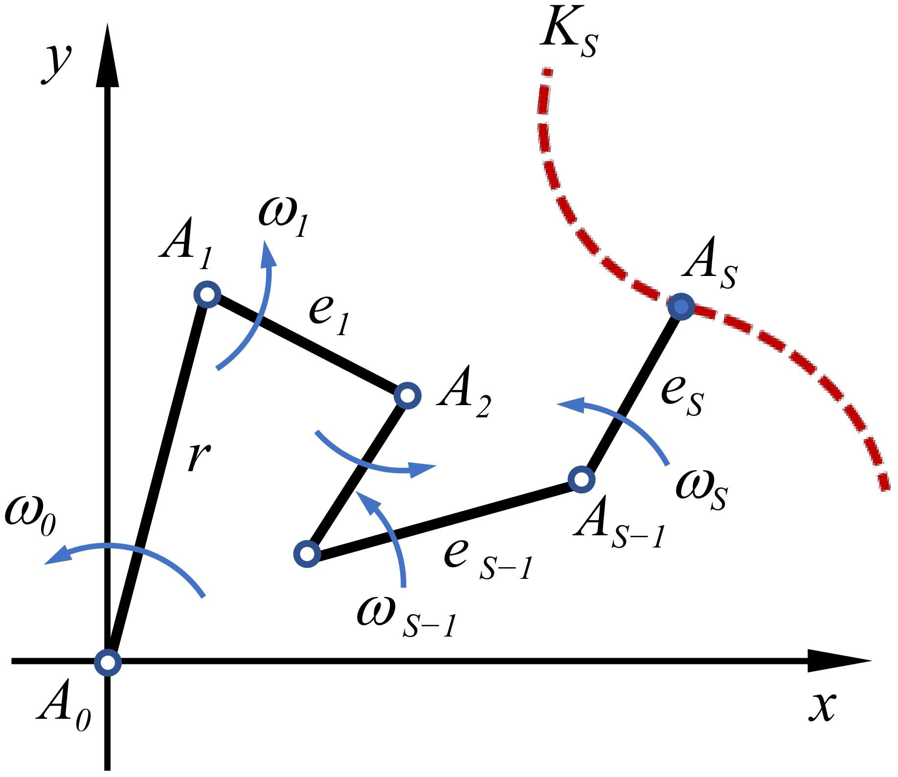
2. Geometry of Higher Trochoids
Higher trochoids were treated systematically for the first time by Wunderlich [
7] and are represented by complex functions. Thus, the two-parameter equations can be combined into one complex equation, reducing the mathematical effort. This approach was used in [
8] for a plane–curve representation. As shown in
Figure 1,
is defined by the planetary motion of several levers with corresponding angular velocities
. The position of the point
is determined by the sum of the vectors
and can be expressed as follows:
Here, e represents Euler’s number and
denotes an imaginary unit. The first radius
r is defined as the main radius and the levers
are used to describe the eccentricities of the profile. Point
is assumed to be the generating point. For simplicity,
has been replaced with
, yielding the following general form for higher trochoids:
If any e-lever shown in
Figure 1 rotates on its own plane, an arbitrary point on the corresponding plane can be selected as the pivot point for the next plane. The ‘extended’ or ‘shortened’ higher trochoidal curves can be generated using Equation (2), depending on the distance between a selected point and its pivot point. Closed curves with periodic symmetry are typically useful for technical applications. However, the ratios of the angular velocities
are not freely selectable for such curves.
Higher trochoidal curves are classified into the following three families ([
9]):
Equation (2) leads to the following relationship:
Equation (3) describes the higher epitrochoids of the nth order.
- -
Higher hypotrochoids
Equation (2) leads to the following relationship:
Equation (4) describes the higher hypotrochoids of the nth order.
- -
Higher hybrid (mixed) trochoid
Equation (2) leads to the following relationship, which describes higher hybrid (mixed) trochoids:
This trochoid has an order of . In essence, Equation (5) is the sum of Equations (3) and (4), where the term is considered only once.
For all three classes of curves, n describes the periodicity of the trochoid; therefore, it also represents the number of sides of the profile whose boundary contour is described by the corresponding equation.
Hybrid trochoidal profiles were also presented in [
9], where two real parameter functions were used to describe the geometry. Using the above methodology, the contour geometry can be determined via a single ‘complex’ equation, simplifying the investigations of a profile’s geometric and mechanical properties. If the function
conformably maps the boundary of a unit circle to the profile contour, the complex formulation should facilitate the investigation of the mechanical stresses in the profiles [
6,
10]. In [
11,
12], such formulations were used to solve the torsion problem for prismatic profile shafts.
Special features of higher hybrid (M) profiles
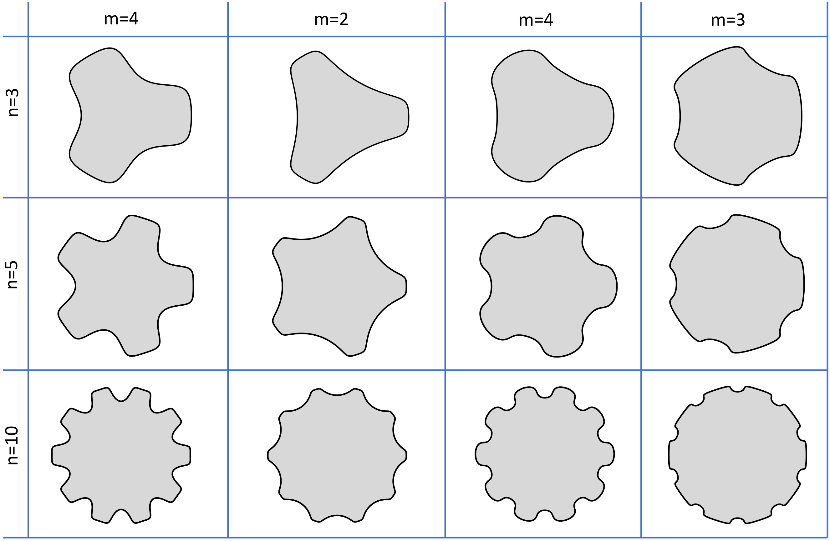
This study deals with the general description of hybrid (M) profiles based on Equation (5). By changing the periodicity n and the number of e values and their sign, innumerable profile contours can be obtained that can be adapted to any technical application.
Figure 2 presents examples of M-profiles, where m represents the order of the profile. A change in the
e values may produce concave, flat, or convex flanks while the general profile character remains unchanged.
3. Geometric Properties of M-Profiles
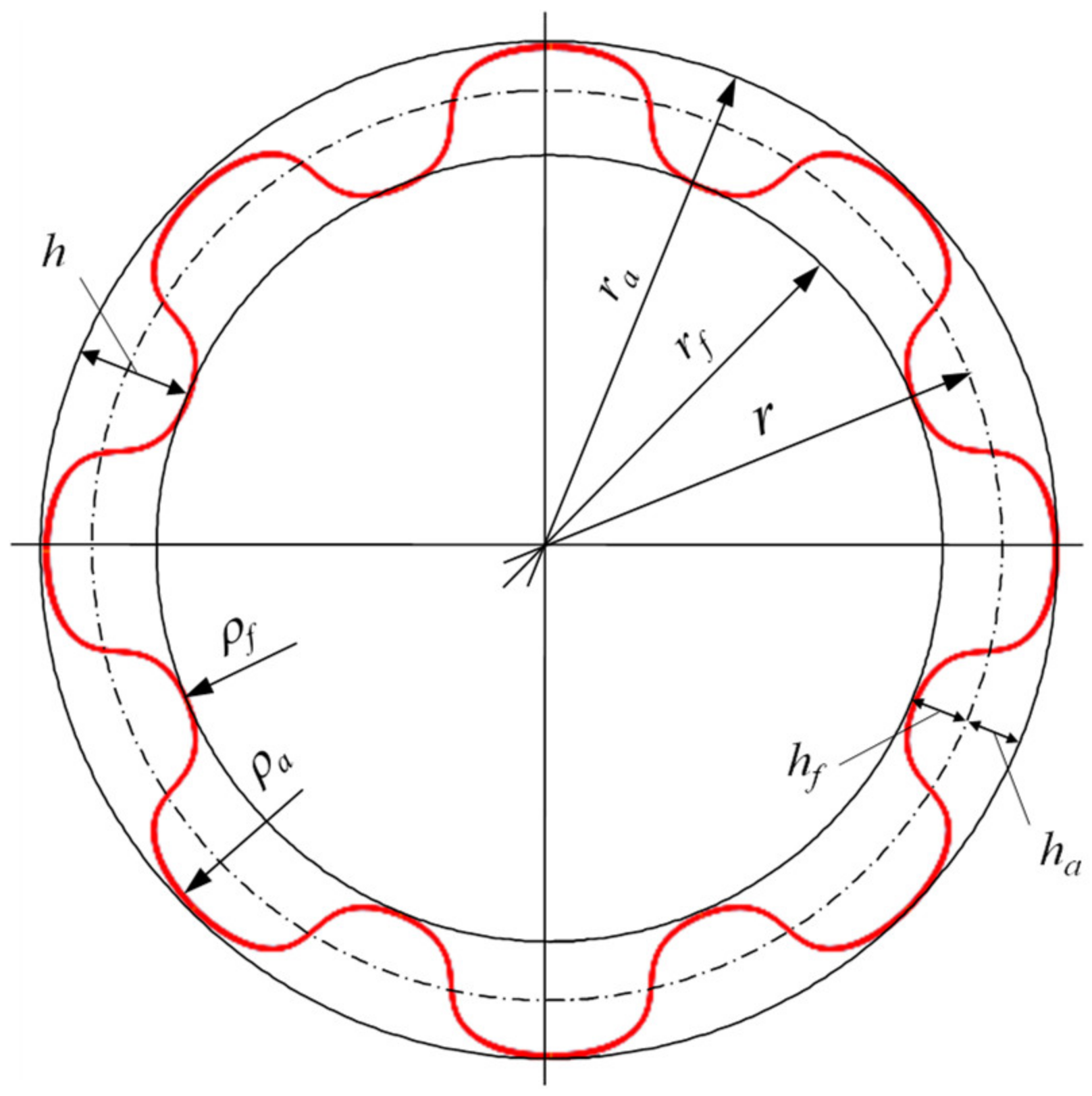
According to the contour based on Equation (5), the geometric properties of the profile, that is, the profile area, radii of the head circle (ra) and foot circle (rf), the contour curvatures, ρ, and the tooth height h can be determined. These variables determine the influences on the construction-space requirements and the profile form/friction-fit properties for application as a shaft–hub connection.
Figure 3 shows an example of the geometry sizes for an M-profile with eight teeth. The profile geometry can be changed depending on the eccentricities and adapted to predefined geometric conditions.
3.1. Area
The area enclosed by the contour
can be determined as follows [
8]:
where
Im[ ] indicates the imaginary part of the function, which is presented in square brackets.
3.2. Radii of Head Circle (ra) and Foot Circle (rf)
By substituting
into Equation (5), the following relationship is obtained:
Equation (7) describes the profile contour as a ‘complex’ function of the parameter angle
t. If
t = 0 is inserted into Equation (6), the radius of the head circle
is determined as follows:
that is,
The radius of the foot circle
can be determined by substituting
into Equation (7):
that is,
3.3. Tooth Height
Similar to the terminology of gear technology, the tooth height
h can be defined for M-profiles. It is defined as the sum of the addendum
and dedendum
, as follows (see also
Figure 3):
where
and
are applied.
3.4. Radius of Curvature
The radius of curvature can then be determined from the elementary differential geometry in complex form as follows [
8]:
The following relations hold for the functions
and
:
The radii of curvature at the contour head and foot areas ( and , respectively) are important for profile manufacturing and can be determined from Equation (10) with and , respectively.
4. M-Profiles with Four Eccentricities [1,2]
This effort aimed to combine the advantages of P3G profiles of DIN 32711 [
3] (low form/notch coefficient) with those of the splined shaft profiles of DIN 5486 [
4] (high form fit) in one profile. The M-profile contours were extensively investigated and optimised in [
1] with regard to torsional loading. To keep the scope of the investigations manageable, profile families are developed with four eccentricities while maintaining the adaptability of the contour to practical applications.
The following contour description applies to an M-profile with s = 2 (or 4 eccentricities):
Area
Accordingly, Equation (6) gives the following relationship for the area of the profile cross-section:
Head circle
In many practical applications, the head circle determines the installation space of the profile. The radius of the head circle can be determined from the contour equation (Equation (13)) for the contour head (at
t = 0) as follows:
Foot circle
As another characteristic, the foot-circle radius can be determined from Equation (13) with
, as follows:
Tooth height
The tooth height is calculated as the difference between the radius of the head circle and that of the foot circle:
The addendum and the dedendum are determined as follows:
As indicated by Equation (17), the tooth height depends only on and . According to Equations (18) and (19), the corresponding proportions and also depend on and .
Radius of curvature
The radii of curvature for the head and foot areas are determined using Equation (11) as follows:
plays an important role in selecting a suitable manufacturing method and can be adjusted by considering the eccentricity values in Equation (12). The concavity of the profile flank (and consequently the form-fit degree of the profile) can be determined using in Equation (21).
M-T04 Profiles
In [
1], the four simplified eccentricities
, and
were defined as functions of a basic or main eccentricity
to narrow the range of variants. The general form of Equation (13) was used as a basis, and extensive investigations were performed on the load-bearing capacities of profiles with a hub for torsional loading [
1,
13,
14]. The eccentricities
, and
are expressed as follows:
This results in the following contour description for the M-T04 profile family:
The corresponding parametric equations can be obtained as follows:
An analytical approach for resolving the torsion issue using conformal mappings was comprehensively presented in [
1].
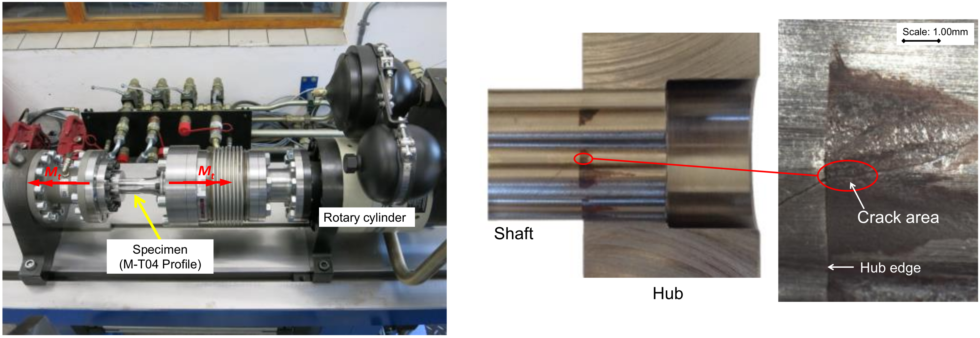
Figure 4 shows the testbench for the torsional load (left) and the cracking due to torsional loading (right) for the M-04-Profile studied in [
1].
Geometric properties of M-T04 profiles
From Equation (14), the area enclosed by the M-T04 contour can be easily derived for any number of sides
n, and the corresponding main eccentricity
:
Additionally, Equations (15) and (16) can be used to calculate the radii of the head and foot circles as follows:
The tooth height
h and its distribution can be determined from the parameter equations as functions of
n and
Additionally, the radii of the contour head and foot can be determined as follows:
5. Bending Stresses in Profiled Shaft
5.1. General Theory: Pure Bending
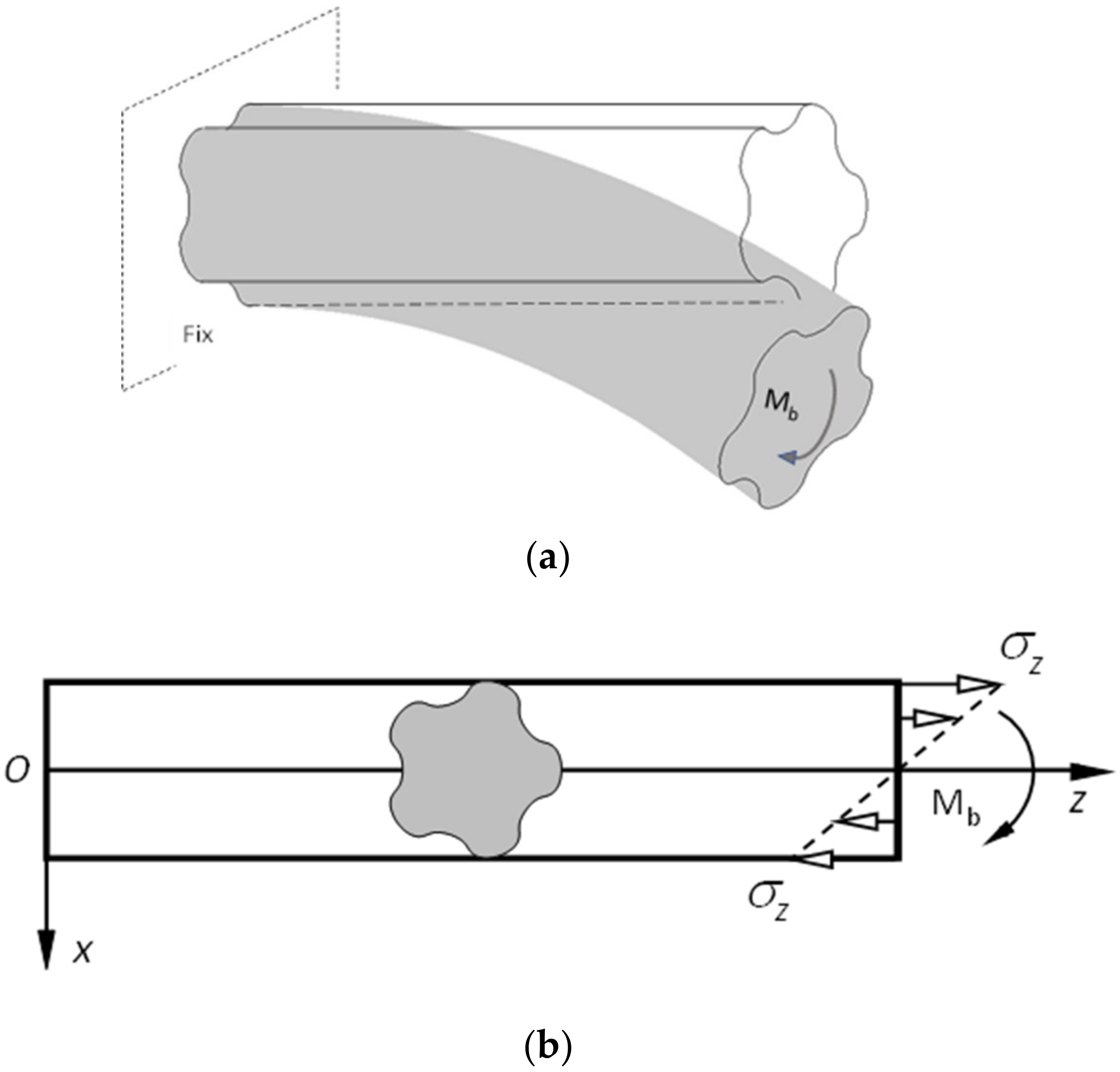
For prismatic beams with an arbitrary cross-section, the elementary approach can be used to solve for pure bending.
Figure 5a schematically represents a prismatic beam subjected to a bending load with a noncircular cross-section and five teeth.
Bending stress
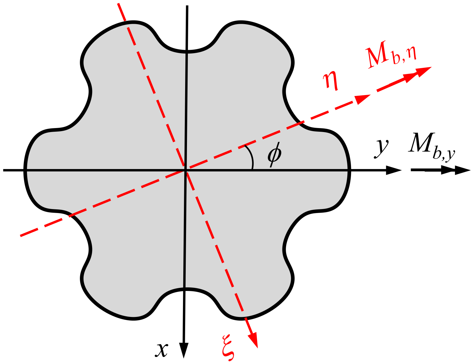
Figure 5b presents the coordinate system used to describe the stresses in this study. The
z-axis was set along the length of the shaft, and the
x-axis was set in the vertical direction. The shaft was fixed to the left. For convenience, the coordinate origin was placed at the centre of gravity of the left profile face. To solve this problem, the following elementary approach from the literature is used, where the equilibrium and compatibility conditions for the elastic bodies are satisfied [
6]:
It is assumed that the plane cross sections remain planar upon loading. The factor
in Equation (31) represents a constant value determined by the equilibrium of the bending stresses. The resulting moment of the stresses acting on the right side (or on any cross-section) remains in equilibrium with the bending load with respect to the
y-axis:
Substituting
from Equation (31) into (32) yields the following relationship, where
represents the moment of inertia of the profile section with respect to the
y-axis:
Therefore, the following relationship is valid:
Thus, the solution for the stresses can be obtained as follows:
Deflection
Displacements are determined using Hooke’s law and the corresponding relation between displacements and strain as follows [
6,
10]:
The deflection of the neutral axis is determined from
ux for
x =
y = 0, as follows:
Bending moment of inertia
Although the moments of inertia usually involve a double integral over the profile cross-section, this is reduced to a simple curvilinear integral over the profile contour using Green’s theorem, as follows [
10]:
The corresponding contour description based on Equation (13) is also advantageous. Cartesian coordinates can be easily obtained via elementary calculations using the complex functions, as follows (see [
15]):
By substituting Equation (38) into the definitions of the moments of inertia (Equation (37)), they are determined as follows, where
holds.
Equation (39) facilitates the determination of the moments of inertia when is available for the profile contour.
Rotational bending
Because a prismatic bar has technical applications as a rotating profile shaft, the bending moment of inertia should also be determined for rotated coordinates.
Figure 6 schematically represents an M-04 profile with six teeth in Cartesian coordinates.
The coordinates rotated by angles
are denoted as
and
. Owing to the tensorial property of moments of inertia, the following relationships are obtained for the rotated coordinate system using Mohr’s circle (see [
16]):
The moments of inertia remain invariant owing to the periodic symmetry of the cross-section of the M-contours presented in this paper based on Equation (13). Therefore, the following relationships are valid from Equation (39):
This property is advantageous when Equation (39) is used to determine the moments of inertia for the rotated cross-section. By substituting the values from Equation (38) into Equation (37) for an arbitrary rotation angle
, the following relationships are obtained:
The polar moment of inertia can be determined as follows:
5.2. General Solution for M-T04 Profiles
Moments of inertia
By substituting the eccentricities from Equation (23) into Equation (39), the following equations are obtained for the moments of inertia for any number of flanks
n and an arbitrary main eccentricity
e0:
Then, according to Equation (43), the following relationship for the polar moment of inertia is valid:
Therefore, the bending stress and deformations can be determined using Equations (35) and (36), respectively.
Bending stress
To obtain a general solution for the bending stress
based on (35), lever
x should be converted to the rotated coordinate system:
where
represents the rotation angle. If the values of
x and
y from Equation (24) are substituted into Equation (46), the following relationship is obtained for the rotated coordinate
on the profile contour (
):
The distribution of bending stress on the profile contour can be determined using the following equation:
By substituting from Equation (47) and from Equation (44) into Equation (48), the distribution of the bending stress on the profile contour can be determined.
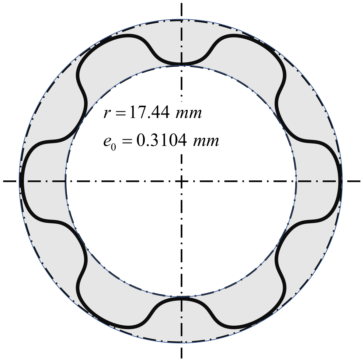
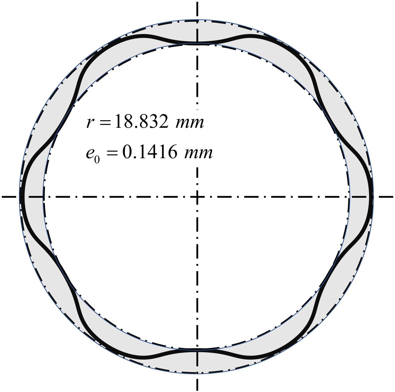
5.3. M-04 Profile from [1]
As an example, the profile experimentally investigated in [
1] for torsional loading (see
Figure 4) was used as a basis to investigate the bending behaviour. The corresponding geometric properties are
(
Figure 7). Equation (23) provides the following relationship for the contour of this profile:
The bending moment of inertia about the
x- or
y-axis of
with
is then calculated using (44). The solution of the bending stress for the profile contour (
) in the rotated coordinate system is obtained using (48) as follows:
with
By substituting Equation (52) into Equation (51), the following relationship can be obtained for the distribution of the bending stress on the lateral surface of the profiled shaft for an arbitrary rotation angle
:
In addition, numerical investigations were carried out using FEA to compare with Equation (52). The MSC-Marc programme system was used.
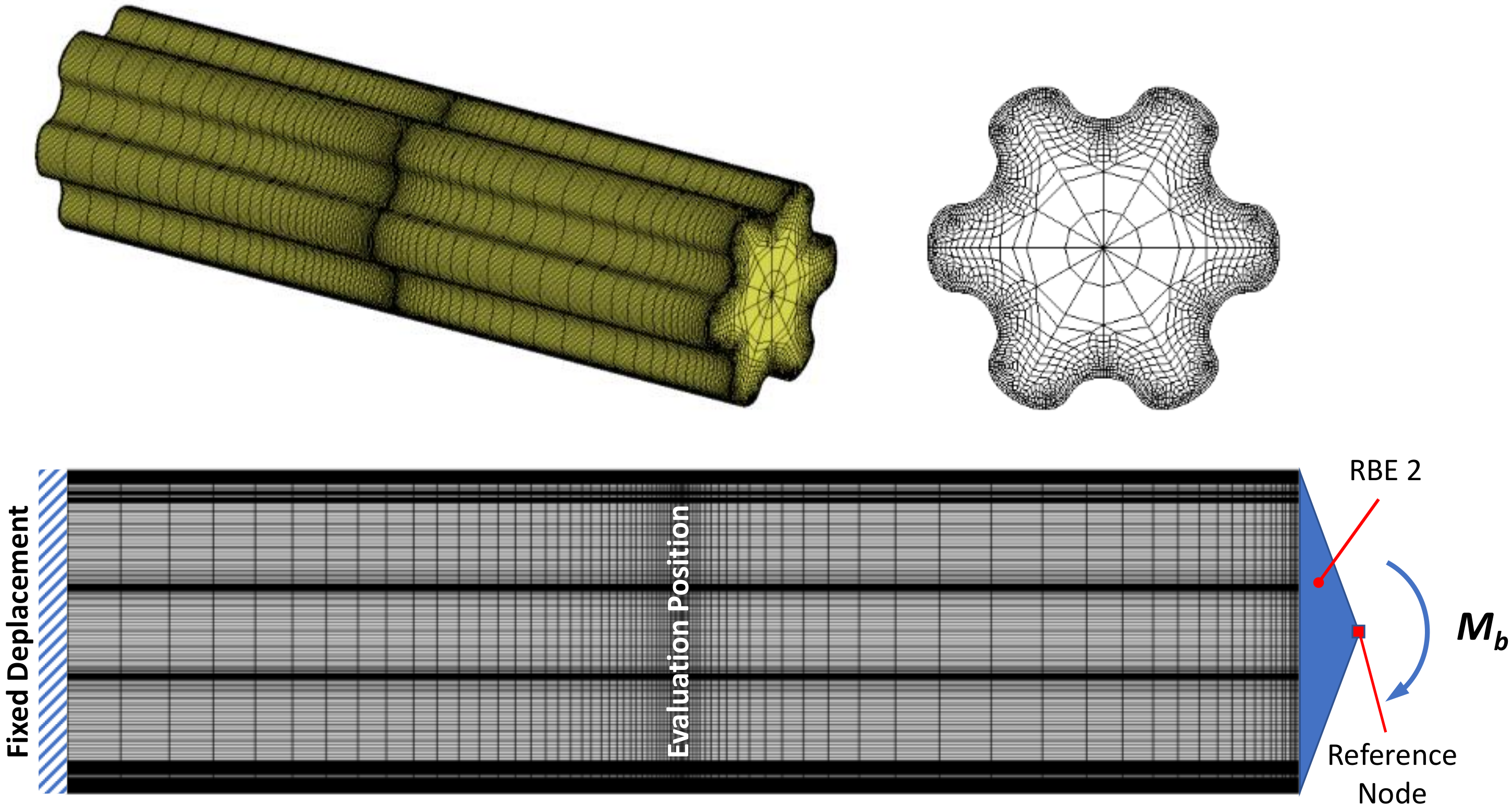
Figure 8 shows the mesh structure and the corresponding boundary conditions. The profiled shaft is fixed on the left side. The bending moment is transferred to the shaft’s right side via a reference node using REB2. The FE mesh contains 185,280 hexahedral elements with full integration (type 7 according to the Marc Element Library [
17]) and 202,258 nodes. The FE meshes were generated with the help of software written in Python language at the Chair of Machine Elements at the West Saxon University of Applied Sciences in Zwickau. The FE meshes were then transferred to the MSC-Marc program system and integrated into the pre-processing.
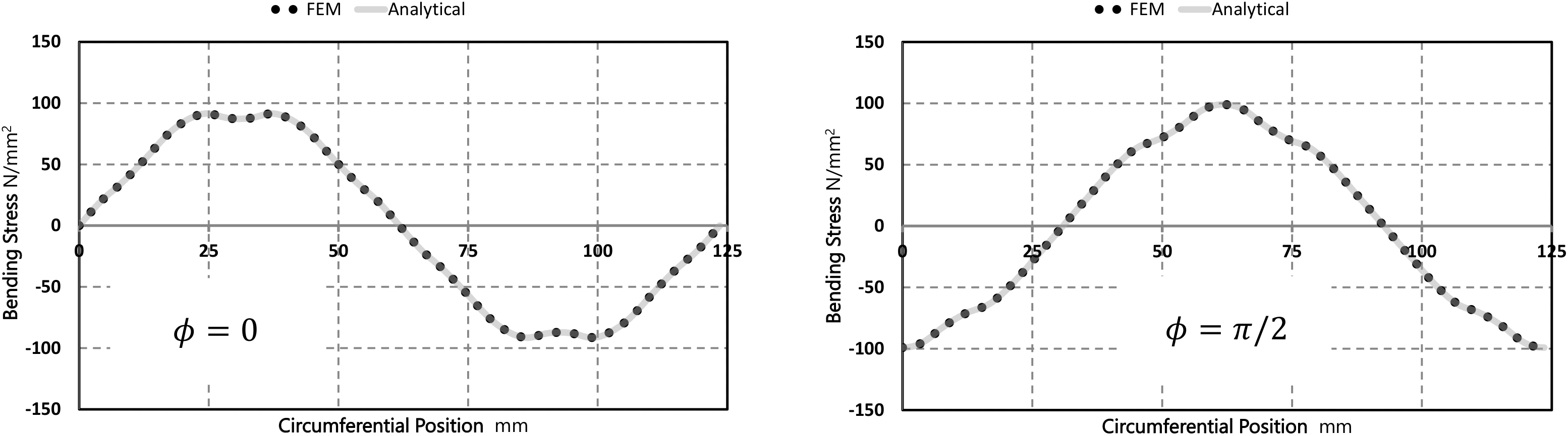
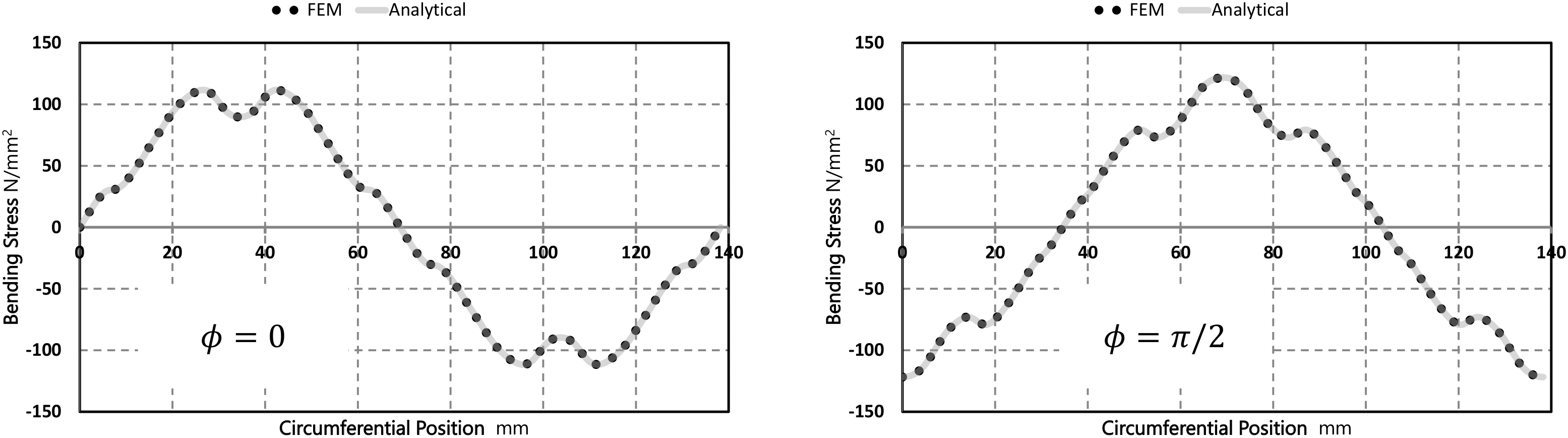
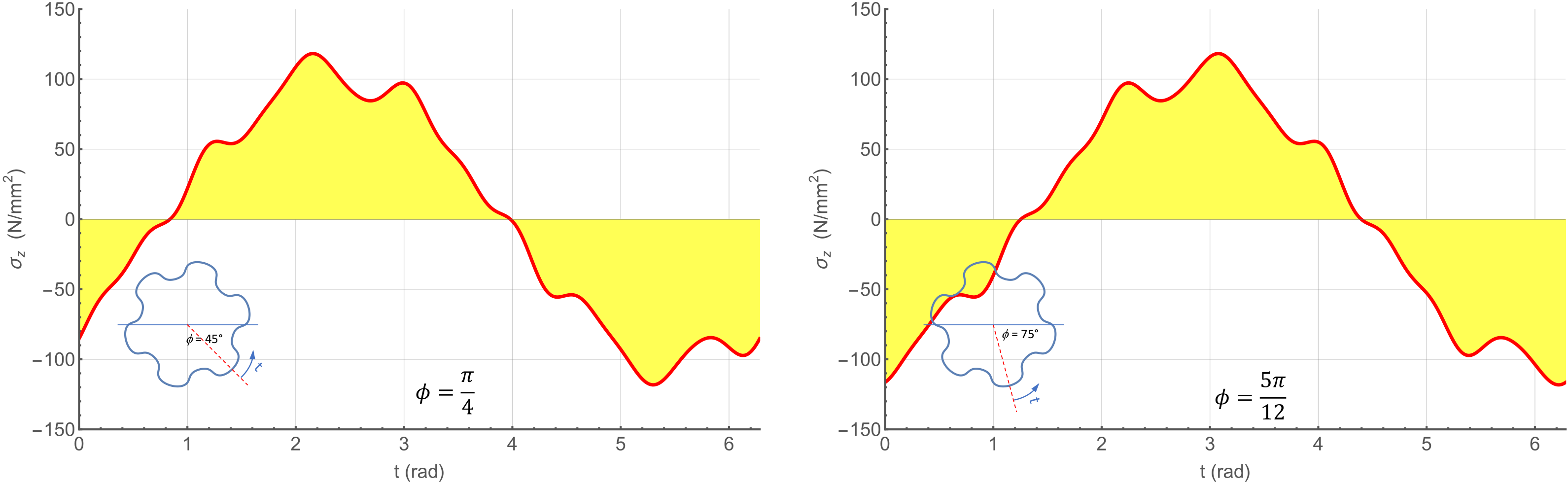
The stress distribution is determined for two angles of rotation (
and
) using Equation (52) and compared with the results of the finite-element (FE) analyses in
Figure 9, where
. As shown, the results agree well.
Figure 10 presents the bending stresses on the profile contour for different rotation angles, which were determined using Equation (52). As expected, the maximum stress occurred at
(or
) on the profile head.
5.4. Modified M-04 Profile Based on [2]
In another transfer project with industry [
2], the M-04 profile was modified for practical application as a shaft–hub connection in a transmission system. The geometric properties of the modified contour were
(
Figure 11).
According to Equation (23), the contour of this profile is expressed as follows:
From (44), the bending moment of inertia is determined as and .
The solution for the bending stress for the profile contour (
) in a rotated coordinate system is obtained using (48) as follows:
By substituting
from Equation (51) into Equation (54), the following relationship can be obtained for the distribution of the bending stress on the lateral surface of the profiled shaft for an arbitrary rotation angle
:
The distribution of the bending stress was determined for two angles of rotation (
and
) using Equation (55) and compared with the results of the FE analyses, as shown in
Figure 12, where
. Good agreement between the results was observed.
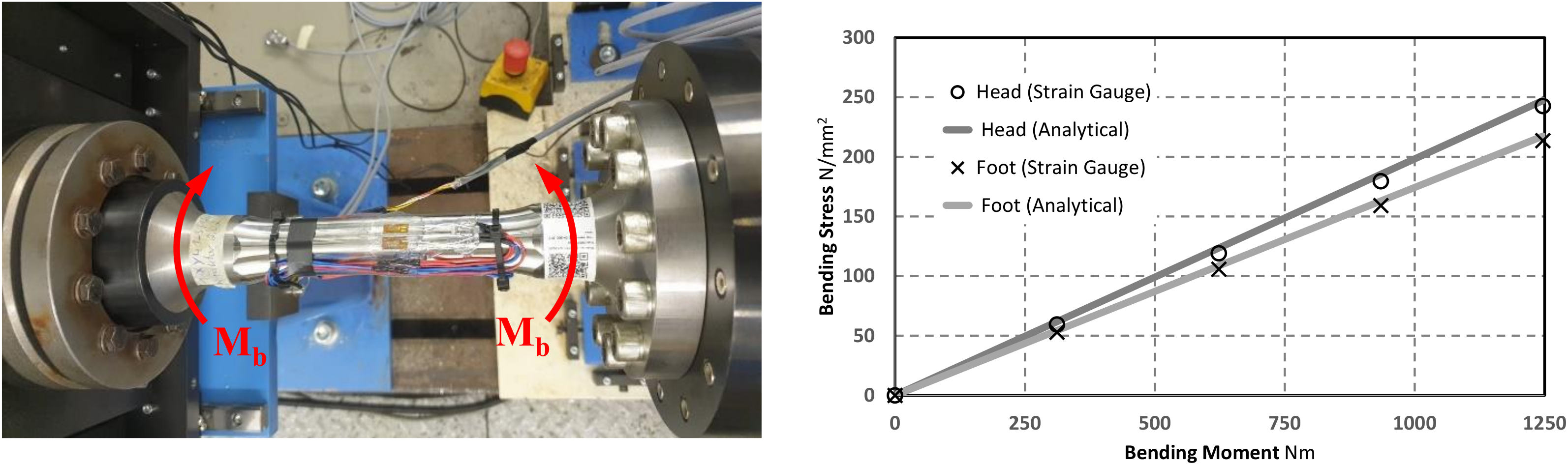
5.5. Experimental Investigations
In addition to analytical and numerical solutions, experimental measurements were performed using strain gauges (
Figure 13 left). A comparison of the experimental results with the solution obtained using Equation (36b) is presented in
Figure 13 right; as shown, good agreement was observed.
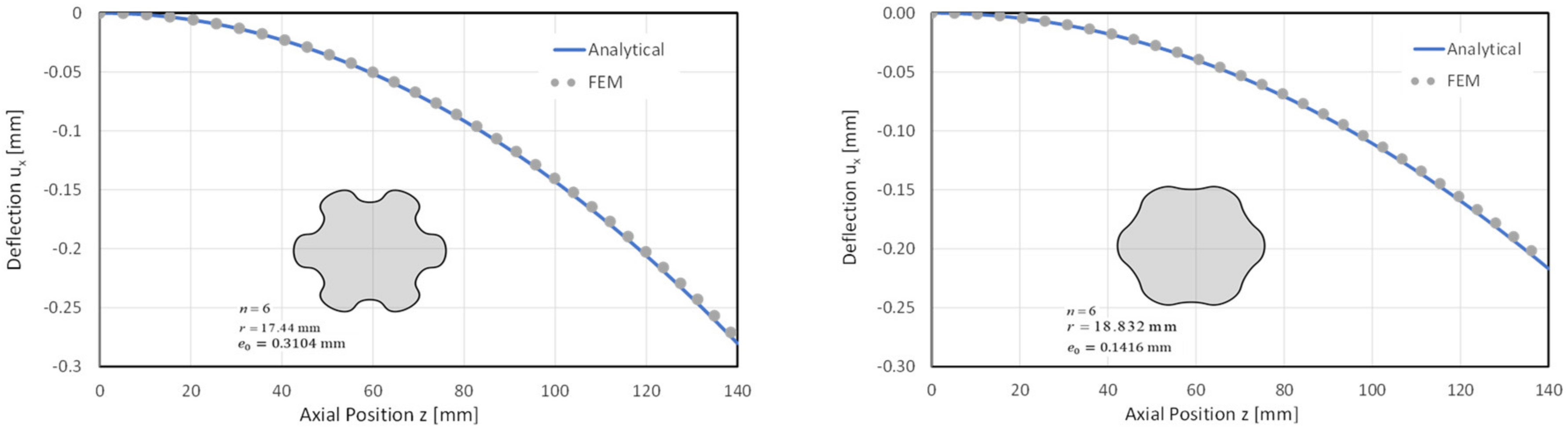
5.6. Deflection
The deflection can be easily determined from Equation (36a) as a function of the axial coordinate:
The shaft deflection was calculated for both M-04 [
1] and the modified profile [
2] for a length of
, with
and an elastic modulus of
for steel.
Figure 14 presents the deflection for both shaft profiles and a comparison with the numerical (FE analysis) results; as shown, good agreement was observed.
6. Conclusions
The geometric characteristics of the higher trochoids were systematically discussed in the first part of this paper. The advantages of such profiles, known as the M-T04 profile family, were represented for use as shaft–hub connections.
Because of a practical viewpoint, the geometrical features, such as head circle, root circle, tooth height, etc., were described analogously to the standardised tooth profiles for shaft-hub connections. In contrast to the standard tooth profiles, the higher trochoids have mathematically continuous contours.
The next part of the paper outlined a general theory of bending-loaded profile shafts. A general solution of the rotating bending stress and deformations for pure bending (without shear force) was presented. By properly formulating the geometric-mechanical relations of the trochoidal curves with the help of complex functions, closed solutions for the bending stresses and the elastic deformations in such profiles were derived. The obtained equations allow a quick design of the profiled shaft with the help of a simple pocket calculator without expensive FE analyses. The solution was directly applied to two M-04 profiles. The analytical results agreed very well with numerical and experimental findings.


