Stochastic Static Analysis of Planar Elastic Structures with Multiple Spatially Uncertain Material Parameters

Abstract

Engineering structures are often assembled from parts with different materials. When uncertainty quantification techniques are applied, the curse of dimensionality increases the computational complexity. Here, a stochastic Galerkin method for planar elasticity allowing for multiple regions with independent uncertain materials is introduced. The method allows for efficient solution of linear systems both in fully assembled and matrix-free formulations. The selection of the stochastic basis polynomials is performed using a priori knowledge of the decay of the random fields. The statistical quantities of interest are the expected solution and variance, both of which can be computed efficiently after the Galerkin system has been solved. Analysis of the results indicates that the proposed method is highly efficient in terms of both computational resource requirements and discretization of the stochastic dimensions. The results were verified with Monte Carlo and quasi-Monte Carlo methods.

1. Introduction

In engineering, structures made of multiple different materials are common. In this paper, the focus is on cases where the materials have uncertainties, that is, where they are random. The standard approach is to use an appropriate series representation such as Karhunen–Loève for inclusion of probabilistic variables (fields) into standard partial differential equations (PDEs). The resulting systems can then be solved either intrusively by designing specific solvers, or non-intrusively utilizing existing software frameworks.

Stochastic finite elements have a long history. The classic book by Ghanem and Spanos has been reprinted many times over the past decade [1]. Schenk and Shueller have interesting historical perspectives as well [2]. Following the seminal paper by Babuska et al. [3], where it was shown that the convergence rates are not restricted to those of Monte Carlo methods, there has been an explosion of publications in related topics. Uncertainties can occur in both materials and in loading and domain, which is to say, wherever manufacturing imperfections can arise in engineering. Numerical solution methods have been adjusted to handle the kind of systems that result from discretized stochastic PDEs. The Acta Numerica article by Schwab and Gittelson is an excellent overview [4], as is Xiu’s book [5]. Two relatively recent and accessible textbooks are those by Sullivan [6] and Soize [7].

Here, the focus is on a linear elasticity problem in which the computational domain is divided into subdomains, each with a random material parameter, namely, the Young’s modulus. The main modelling contribution of this paper is the following material model. It is assumed that each subdomain represents a manufactured part; therefore the correlations between different parts are ignored in the aggregate or global material model. The global material parameter is considered to be in tensor product form. Instead of trying to accommodate multiple random materials simultaneously, one could either try to homogenise [8] or alternatively to propagate uncertainties from different characteristic length scales to a final global scale [9,10]. The idea of representative volumes should be mentioned here as well [11].

There are many solution strategies for solving the resulting stochastic PDEs. These solution strategies can be broadly divided into intrusive and non-intrusive strategies. The main contribution to computational issues in this study lies in showing that the material model mentioned above can be effectively implemented within the standard stochastic Galerkin finite element method (sGFEM) framework, which is an intrusive approach. Currently, non-intrusive methods are used more widely. The main advantage of non-intrusive approaches is their ability to utilize the existing software infrastructure. The random input is evaluated at certain quadrature points and the underlying problem is then solved using those realizations of the input data. This collection of solutions can then be used to compute higher moments, such as variance, or to interpolate between the quadrature points. The gold standard is the Monte Carlo method and its many variations, including multi-level methods (see the much-cited work by Scheichl et al. [12]), and quasi-Monte Carlo, which has received a great deal of attention due to its theoretically better convergence properties (see the excellent work by Kuo and co-authors [13,14,15]). Collocation methods on sparse grids form another class of non-intrusive methods. Here, the Acta Numerica article by Bungartz and Griebel is the basic reference [16]. There has been much interest in fully adaptive schemes in collocation; see for example the recent paper by Lang et al. [17].

The deterministic part of the problem is discretized with the $hp$-version of the finite element method. This choice is motivated by the desire to minimize the number of degrees of freedom and prepare for future projects, such as those involving thin structures, where in order to avoid numerical locking the high-order methods are the preferred option. It is simultaneously both an advantage and disadvantage of sGFEM that one linear system has to be solved. In order to control the number of degrees of freedom, a priori selection of the stochastic basis polynomials is important. One heuristic approach originally proposed by Andreev [18] has been shown to perform remarkably well within this context. As planar elasticity leads to positive definite systems, conjugate gradients are a natural choice for iteration, provided that a suitable preconditioner can be constructed. Remarkably, a straightforward block-diagonal preconditioner can function extremely well. Furthermore, in the case of multiple random fields there exists an immediate matrix-free variant of the solution method. Similar problems have been considered by other authors as well, both from the point of view of preconditioning and of alternative formulations of the elasticity equations. Klawonn has considered the FETI domain-decomposition method in the $hp$-context [19], whereas recently Eigel and Gruhlke have successfully used FETI for the kind of problems discussed here [20]. Preconditioning of elasticity problems within the mixed FEM formulation has been discussed by Khan et al. in a very nice paper [21]. As already mentioned, the a priori selection of the basis polynomials is emphasised here. However, there exist adaptive schemes for simpler material models as well. In particular, the work of Bespalov is very interesting, as these methods can potentially be utilized in the $hp$-context [22].

The model configuration used here is shown in Figure 1. Using symmetry, the original 3D problem can be dimensionally reduced to a planar elasticity problem. In the numerical examples below, cases with either three (indicated with $(i,·)$, $i=1,2,3$) or eight materials are considered. Even though the problem setting is idealised, it is clear that similar configurations arise within the study of composite-type or sandwich-type structures, as well as multi-panelled designs such as pressure vessels. In the numerical experiments, it is assumed that while the expected value of the material parameter is constant, realizations of the material parameters may be discontinuous over regional boundaries. Problems with strong jumps between material parameters are an active area of research. A very interesting paper by Heinlein et al. discusses such problems within the kind of domain decomposition framework which may well be suitable in the context of this paper as well [23].

The rest of the paper is structured as follows. First, Navier’s elasticity equations are discussed, including the corresponding stochastic formulation. Next, the stochastic Galerkin method is reviewed in compact form along with definitions of all key elements needed. Readers who are familiar with the topics mentioned above can safely move directly to the description of the selection of the chaos polynomials and the tightly integrated iterative solver. The numerical experiments cover two configurations of random material fields, and a thorough analysis of the results is presented. Our conclusions are drawn in the final section.

2. Navier’s Equations of Elasticity

Here, Navier’s equations of elasticity are chosen to model the system of interest. One of the standard reference textbooks is Slaughter [24]. Let D be a domain representing a deformable medium subject to a body force $\mathbf{f}$ and a surface traction $\mathbf{g}$. The 2D model problem is then to find the displacement field $\mathbf{u}=(u_1,u_2)$ and the symmetric stress tensor $\sigma ={\left({\sigma }_{ij}\right)}_{i,j=1}^2$ such that

$$\begin{array}{ccc}\hfill \sigma & =\lambda div\left(\mathbf{u}\right)\mathbf{I}+2\mu ϵ\left(\mathbf{u}\right),\hfill & \hfill \mathrm{in}D\\ \hfill -div\left(\sigma \right)& =\mathbf{f},\hfill & \hfill \mathrm{in}D\\ \hfill \mathbf{u}& =\mathbf{0},\hfill & \hfill \mathrm{on}\partial D_D\\ \hfill \sigma ·\mathbf{n}& =\mathbf{g},\hfill & \hfill \mathrm{on}\partial D_N\end{array}$$

(1)

where $\partial D=\partial D_D\cup \partial D_N$ is a partitioned boundary of D. The Lamé constants are

$$\lambda =\frac{E\nu }{(1+\nu )(1-2\nu )},\mu =\frac{E}{2(1+\nu )},$$

(2)

with E and $\nu$ being Young’s modulus and Poisson’s ratio, respectively. Further, $\mathbf{I}$ is the identity tensor, $\mathbf{n}$ denotes the outward unit normal to $\partial D_N$, and the strain tensor is

$$ϵ\left(\mathbf{u}\right)=\frac{1}{2}(\nabla \mathbf{u}+\nabla {\mathbf{u}}^T).$$

(3)

The vector-valued tensor divergence is

$$div\left(\sigma \right)={\left(\sum _{j=1}^2\frac{\partial {\sigma }_{ij}}{\partial x_j}\right)}_{i=1}^2.$$

(4)

This formulation assumes a constitutive relation corresponding to linear isotropic elasticity with stresses and strains related by Hooke’s generalized law:

$${\sigma }_v=\left[\begin{array}{c}{\sigma }_{11}\\ {\sigma }_{22}\\ {\sigma }_{12}\end{array}\right]=\mathbf{D}(\lambda ,\mu )\left[\begin{array}{c}{ϵ}_{11}\\ {ϵ}_{22}\\ {ϵ}_{12}\end{array}\right]=\mathbf{D}(\lambda ,\mu ){ϵ}_v.$$

(5)

2.1. Weak Formulation

The weak formulation is defined in the standard manner. Begin with a function space $V_D=\{v:v\in H^1\left(D\right),v{|}_{\partial D_D}=0\}$ and state (Find $\mathbf{u}\in V_D\times V_D$) such that

$$a(\mathbf{u},\mathbf{v})=L\left(\mathbf{u}\right),\forall \mathbf{v}\in V_D\times V_D,$$

(6)

where the bilinear form

$$a(\mathbf{u},\mathbf{v})={\int }_D\sigma \left(\mathbf{u}\right):ϵ\left(\mathbf{v}\right)d\mathbf{x}$$

(7)

is the integrated tensor contraction

$$\sigma :ϵ=\sum _{i,j=1}^2{\sigma }_{ij}{ϵ}_{ij},$$

(8)

and $L\left(·\right)$ denotes the linear functional

$$L\left(\mathbf{v}\right)={(\mathbf{f},\mathbf{v})}_D+{(\mathbf{g},\mathbf{v})}_{\partial D_N}={\int }_D\mathbf{f}·\mathbf{v}d\mathbf{x}+{\int }_{\partial D_N}\mathbf{g}·\mathbf{v}d\mathbf{s}.$$

(9)

As usual, the kinematic relation and the constitutive matrix

$${ϵ}_v\left(\mathbf{u}\right)=\left[\begin{array}{cc}\frac{\partial }{\partial x_1}& 0\\ 0& \frac{\partial }{\partial x_2}\\ \frac{\partial }{\partial x_2}& \frac{\partial }{\partial x_1}\end{array}\right]\left[\begin{array}{c}{u}_1\\ u_2\end{array}\right],\mathbf{D}(\lambda ,\mu )=\left[\begin{array}{ccc}\lambda +2\mu & \lambda & 0\\ \lambda & \lambda +2\mu & 0\\ 0& 0& \mu \end{array}\right]$$

(10)

respectively, are specified for the purpose of rewriting the bilinear form as

$$a(\mathbf{u},\mathbf{v})={\int }_D{ϵ}_v{\left(\mathbf{u}\right)}^T\mathbf{D}(\lambda ,\mu ){ϵ}_v\left(\mathbf{v}\right)d\mathbf{x}.$$

(11)

2.2. Stochastic Formulation

A stochastic extension of Navier’s equations of elasticity follows by application of basic principles. Even though only the case of uncertain material parameters is considered in the experiments, the presentation here is for the full stochastic formulation. Letting $(\mathsf{\Omega },\mathsf{\Gamma },P)$ denote a probability space, where $\mathsf{\Omega }$ is a space of outcomes, $\mathsf{\Gamma }\subset 2^{\mathsf{\Omega }}$ is a sigma-algebra of events, and $P:\mathsf{\Omega }\to [0,1]$ is a probability measure on $\mathsf{\Omega }$, respectively, the uncertainties in the domain and material parameters of the physical problem are modelled assuming that there exists an explicit dependence of these quantities on the stochastic variable $\omega \in \mathsf{\Omega }$ via a priori known mappings $\omega \mapsto D^{\omega }$, $\omega \mapsto E^{\omega }$, $\omega \mapsto {\mathbf{f}}^{\omega }$ and that $\omega \mapsto {\mathbf{g}}^{\omega }$.

The stochastic problem can then be stated as follows: find the displacement field ${\mathbf{u}}^{\omega }:D^{\omega }\to {\mathbb{R}}^2$ and stress tensor ${\sigma }^{\omega }:D^{\omega }\to {\mathbb{R}}^{2\times 2}$ such that

$$\begin{array}{ccc}\hfill {\sigma }^{\omega }& ={\lambda }^{\omega }div\left({\mathbf{u}}^{\omega }\right)\mathbf{I}+2{\mu }^{\omega }ϵ\left({\mathbf{u}}^{\omega }\right),\hfill & \hfill \mathrm{in}{D}^{\omega }\\ \hfill -div\left({\sigma }^{\omega }\right)& ={\mathbf{f}}^{\omega },\hfill & \hfill \mathrm{in}{D}^{\omega }\\ \hfill {\mathbf{u}}^{\omega }& =\mathbf{0},\hfill & \hfill \mathrm{on}\partial D_{D^{\omega }}\\ \hfill {\sigma }^{\omega }·\mathbf{n}& ={\mathbf{g}}^{\omega },\hfill & \hfill \mathrm{on}\partial D_N^{\omega }\end{array}$$

(12)

where for P-almost every $\omega \in \mathsf{\Omega }$. Here, the stochastic dependence $\omega \mapsto E^{\omega }$ is propagated into the Lamé constants ${\lambda }^{\omega }$ and ${\mu }^{\omega }$ via Equation (2).

Analogously to the deterministic case, the stochastic system (12) can be expressed in weak form. Stochastic extensions for forms (7) and (9) can be defined by setting

$$a(\omega ;\mathbf{u},\mathbf{v})={\int }_{D^{\omega }}{\sigma }^{\omega }\left(\mathbf{u}\right):ϵ\left(\mathbf{v}\right)d\mathbf{x}$$

(13)

and

$$L(\omega ;\mathbf{v})={({\mathbf{f}}^{\omega },\mathbf{v})}_{D^{\omega }}+{({\mathbf{g}}^{\omega },\mathbf{v})}_{\partial D_N^{\omega }}.$$

(14)

The weak form of the stochastic problem then reads as follows: find ${\mathbf{u}}^{\omega }\in V_{D^{\omega }}\times V_{D^{\omega }}$ such that

$$a(\omega ;{\mathbf{u}}^{\omega },\mathbf{v})=L(\omega ;{\mathbf{u}}^{\omega })\forall \mathbf{v}\in V_{D^{\omega }}\times V_{D^{\omega }}$$

(15)

where for P-almost every $\omega \in \mathsf{\Omega }$.

3. Galerkin Method

The system’s stochastic dependence arises from the random material parameter, that is, from the Young’s modulus, $E^{\omega }$. The Karhunen–Loève expansion is used to express this random field with respect to a countable set of random variables and spatial shape functions. Another possibility would be to first choose a suitable spatial basis and then estimate the corresponding polynomial chaos coefficients from available data; see [25,26].

3.1. Deterministic Part: hp-Version

The finite element method (FEM) is the standard numerical method for solving elliptic partial differential equations. Because FEM is an energy minimization method it is eminently suitable for linear elasticity problems. The $hp$-FEM variant is the most efficient one [27,28]. With proper geometric grading of the meshes (see Figure 2a) and uniform polynomial order, exponential convergence can be achieved even in problems with strong corner singularities.

The idea behind the p-version is to associate degrees of freedom with topological entities of the mesh, in contrast to the classical h-version, where the association is with mesh nodes only. When both strategies are combined, the result is the $hp$-version. The shape functions are based on suitable polynomials, which are integrated Legendre polynomials here, and their supports reflect the related topological entity—nodes, edges, and the interior of the elements. The nodal shape functions induce a partition of unity. Moreover, due to the construction of shape functions, it is natural to have large elements in the mesh without any significant increase in the discretization error. The number of elements can be kept relatively low, as additional refinement can always be added via the elementwise polynomial degrees.

3.2. Probability Preliminaries

Let $(\mathsf{\Omega },\mathcal{F},P)$ be a probability space, $\mathsf{\Omega }$ the set of outcomes, $\mathcal{F}$ a $\sigma$-algebra of events, and P a probability measure defined on $\mathsf{\Omega }$. The space of square integrable random variables on $\mathsf{\Omega }$ is denoted by $L_P^2\left(\mathsf{\Omega }\right)$. Furthermore, for a Hilbert space $\mathcal{H}$, the related Bochner space is defined as

$$L_P^2(\mathsf{\Omega };\mathcal{H}):=\left\{u:\mathsf{\Omega }\to \mathcal{H}|{\int }_{\mathsf{\Omega }}{\left|\right|u\left(\omega \right)\left|\right|}_{\mathcal{H}}^{2}dP\left(\omega \right)<\infty \right\}.$$

(16)

In the case that $\mathcal{H}$ is a separable Hilbert space, this admits the decomposition $L_P^2(\mathsf{\Omega };\mathcal{H})\simeq L_P^2\left(\mathsf{\Omega }\right)\otimes \mathcal{H}$.

A standard approach is to transform a problem such as (15) into a parametric deterministic form by first assuming the family ${\left\{y_m\right\}}_{m\ge 1}:\mathsf{\Omega }\to \mathbb{R}$ to be mutually independent with ranges ${\mathsf{\Gamma }}_m$ and associating each $y_m$ with a complete probability space $({\mathsf{\Omega }}_m,{\mathsf{\Sigma }}_m,P_m)$, where the probability measure $P_m$ admits a probability density function ${\rho }_m:{\mathsf{\Gamma }}_m\to [0,\infty )$ such that

$$\mathrm{d}{P}_m\left(\omega \right)={\rho }_m\left(y_m\right)\mathrm{d}{y}_m,y_m\in {\mathsf{\Gamma }}_m$$

(17)

and the $\sigma$-algebra ${\mathsf{\Sigma }}_m$ is assumed to be a subset of the Borel sets of ${\mathsf{\Gamma }}_m$. Finally, it is assumed that the stochastic input data are finite.

For every application of the stochastic Galerkin method, a basis is needed for the space $L_P^2\left(\mathsf{\Omega }\right)$. The generalised polynomial chaos is introduced for this purpose. This provides a basis consisting of orthogonal polynomials of the input random variables. Orthogonal polynomials for various probability distributions can be constructed, and the use of these as the basis has been observed to yield optimal rates of convergence [29,30].

3.3. Karhunen–Loève Expansion

The idea behind Karhunen–Loève expansion is to represent the underlying random field as a linear combination of the eigenfunctions of the associated covariance operator. The distinguishing feature of Karhunen–Loève expansion compared to other linear expansions is that it minimizes the mean square truncation error [1].

Rewriting the random field $E^{\omega }$ with respect to a basis defined by the eigenfunctions of the covariance operator, the following Karhunen–Loève expansion is obtained:

$$E^{\omega }=E(\omega ,\mathbf{x})=E_0\left(\mathbf{x}\right)+\sum _{m=1}^{\infty }\sqrt{{\mu }_m}{\psi }_m\left(\mathbf{x}\right){\varphi }_m\left(\omega \right),$$

(18)

where $E_0\left(\mathbf{x}\right)$ denotes the expected value of the Young’s modulus. Moreover, the coefficients ${\mu }_m$ and the stochastic fluctuations ${\psi }_m\left(\mathbf{x}\right)$ are the eigenvalues and vectors of the underlying covariance function. The sequence ${\overline{\mu }}_m=\sqrt{{\mu }_m}$, $m=1,\dots$ is assumed to have a decay rate $\zeta$.

The random variables ${\left\{{\varphi }_m\right\}}_{m=1}^{\infty }$ are centered and orthogonal, however, they are not necessarily independent. Solutions to this issue include the Rosenblatt transformation [31] and introducing suitable auxiliary probability density functions, as suggested in [3]. In the numerical experiments below it is assumed that the random field $E(\omega ,\mathbf{x})$ is expressed with respect to a set of mutually independent uniformly distributed random variables.

Bounds for the decay of the eigenvalues and eigenfunctions of the Karhunen–Loève expansion are provided in [32].

3.4. Legendre Chaos

The aim here is to express the solution to our problem in a basis of orthogonal polynomials of the input random variables. Therefore, the choice of these basis polynomials depends on the probability distribution of the random variables appearing in the spectral expansion (18). Here, only uniformly distributed random variables are considered, leading to the choice of tensorised Legendre polynomials.

Let $\mathbf{y}=(y_1,y_2,\dots )$ be a vector of mutually independent random variables with a constant probability density. After possible rescaling of each of the random variables, ${\left\{y_m\right\}}_{m=1}^{\infty }$ is uniformly distributed in the interval $[-1,1]$. The stochastic space is then $\mathsf{\Gamma }={[-1,1]}^{\infty }$ with the underlying uniform product probability measure $\nu$. The expected value or mean of a random variable v is thus provided by $\mathbb{E}\left[v\right]={\int }_{\mathsf{\Gamma }}v\left(\mathbf{y}\right)d\nu \left(\mathbf{y}\right)$, and the variance is $\mathrm{Var}\left[v\right]=\mathbb{E}[{(v-\mathbb{E}\left[v\right])}^2].$ The set ${\left({\mathbb{N}}_0^{\infty }\right)}_c$ is the set of all multi-indices with finite support, i.e., ${\left({\mathbb{N}}_0^{\infty }\right)}_c:=\{\alpha \in {\mathbb{N}}_0^{\infty }|\#\mathrm{supp}\left(\alpha \right)<\infty \},$ where $\mathrm{supp}\left(\alpha \right)=\{m\in \mathbb{N}|{\alpha }_m\ne 0\}$; moreover, $\left|\alpha \right|={\sum }_{m\in \mathrm{supp}\left(\alpha \right)}\left|{\alpha }_m\right|$.

Two concepts, multivariate polynomials and expansion coefficients, are central.

Definition 1

(Multivariate polynomial). Let $\alpha \in {\left({\mathbb{N}}_0^{\infty }\right)}_c$. The multivariate polynomial ${\mathsf{\Lambda }}_{\alpha }\left(\mathbf{y}\right)$, called the “chaos polynomial”, is defined as

$$\begin{array}{c}\hfill {\mathsf{\Lambda }}_{\alpha }\left(\mathbf{y}\right)=\prod _{m=1}^{\infty }{\varphi }_{{\alpha }_m}\left(y_m\right)=\prod _{m\in \mathrm{supp}\alpha }{\varphi }_{{\alpha }_m}\left(y_m\right)\end{array}$$

(19)

where ${\left\{{\varphi }_m\right\}}_{m\ge 0}$ is a suitably normalized (univariate) polynomial sequence with ${\varphi }_0\equiv 1$.

For any given multi-index $\alpha \in {\left({\mathbb{N}}_0^{\infty }\right)}_c$, there exists a corresponding multivariate Legendre polynomial ${\mathsf{\Lambda }}_{\alpha }\left(\mathbf{y}\right):={\prod }_{m\in \mathrm{supp}\alpha }{L}_{{\alpha }_m}\left({\mathbf{y}}_m\right),$ where $L_p\left(x\right)$ denotes the univariate Legendre polynomial of degree p. Normalization $\mathbb{E}\left[{\mathsf{\Lambda }}_{\alpha }^2\right]=1$ for all $\alpha \in {\left({\mathbb{N}}_0^{\infty }\right)}_c$ is assumed implicitly; in other words, the univariate Legendre polynomials are scaled to be orthonormal with respect to the inner product $\frac{1}{2}{(·,·)}_{L^2\left([-1,1]\right)}$.

The system $\left\{{\mathsf{\Lambda }}_{\alpha }\left(\mathbf{y}\right)\right|\alpha \in {\left({\mathbb{N}}_0^{\infty }\right)}_c\}$ forms an orthonormal basis of $L_{\nu }^2\left(\mathsf{\Gamma }\right)$ [30]. Therefore, any square integrable random variable v can be written in series form (the polynomial chaos expansion of the random variable v):

$$\begin{array}{c}\hfill v\left(\mathbf{y}\right)=\sum _{\alpha \in {\left({\mathbb{N}}_0^{\infty }\right)}_c}{v}_{\alpha }{\mathsf{\Lambda }}_{\alpha }\left(\mathbf{y}\right)\end{array}$$

(20)

with convergence in $L_{\nu }^2\left(\mathsf{\Gamma }\right)$.

Definition 2

(Legendre Coefficient). The Legendre coefficients (or expansion coefficients) are provided by

$$v_{\alpha }={\int }_{\mathsf{\Gamma }}v\left(\mathbf{y}\right){\mathsf{\Lambda }}_{\alpha }\left(\mathbf{y}\right)d\nu \left(\mathbf{y}\right)=\mathbb{E}\left[v{\mathsf{\Lambda }}_{\alpha }\right].$$

(21)

The Legendre coefficients are defined on the deterministic discretization, that is, the finite element mesh. Therefore, it follows that the individual coefficients can be analysed as any standard finite element solutions.

As the definition above is abstract, any practical application has to include a strategy for truncating the polynomial chaos. In the case of a single random variable, a surprisingly efficient strategy introduced by Andreev can be employed for a priori filtering of the chaos. For the case of multiple materials, for example, the tensor product of the individual filtered bases is used.

3.5. Discretized System

Using (11) with $\mathbf{D}(\lambda ,\mu )=E\overline{\mathbf{D}}(\lambda ,\mu )$ and the definitions above, the parametric deterministic weak formulation becomes

$$\begin{array}{cc}\hfill & {\int }_{\mathsf{\Gamma }}{\int }_{D}E(\mathbf{y},\mathbf{x}){ϵ}_v{\left(\mathbf{u}(\mathbf{y},\mathbf{x})\right)}^T\overline{\mathbf{D}}(\lambda ,\mu ){ϵ}_v\left(\mathbf{v}(\mathbf{y},\mathbf{x})\right)\rho \left(\mathbf{y}\right)\mathrm{d}\mathbf{x}\mathrm{d}\mathbf{y}=\hfill \\ \hfill & {\int }_{\mathsf{\Gamma }}{\int }_D\mathbf{f}\left(\mathbf{x}\right)\mathbf{v}(\mathbf{y},\mathbf{x})\rho \left(\mathbf{y}\right)\mathrm{d}\mathbf{x}\mathrm{d}\mathbf{y}+{\int }_{\mathsf{\Gamma }}{\int }_{\partial D_N}\mathbf{g}\left(\mathbf{x}\right)\mathbf{v}(\mathbf{y},\mathbf{x})\rho \left(\mathbf{y}\right)\mathrm{d}s\mathrm{d}\mathbf{y}\hfill \end{array}$$

(22)

for all $\mathbf{v}\in L_{\nu }(\mathsf{\Gamma },H_0^1\left(D\right)\times H_0^1\left(D\right))$, where $\mathbf{y}:=(y_1,y_2,\dots )\in \mathsf{\Gamma }:={\mathsf{\Gamma }}_1\times {\mathsf{\Gamma }}_2\times \dots$ and $\rho \left(\mathbf{y}\right)\mathrm{d}\mathbf{y}:={\prod }_{m\ge 1}{\rho }_m\left(y_m\right)\mathrm{d}{y}_m.$ The unique solvability of (22) follows from the Lax–Milgram lemma.

After discretization and truncation after $\tilde{M}$ terms, the weak formulation reduces to the following linear system of equations:

$$\begin{array}{c}\hfill \left(G_0\otimes A_0+\sum _{m=1}^{\tilde{M}}{G}_m\otimes A_m\right)\mathbf{u}=s_0\otimes f_0+s_0\otimes g_0,\end{array}$$

(23)

where

$$A_0=a(\mathbf{u},\mathbf{v}),A_m={\int }_D\sqrt{{\mu }_m}{\psi }_m\left(\mathbf{x}\right){ϵ}_v{\left(\mathbf{u}\right)}^T\overline{\mathbf{D}}(\lambda ,\mu ){ϵ}_v\left(\mathbf{v}\right)d\mathbf{x},m=1,\dots ,\tilde{M},$$

(24)

are standard finite element (FEM) matrices, $f_0$ and $g_0$ are standard load vectors corresponding to respective forces, ${\left\{G_m\right\}}_{m=0}^{\tilde{M}}$ are stochastic moment matrices, and $s_0$ is a stochastic load vector; see [32] for details.

The stochastic load vector is provided by

$$\begin{array}{c}\hfill {\left[s_0\right]}_{\alpha }:={\int }_{\mathsf{\Gamma }}{\mathsf{\Lambda }}_{\alpha }\left(\mathbf{y}\right)\rho \left(\mathbf{y}\right)\mathrm{d}\mathbf{y}\end{array}$$

(25)

and the elements of the stochastic moment matrices are

$$\begin{array}{cc}\hfill {\left[G_0\right]}_{\alpha ,\beta }& :={\int }_{\mathsf{\Gamma }}{\mathsf{\Lambda }}_{\alpha }\left(\mathbf{y}\right){\mathsf{\Lambda }}_{\beta }\left(\mathbf{y}\right)\rho \left(\mathbf{y}\right)\mathrm{d}\mathbf{y}\mathrm{and}\hfill \\ \hfill {\left[G_m\right]}_{\alpha ,\beta }& :={\int }_{\mathsf{\Gamma }}{y}_m{\mathsf{\Lambda }}_{\alpha }\left(\mathbf{y}\right){\mathsf{\Lambda }}_{\beta }\left(\mathbf{y}\right)\rho \left(\mathbf{y}\right)\mathrm{d}\mathbf{y},m=1,\dots ,\tilde{M},\hfill \end{array}$$

(26)

where $\alpha ,\beta \in \mathcal{A}\subset {\left({\mathbb{N}}_0^{\infty }\right)}_c$. It is known that the stochastic moment matrices ${\left\{G_m\right\}}_{m=1}^{\tilde{M}}$ exhibit a nontrivial sparsity pattern [32]; in addition, $G_0$ is a diagonal matrix.

3.6. Response Statistics

The calculation of statistical moments from the polynomial chaos representation is straightforward. Suppose that the polynomial chaos expansion of a random variable v is approximated by

$$v_{\mathcal{A}}\left(\xi \right)=\sum _{\alpha \in \mathcal{A}}{v}_{\alpha }{\mathsf{\Lambda }}_{\alpha }\left(\xi \right)$$

(27)

for some multi-index set $\mathcal{A}\subset {\left({\mathbb{N}}_0^{\infty }\right)}_c$.

$$\mathbb{E}\left[v_{\mathcal{A}}\right]=\mathbb{E}\left[\sum _{\alpha \in \mathcal{A}}{v}_{\alpha }{\mathsf{\Lambda }}_{\alpha }\right]=v_0$$

(28)

and the variance

$$\mathrm{Var}\left[v_{\mathcal{A}}\right]=\mathbb{E}\left[{\left(\left(\sum _{\alpha \in \mathcal{A}}{v}_{\alpha }{\mathsf{\Lambda }}_{\alpha }\right)-v_0\right)}^2\right]=\left(\sum _{\alpha \in \mathcal{A}}{v}_{\alpha }^2\right)-v_0^2.$$

(29)

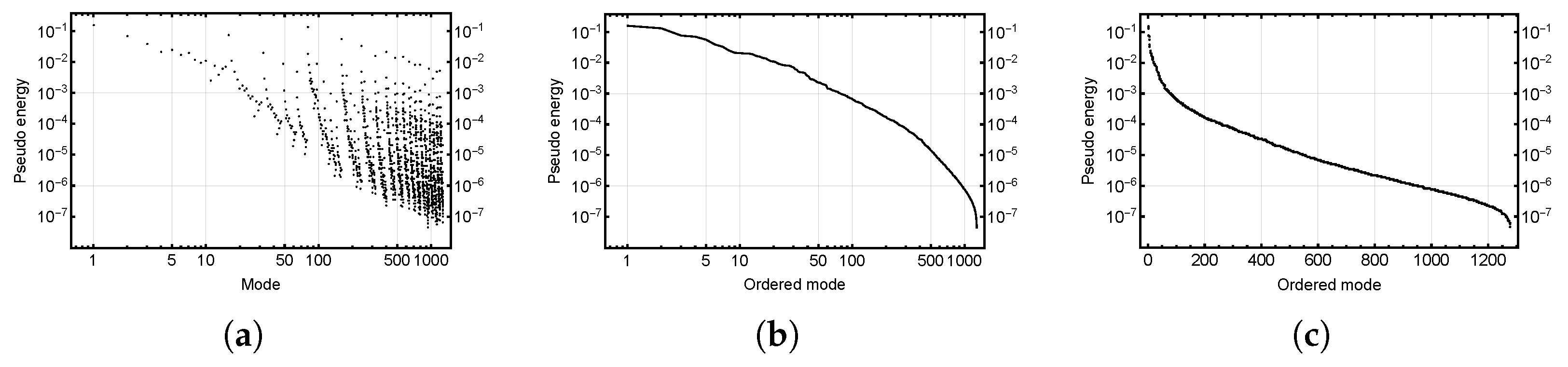
4. Selection of Chaos Polynomials

In the battle with the Curse of Dimensionality, it is necessary to select a truncation scheme for the polynomial chaos. Selecting the optimal index set a priori in the sGFEM setting remains an active research question; for foundations see, e.g., [18,33,34] and the references therein for more information.

4.1. Standard Truncation Schemes

Standard choices for the index set $\mathcal{A}$ are the isoTP and isoTD index sets.

Definition 3

(Isotropic tensor product index set). Let $N\in \mathbb{N}$ and $K\in {\mathbb{N}}_0$. The isoTP index set is provided by

$$\begin{array}{c}\hfill \mathtt{isoTP}(N,K)=\left\{\alpha \in {\left({\mathbb{N}}_0^{\infty }\right)}_c|\underset{n=1,\dots ,N}{max}{\alpha }_n\le K;{\alpha }_n=0,n>N\right\}.\end{array}$$

(30)

Definition 4

(Isotropic total degree index set). Let $N\in \mathbb{N}$ and $K\in {\mathbb{N}}_0$. The isoTD index set is defined as

$$\begin{array}{c}\hfill \mathtt{isoTD}(N,K)=\left\{\alpha \in {\left({\mathbb{N}}_0^{\infty }\right)}_c|\sum _{n=1}^N{\alpha }_n\le K;{\alpha }_n=0,n>N\right\}.\end{array}$$

(31)

The isotropic index sets are often preferred due to their ease of construction. However, the cardinalities of the isoTP and isoTD index sets are ${(K+1)}^N$ and $\left(\genfrac{}{}{0pt}{}{N+K}{K}\right)$, respectively, and hence the isotropic index sets grow rapidly when either N or K is increased. Therefore, as the isoTD index set grows slower than the isoTP index set, the isoTD index set is often preferred over the isoTP index set.

4.2. Andreev’s Selection Algorithm

In the context of Galerkin methods, Algorithm 1 originally by Andreev [18] has proven to be very efficient. The idea is to compute a priori weight estimates of the multi-indices satisfying a tolerance criterion.

The algorithm requires two auxiliary concepts. Let $c_0$ be the collection of strictly decreasing sequences of positive real numbers bounded above by one and tending to zero:

$$\begin{array}{c}\hfill c_0=\{\overline{\mu }=({\mu }_1,{\mu }_2,\dots )\in {\mathbb{R}}_{+}^{\mathbb{N}}|\underset{m\to \infty }{lim}{\mu }_m=0\mathrm{and}1>{\mu }_1\ge {\mu }_2\ge \dots \}.\end{array}$$

(32)

Furthermore, each multi-index $\alpha \in \mathcal{A}$ can be stored in the sparse format

$$\begin{array}{c}\hfill {\displaystyle \mathrm{SPARSE}}(\alpha ,{\overline{\mu }}^{\alpha })\equiv (\left\{(m,{\alpha }_m)\right|{\alpha }_m\ne 0\},{\overline{\mu }}^{\alpha })\end{array}$$

(33)

as a sorted set of pairs (ordered by the first component) and a real number.

Algorithm 1 Andreev’s Selection [18].

Given $\epsilon >0$, $\overline{\mu }\in c_0$, set ${\alpha }_0=(0,0,\dots )$. Compute $\mathcal{A}\leftarrow \left\{{\displaystyle \mathrm{SPARSE}}({\alpha }_0,1)\right\}\cup {\displaystyle \mathrm{ENUMERATE}}({\alpha }_0,1,1)$ Function ${\displaystyle \mathrm{ENUMERATE}}(\alpha ,m,{\epsilon }_{\alpha })$ with local variables α, m and ${\epsilon }_{\alpha }$ returns a set $\overline{\alpha }\subset \mathcal{A}$ – Let $\overline{\alpha }=\varnothing$ – emphIf ${\overline{\mu }}_m{\epsilon }_{\alpha }<\epsilon$ return $\overline{\alpha }$ – For $n=0,1,\dots$ * Set $\overline{\alpha }\leftarrow \overline{\alpha }\cup {\displaystyle \mathrm{ENUMERATE}}(\alpha ,m+1,{\epsilon }_{\alpha })$ * Set ${\alpha }_m\leftarrow {\alpha }_m+1$ and ${\epsilon }_{\alpha }\leftarrow {\overline{\mu }}_m{\epsilon }_{\alpha }$ * If ${\epsilon }_{\alpha }<\epsilon$ return $\overline{\alpha }$ * Set $\overline{\alpha }\leftarrow \overline{\alpha }\cup \left\{{\displaystyle \mathrm{SPARSE}}(\alpha ,{\epsilon }_{\alpha })\right\}$ Return$\mathcal{A}$

    The following examples illustrate how the selection is performed. The notation $L_a^b$ indicates a normalised Legendre polynomial with degree a in stochastic dimension b. Notice that in the first example, if the process is repeated with the given decay rate and lower tolerance, the first 16 polynomials would appear in the same order.

Example 1.

Let the decay rate $\zeta =2$ with coefficients ${\overline{\mu }}_m=1/{(m+1)}^{\zeta }$. Setting tolerance $\epsilon =1/100$, the selection algorithm produces a set

$${\mathsf{\Lambda }}_{\mathcal{A}}=\left\{1,L_1^1,L_1^2,L_1^3,L_2^1,L_1^4,L_1^5,L_1^1{L}_1^2,L_1^6,L_1^7,L_1^1{L}_1^3,L_3^1,L_1^8,L_2^2,L_1^9,L_1^1{L}_1^4\right\}.$$

(34)

The stochastic dimension is 9, $\left|\mathsf{\Lambda }\right|=16$.

Example 2.

Let the decay rate $\zeta =3$ with coefficients ${\overline{\mu }}_m=1/{(m+1)}^{\zeta }$. Setting tolerance $\epsilon =1/100$, the selection algorithm produces a set

$${\mathsf{\Lambda }}_{\mathcal{A}}=\left\{1,L_1^1,L_1^2,L_1^3,L_2^1\right\}.$$

(35)

The stochastic dimension is 3, $\left|\mathsf{\Lambda }\right|=5$.

The sum of all moment matrices ${\sum }_i{G}_i$ is

$$\left(\begin{array}{ccccc}1& \frac{1}{\sqrt{3}}& \frac{1}{\sqrt{3}}& \frac{1}{\sqrt{3}}& 0\\ \frac{1}{\sqrt{3}}& 1& 0& 0& \frac{2}{\sqrt{15}}\\ \frac{1}{\sqrt{3}}& 0& 1& 0& 0\\ \frac{1}{\sqrt{3}}& 0& 0& 1& 0\\ 0& \frac{2}{\sqrt{15}}& 0& 0& 1\end{array}\right).$$

(36)

The selection algorithm is performed independently on all random variables and the full basis is taken to be a Kronecker product of the individual bases. The corresponding stochastic moment matrices are simply Kronecker products of the individual ones, and naturally inherit their overall structure; of course, the products are much sparser. However, the matrix representation of the discretized system does not change. This is in fact the key reason why implementing the proposed model is relatively straightforward if an existing Galerkin solver is available.

5. Iterative Solver Formulation

The curse of dimensionality leads to large linear systems in the context discussed here. It is natural to consider iterative methods, and indeed the systems of type (23) lend themselves naturally to such methods. There are two inherent advantages: the action of the operator (matrix-vector multiply) can be written in a matrix-free fashion, and more importantly, the block-diagonal preconditioner of the form $P=I\otimes A_0$ is highly effective [35].

In practice, the implementation of the preconditioned conjugate gradients is straightforward. Although the linear systems (23) are inherently sparse, by judiciously folding and unfolding the temporary vectors and matrices, respectively, many computations can in fact be computed using full matrix–matrix or BLAS3 routines. One such implementation is outlined in Algorithms 2–4.

Algorithm 2 Preconditioner: $M\left(·\right)$.

Given Matrix $A_0$, vector b, Solve $A_{0}X=$ Folded column-wise b Return X

Algorithm 3 Matrix-Vector Multiply: $A\left(·\right)$.

Given matrices $A_i$, $G_i$, $i=1,\dots$, and vector x. $G_0$ is assumed to be an identity matrix. $U:=$Folded column-wise x $V:=A_{0}U+{\sum }_i{G}_i{U}^T{A}_i^T$ Return V

Algorithm 4 Conjugate Gradient Method [36].

Given matrix-vector multiply: $A\left(·\right)$, and preconditioner: $M\left(·\right)$. Compute $r_0:=b-A\left(x_0\right),z_0:=M\left(r_0\right),p_0:=z_0,$ For $j=0,1,\dots ,$ until convergence – ${\alpha }_j:=(r_j,r_j)/(A\left(p_j\right),p_j)$ – $x_{j+1}:=x_j+{\alpha }_j{p}_j$ – $r_{j+1}:=r_j-{\alpha }_{j}A\left(p_j\right)$ – $z_{j+1}:=M\left(r_{j+1}\right)$ – ${\beta }_j:=(z_{j+1},r_{j+1})/(z_j,r_j)$ – $p_{j+1}:=z_{j+1}+{\beta }_j{p}_j$ Return x

In the preconditioner one could opt for full factorization of the $A_0$, since the efficiency gains are derived from repeated solves of the same system with multiple right-hand-sides.

In the matrix-vector multiply, the action of the matrix $G_i$ can be broken down to a sequence of Kronecker products if there are multiple random fields involved. Technically, the index i can be taken as a multi-index indicating the respective mass matrices participating in the action. Similarly, the matrices $A_i$ could be integrated on demand rather than prior to the start of the solution process. Deciding on the proper course of action depends on the available computational resources and time constraints, of course.

As is well known, Krylov methods cannot be reliably accelerated using initial solutions. However, selection of a proper convergence criterion can always be considered. For systems with millions of degrees of freedom, the tolerance in the norm of the residual has to be chosen carefully. In fact, it might be more meaningful to use a physical quantity of interest such as convergence in the energy of the expected solution or the variance of the components.

6. Numerical Experiments

In the numerical experiments, two configurations are considered: (a) three regions and (b) eight regions. The regions are indicated in Figure 1 above. In all cases, the covariance functions are implicit; in other words, the KL-expansions are synthetic with the easier analysis and reproducibility of the results in mind. The expected value of the random variable parameter, the Young’s modulus, is constant in all regions. This choice was made to focus on the variance. In a more realistic scenario, there would be jumps in the expected values as well, although then the effect of the uncertainty would be more difficult to quantify precisely.

The material constants adopted for all simulations were as follows: $E_0=2.069\times {10}^{11}$ $\mathrm{MPa}$, $\nu =1/3$. The actual value of $E_0$ is superfluous, as everything has been scaled in order for the effective Young’s modulus to be $E^{\omega }=E(\omega ,\mathbf{x})=E_0\left(\mathbf{x}\right)(1+{\sum }_{m=1}^{\infty }{\overline{\mu }}_m{\psi }_m\left(\mathbf{x}\right){\varphi }_m\left(\omega \right)),$ and hence everything is computed as if $E_0\left(\mathbf{x}\right)=1$. As all reported results are relative in nature, this convenience choice does not affect our conclusions in any way. The stochastic fluctuations are defined for the indexed regions simply as ${\psi }_m(x,y)=cos\left(mx\right)$ for odd layers or regions and ${\psi }_m(x,y)=sin\left(my\right)$ for even layers or regions, where the coordinates $(x,y)$ are used instead of $(x_1,x_2)$. As in Examples 1 and 2 for the decay rate $\zeta$, the coefficients are taken to be ${\overline{\mu }}_m=1/{(m+1)}^{\zeta }$. The loading is a unit traction $\mathbf{g}$ action on one section of the boundary (see Figure 1), and there is no body force, that is, $\mathbf{f}=0$.

In both configurations, the deterministic part of the computational domain and its discretization is kept constant; the geometrically graded mesh is shown in Figure 2a. The polynomial order is constant $p=4$. In both cases, the loading is unit traction force acting on $u_2$ along the horizontal segment at $y=4/3$.

In the analysis of the results, two aspects of the method are highlighted: visualization of the higher moments (variance) and indirect quality assessment of the chosen stochastic basis. The latter is based on convergence analysis of the Legendre coefficients in various norms. Note that no attempt to conduct a convergence study with balanced errors in the deterministic and stochastic parts is made; the focus is solely on the a priori selection of the basis.

As the linear systems become very large, it is of interest to assess the efficiency of the selected basis polynomials. Given the tensor construction, the basis polynomials can be ranked by the properties of their Legendre coefficients. Three norms or norm-like quantities of interest are considered here: $L^2$-norm, $H_0^1$-seminorm, and “pseudoenergy” ${\parallel ·\parallel }_{A_0}$, where ${\parallel u\parallel }_{A_0}=\sqrt{u^T{A}_{0}u}$. The norms are computed component-wise, whereas the pseudoenergy is taken for the whole Legendre coefficient.

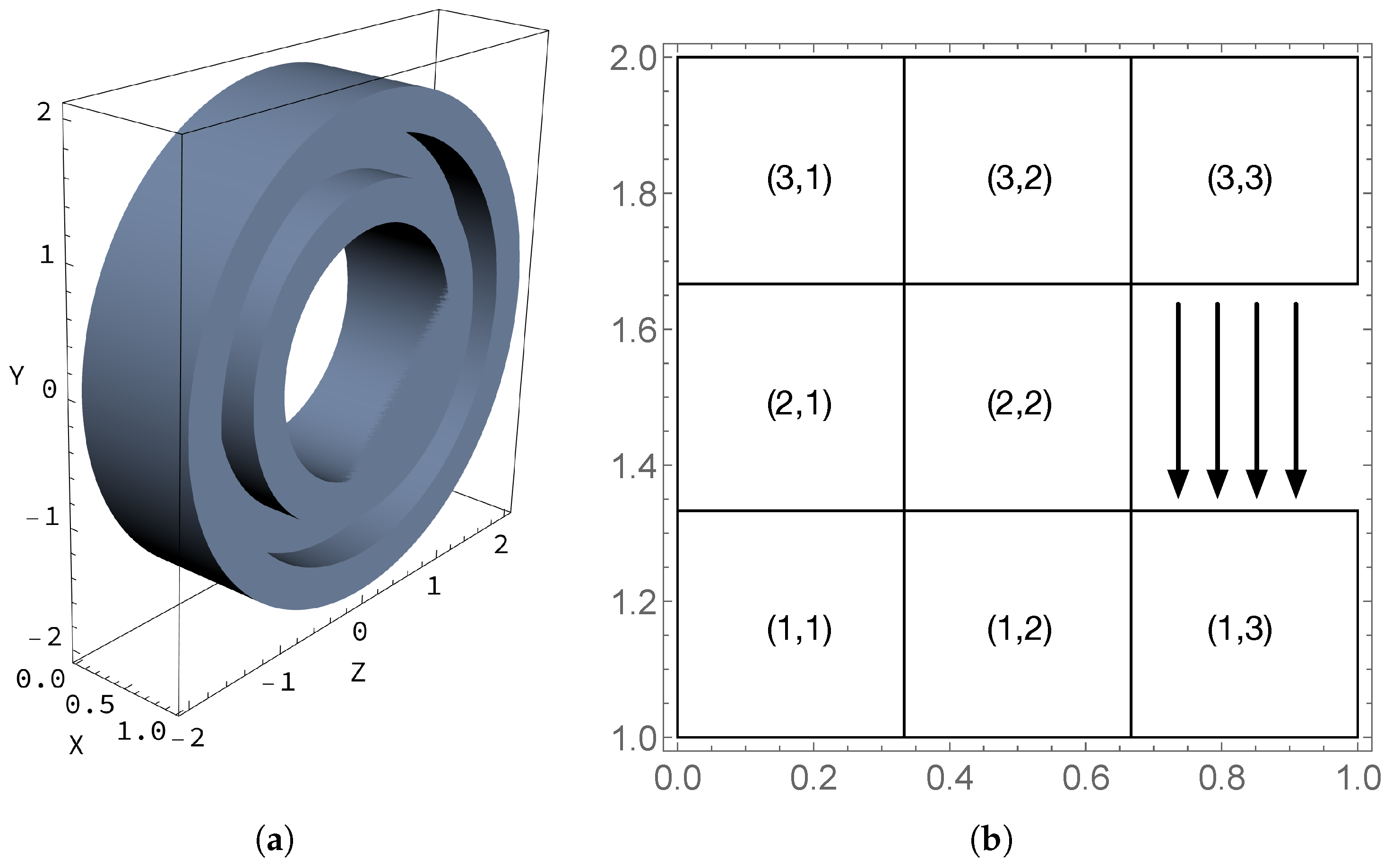
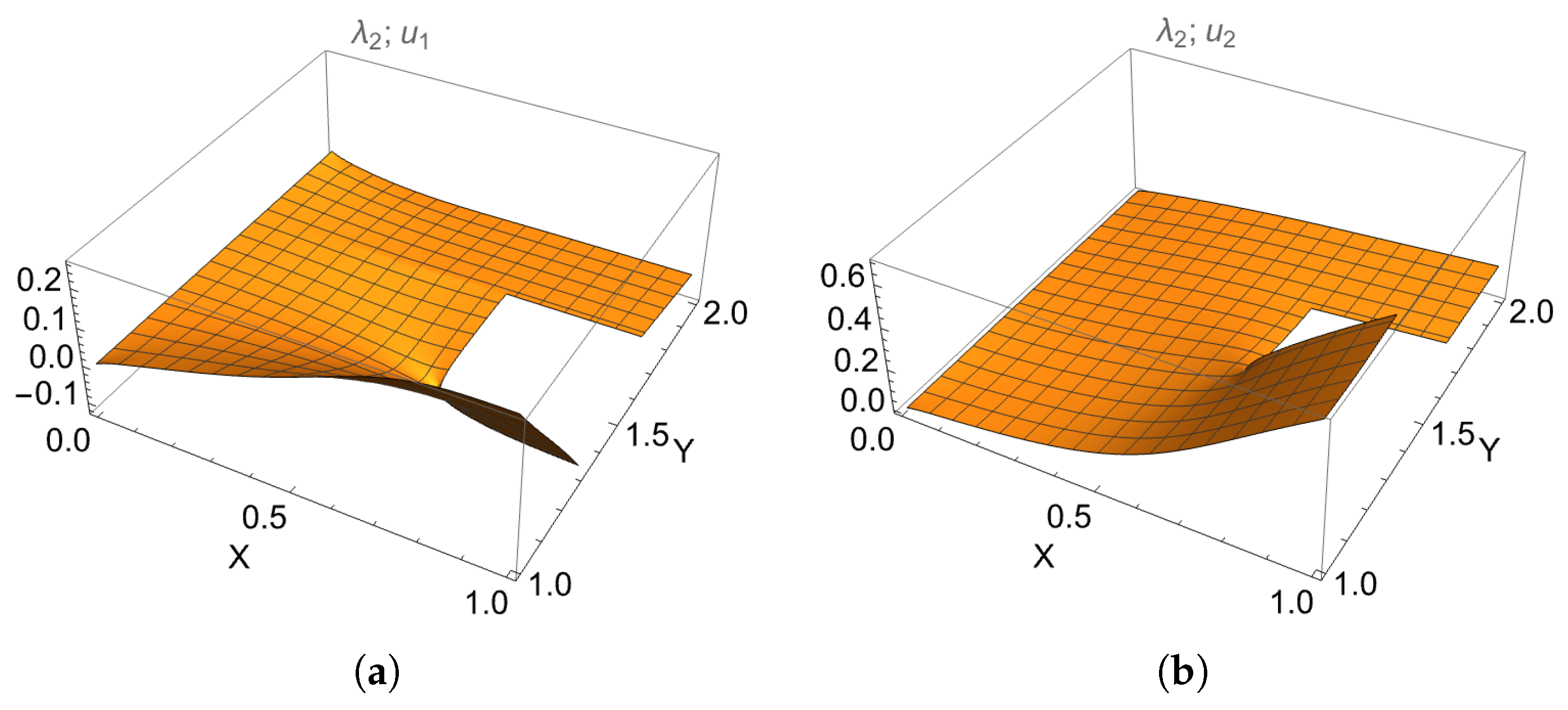
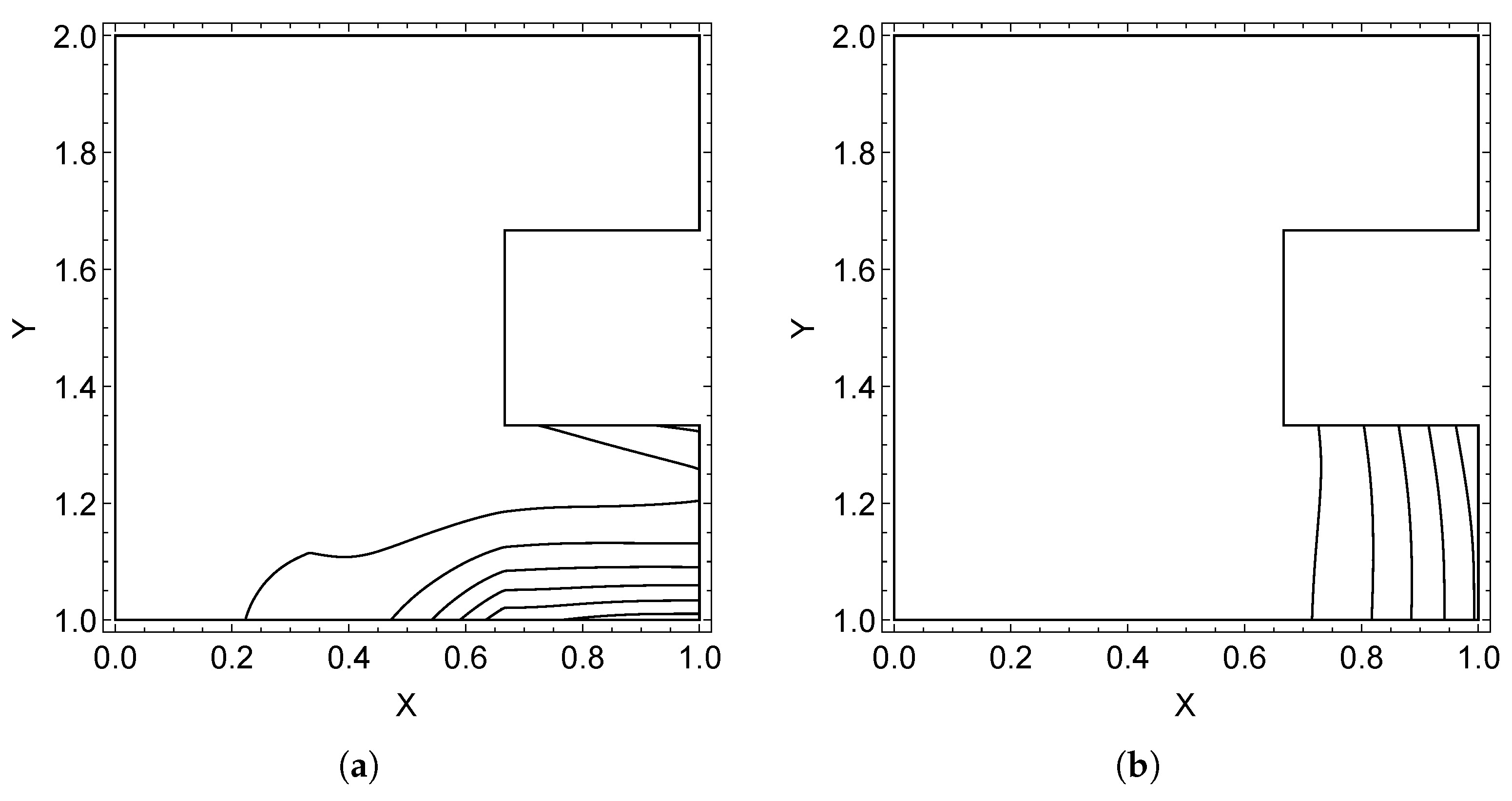
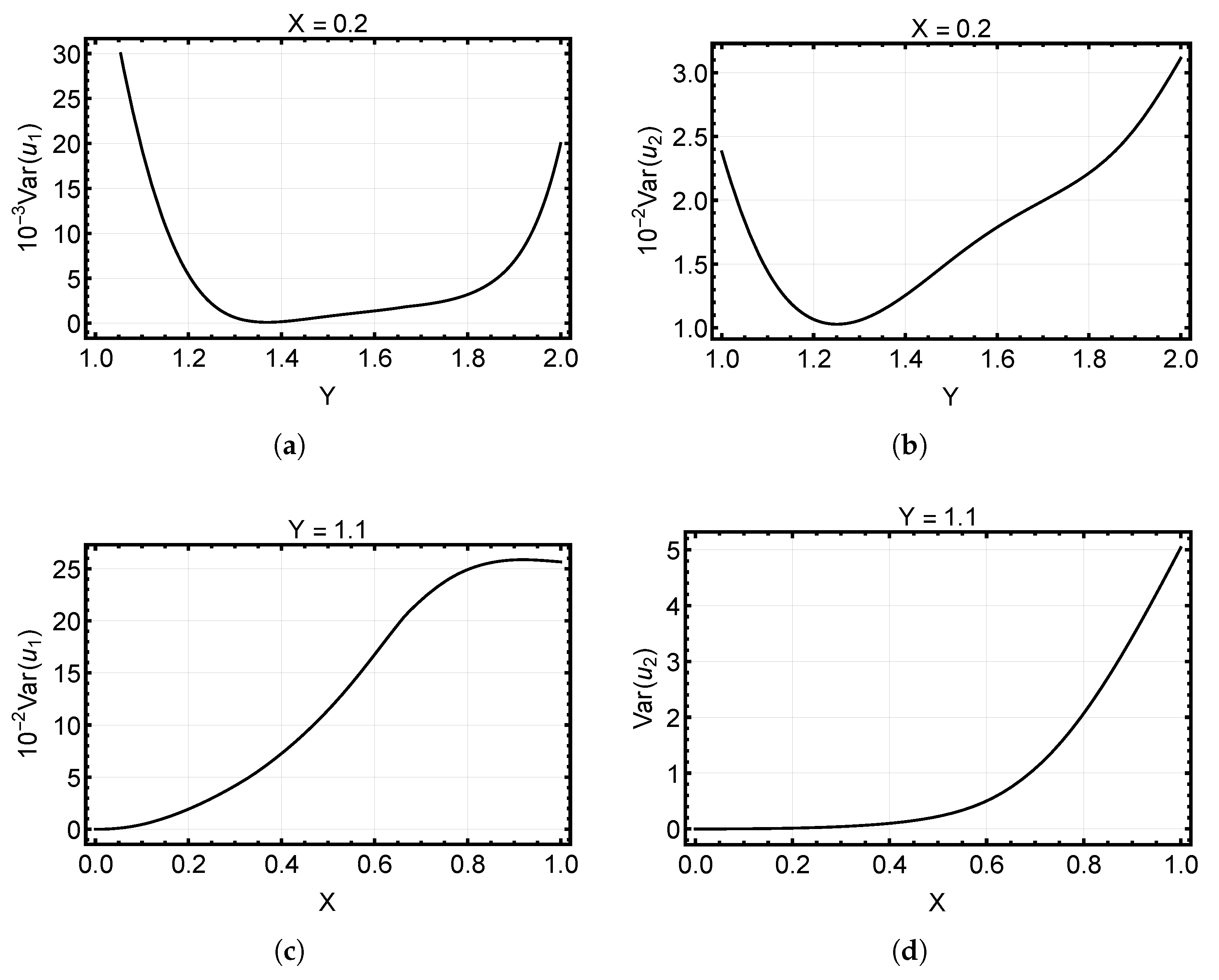
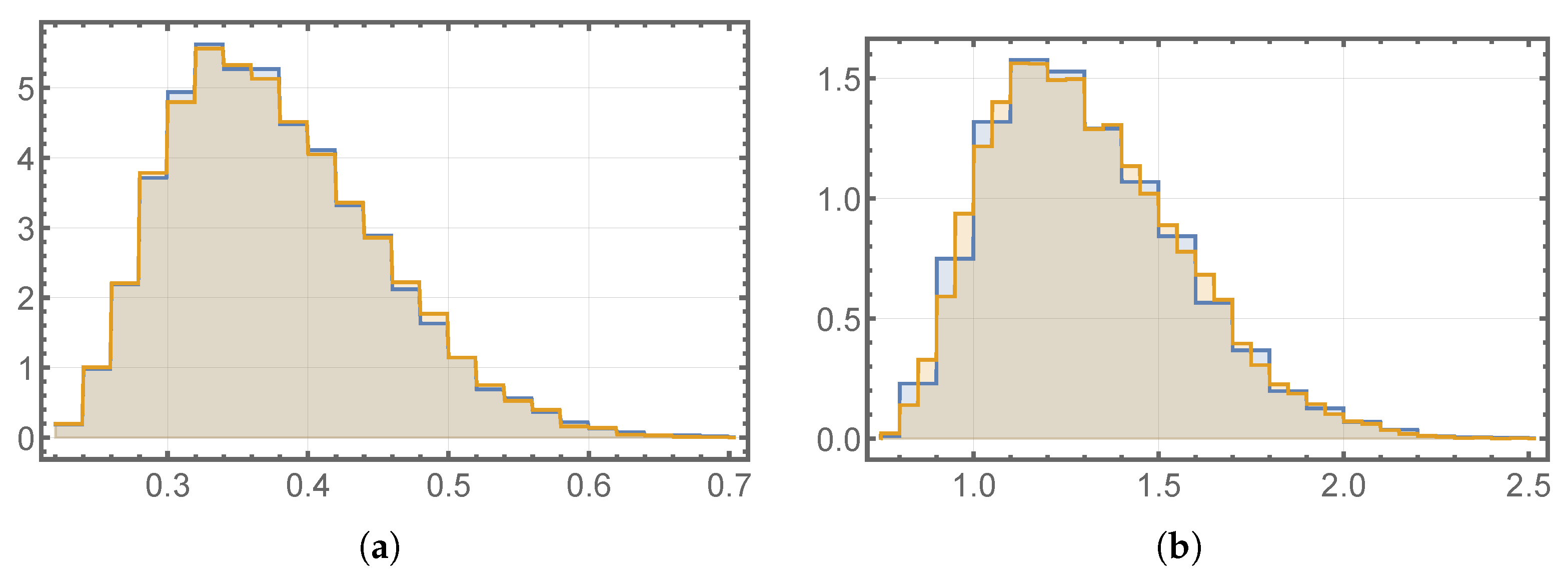
6.1. Case 1: Three Regions

The first configuration has three layers of regions, with the following decay rates: ${\zeta }_1={\zeta }_3=2$, ${\zeta }_2=3$, ${\epsilon }_i=1/100$, $i=1,2,3$. Using the data in Examples 1 and 2, in the tensor product form the effective stochastic dimension is $10\times 4\times 10=400$ including the constant or deterministic dimension, and the number of multi-indices is 1280 (see Figure 2). The expected solution and variance are shown in Figure 3 and Figure 4 above. The computed norms of the quantities of interest are provided in

Table 1. Computed quantities of interest. As expected, the norms of the expected solutions differ only marginally, whereas the difference in variance reflects the different underlying models of material uncertainty.

Case	Component	${\parallel \mathbf{Var}\left(\mathit{·}\right)\parallel }_2$	${\parallel \mathbb{E}\left(\mathit{·}\right)\parallel }_2$	${\parallel \mathbb{E}\left(\mathit{·}\right)\parallel }_0^1$
1	$u_1$	0.0155271	0.377051	2.92399
	$u_2$	0.161968	1.30773	3.50161
1 (TD)	$u_1$	0.0156688	0.377103	2.92443
	$u_2$	0.163275	1.30790	3.50212
2	$u_1$	0.102814	0.433761	3.3545
	$u_2$	1.00627	1.49574	4.0166

. For realizations of the Young’s modulus, see Figure 5. In Figure 6, convergence of the pseudoenergies of the Legendre coefficients has been illustrated in three ways: in log–log scale unsorted or in order, then sorted by magnitude, and finally in log scale sorted by magnitude. In the log-scale plot the algebraic, exponential, and super exponential regions can be identified. Due to transition phases, accurate determination of respective intervals is difficult. The algebraic region sets the bound for the asymptotic convergence rate and is naturally the most important. The super exponential region contains basis polynomials that do not contribute to the overall solution, and could be removed from the basis in the refined solution. It is an indication of the effectiveness of the selection algorithm that even with the naive tensor product structure of the global basis, only a small fraction of the selected modes have negligible contributions.

As mentioned above, visualization of the Legendre modes is straightforward. In Figure 7 and Figure 8, the extremal modes as measured with the pseudoenergy are shown. Interestingly, in Figure 7a there appears to be strong interaction of the mode with the corner singularity. One of the questions for further studies will be to investigate the relationship between the graded mesh and the Legendre coefficients.

6.2. Case 2: Eight Regions

The second configuration has eight regions, with the following decay rates: ${\zeta }_i=2$, ${\epsilon }_i=1/10$, $i=1,\cdots ,8$. For the realizations of the Young’s modulus, see Figure 9.

As the expected solution is very similar to that of the previous configuration, only the variance plots are shown in Figure 10 and Figure 11. Note that the location of the maximal variance has shifted. This is not surprising, as the underlying model is different. Nevertheless, this does indicate that the method itself is performing as expected. As for the previous case, the computed norms of the quantities of interest are provided in Table 1.

The contour plots are useful in verifying the line projection plots of the variance in Figure 12. As the underlying formulation is continuous, there are no jumps in the variance, although the effects of the multiple regions can immediately be identified from the plots. This kind of information is valuable when the sensitivity of the design with respect to individual parts is estimated a priori.

6.3. Comparative Analysis

Even though both configurations share the same deterministic part, the random material models are different, and hence direct comparison of the results is not well motivated. The computed norms of quantities of interest in Table 1 indicate that the expected solution is indeed not significantly influenced by the differences in the underlying material models. For variance, the situation is of course different.

Interestingly, the asymptotic convergence rates of the Legendre coefficients shown in Figure 13a–c do not differ greatly. The data fit well within the “best guess” asymptotic rates (with positive signs for convergence): $L^2\left(·\right)\sim H_0^1\left(·\right)\sim 1/2$ and ${\parallel u\parallel }_{A_0}\sim 1$. An additional test with Galerkin with a total degree ($\mathtt{isoTD}(·,K=2)$) truncation scheme is included as well. In Figure 13d, the heuristic selection algorithm (Andreev) is compared with the total degree one using the Legendre coefficients. Using the gap between the respective graphs as a rough error measure, it can be concluded that while the heuristic is not optimal, it is very good. It is worth remembering that Figure 6a indicates that it is not simple to estimate the individual contributions of modes.

The asymptotic rate estimates are useful in two ways; within one configuration, it is possible to estimate the computational resources for some guaranteed level of accuracy (or confidence), while in the context of this study, ranking of problems (again by computational complexity) is feasible.

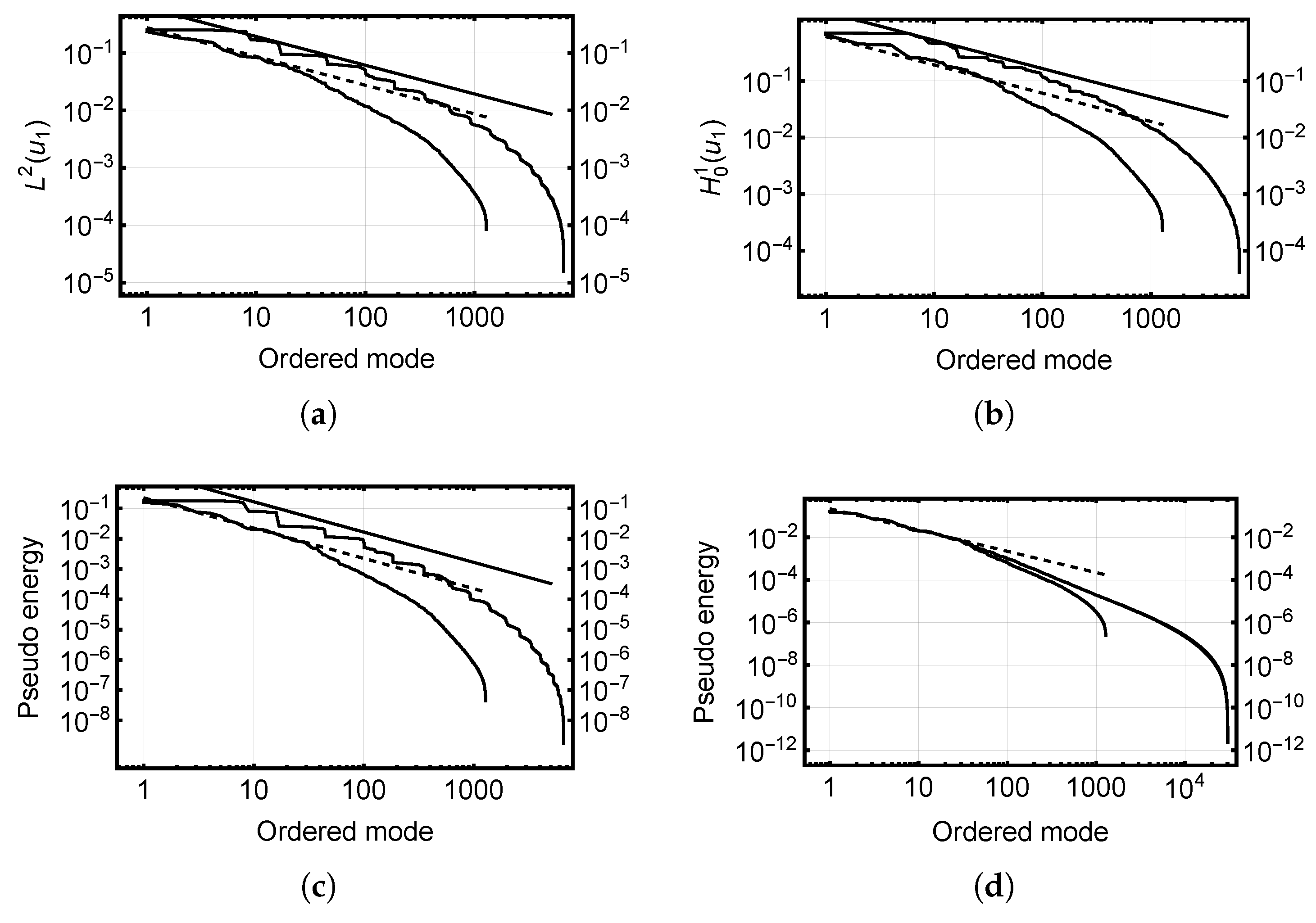
6.3.1. Verification Study of Case 1

The results using the proposed approach were verified using both Monte Carlo and quasi-Monte Carlo methods. In Figure 14 the convergence graphs of Monte Carlo solutions and the Galerkin solutions using exactly the same sampled parameter values are shown. As can be seen, the error is comparable to the standard $\sigma /\sqrt{N}$ estimate, where the standard deviation is taken as that obtained using the Galerkin solution. As there are no guarantees for pointwise convergence, it is useful to visualize the respective distributions of the quantities of interest in Figure 15. With high confidence, we can conclude that the proposed method and the MC solution agree.

The QMC results have been computed using rule 32001-1024-1048576.3600 (one of Kuo’s lattices [14]), with the average values per quadrature point taken over eight random shifts. The obtained values are for $N=2^{13}$ points $\parallel \mathbb{E}\left(u_1\right){\parallel }_2=0.337314$ and $\parallel \mathbb{E}\left(u_1\right){\parallel }_2=1.30909$, both of which are within the theoretical error bounds of $\sim 1/N$.

6.3.2. Time and Space Complexity

On a modern Mac M1 Max with eight cores and 64GB of RAM, in the case with eight regions integration of the system took one hour using straightforward parallel implementation, while the linear solver took ten hours for seven iterations of the conjugate gradient method. The residual tolerance for the solver was $1/10,000$, which for a system with over 17 million degrees of freedom is quite tight. Convergence is very fast in terms of steps due to the efficient preconditioning strategy; in fact, with tolerance of $1/100$ the time would have been halved. The solver was implemented with Mathematica [37,38].

While the integration phase required maximal memory capacity, the linear solver had a relatively small footprint due to the matrix-free variant of the iteration used. More detailed profiling of the iterative solver is beyond the scope of this study.

7. Conclusions

Solving problems with multiple spatially uncertain material parameters can be cast into the standard stochastic Galerkin framework. As always, selection of the appropriate basis for the Galerkin approximation is central. Here, a hybrid approach is introduced; each individual region with a random material parameter has its own efficient stochastic basis, yet the final global basis is taken to be a tensor product of these bases. Analysis of the convergence of the expansion coefficients shows that this strategy is surprisingly efficient, producing only a small fraction of basis polynomials with vanishingly small contributions in the quantities of interest.

The solution of the linear systems has been performed with the standard conjugate gradient method using a block-diagonal preconditioner adapted to the special structure of the system. Both the preconditioner and the matrix-vector product have natural matrix-free formulations. The method is highly efficient in terms of the number of steps, however, real time complexity depends on other aspects, including the convergence criteria.

The two sample configurations considered here are sufficiently different to lead to different variance in the solutions in both magnitude and spatial localization. This underlines the usefulness of the post-processing techniques directly available within the stochastic Galerkin methods.

This method appears to be very promising indeed. One of the intended immediate future application areas is multi-panel structures such as assembled shell structures.

References

1. Ghanem, R.; Spanos, P. Stochastic Finite Elements: A Spectral Approach; Dover Publications, Inc.: Mineola, NY, USA, 2003. [Google Scholar]
2. Schenk, C.A.; Schuëller, G.I. Uncertainty Assessment of Large Finite Element Systems; Lecture Notes in Applied and Computational Mathematics; Springer: Berlin/Heidelberg, Germany, 2005; Volume 24. [Google Scholar]
3. Babuška, I.; Nobile, F.; Tempone, R. A stochastic collocation method for elliptic partial differential equations with random input data. SIAM J. Numer. Anal. 2007, 45, 1005–1034. [Google Scholar] [CrossRef]
4. Schwab, C.; Gittelson, C.J. Sparse Tensor Discretizations of High-Dimensional Parametric and Stochastic PDEs. Acta Numer. 2011, 20, 291–467. [Google Scholar] [CrossRef] [Green Version]
5. Xiu, D. Numerical Methods for Stochastic Computations: A Spectral Method Approach; Princeton University Press: Princeton, NJ, USA, 2010. [Google Scholar]
6. Sullivan, T.J. Introduction to Uncertainty Quantification; Texts in Applied Mathematics; Springer: Berlin/Heidelberg, Germany, 2015; Volume 63. [Google Scholar]
7. Soize, C. Uncertainty Quantification; Interdisciplinary Applied Mathematics; Springer: Berlin/Heidelberg, Germany, 2017; Volume 47. [Google Scholar]
8. Wu, L.; Nguyen, V.D.; Adam, L.; Noels, L. An inverse micro-mechanical analysis toward the stochastic homogenization of nonlinear random composites. Comput. Methods Appl. Mech. Eng. 2019, 348, 97–138. [Google Scholar] [CrossRef] [Green Version]
9. Kumar, D.; Koutsawa, Y.; Rauchs, G.; Marchi, M.; Kavka, C.; Belouettar, S. Efficient uncertainty quantification and management in the early stage design of composite applications. Compos. Struct. 2020, 251, 112538. [Google Scholar] [CrossRef]
10. Mathew, T.V.; Pramod, A.; Ooi, E.T.; Natarajan, S. An efficient forward propagation of multiple random fields using a stochastic Galerkin scaled boundary finite element method. Comput. Methods Appl. Mech. Eng. 2020, 367, 112994. [Google Scholar] [CrossRef]
11. Ostoja-Starzewski, M. Material spatial randomness: From statistical to representative volume element. Probabilistic Eng. Mech. 2006, 21, 112–132. [Google Scholar] [CrossRef]
12. Charrier, J.; Scheichl, R.; Teckentrup, A.L. Finite element error analysis of elliptic PDEs with random coefficients and its application to multilevel Monte Carlo methods. SIAM J. Numer. Anal. 2013, 51, 322–352. [Google Scholar] [CrossRef] [Green Version]
13. Kuo, F.Y.; Schwab, C.; Sloan, I.H. Quasi-Monte Carlo Finite Element Methods for a Class of Elliptic Partial Differential Equations with Random Coefficients. SIAM J. Numer. Anal. 2012, 50, 3351–3374. [Google Scholar] [CrossRef]
14. Kuo, F.Y.; Nuyens, D. Application of Quasi-Monte Carlo Methods to Elliptic PDEs with Random Diffusion Coefficients: A Survey of Analysis and Implementation. Found. Comput. Math. 2016, 16, 1631–1696. [Google Scholar] [CrossRef] [Green Version]
15. Kuo, F.Y.; Nuyens, D. Application of Quasi-Monte Carlo Methods to PDEs with Random Coefficients—An Overview and Tutorial. In Monte Carlo and Quasi-Monte Carlo Methods; Owen, A.B., Glynn, P.W., Eds.; Springer International Publishing: Cham, Switzerland, 2018; pp. 53–71. [Google Scholar]
16. Bungartz, H.J.; Griebel, M. Sparse grids. Acta Numer. 2004, 13, 1–123. [Google Scholar] [CrossRef]
17. Lang, J.; Scheichl, R.; Silvester, D. A fully adaptive multilevel stochastic collocation strategy for solving elliptic PDEs with random data. J. Comput. Phys. 2020, 419, 109692. [Google Scholar] [CrossRef]
18. Bieri, M.; Andreev, R.; Schwab, C. Sparse Tensor Discretization of Elliptic SPDEs. SIAM J. Sci. Comput. 2009, 31, 4281–4304. [Google Scholar] [CrossRef]
19. Klawonn, A.; Pavarino, L.F.; Rheinbach, O. Spectral element FETI-DP and BDDC preconditioners with multi-element subdomains. Comput. Methods Appl. Mech. Eng. 2008, 198, 511–523. [Google Scholar] [CrossRef]
20. Eigel, M.; Gruhlke, R. A local hybrid surrogate-based finite element tearing interconnecting dual-primal method for nonsmooth random partial differential equations. Int. J. Numer. Methods Eng. 2021, 122, 1001–1030. [Google Scholar] [CrossRef]
21. Khan, A.; Powell, C.E.; Silvester, D.J. Robust Preconditioning for Stochastic Galerkin Formulations of Parameter-Dependent Nearly Incompressible Elasticity Equations. SIAM J. Sci. Comput. 2019, 41, A402–A421. [Google Scholar] [CrossRef]
22. Bespalov, A.; Praetorius, D.; Ruggeri, M. Convergence and rate optimality of adaptive multilevel stochastic Galerkin FEM. IMA J. Numer. Anal. 2021, 42, 2190–2213. [Google Scholar] [CrossRef]
23. Heinlein, A.; Klawonn, A.; Lanser, M. Adaptive Nonlinear Domain Decomposition Methods; Technical Report for Center for Data and Simulation Science: Cologne, Germany, 2021. [Google Scholar]
24. Slaughter, W.S. The Linearized Theory of Elasticity; Birkhäuser: Basel, Switzerland, 2002. [Google Scholar]
25. Ghanem, R.G.; Doostan, A. On the construction and analysis of stochastic models: Characterization and propagation of the errors associated with limited data. J. Comput. Phys. 2006, 217, 63–81. [Google Scholar] [CrossRef]
26. Das, S.; Ghanem, R.; Finette, S. Polynomial chaos representation of spatio-temporal random fields from experimental measurements. J. Comput. Phys. 2009, 228, 8726–8751. [Google Scholar] [CrossRef]
27. Szabo, B.; Babuska, I. Finite Element Analysis; John Wiley & Sons: Hoboken, NJ, USA, 1991. [Google Scholar]
28. Schwab, C. p- and hp-Finite Element Methods; Oxford University Press: Oxford, UK, 1998. [Google Scholar]
29. Soize, C.; Ghanem, R. Physical Systems with Random Uncertainties: Chaos Representations with Arbitrary Probability Measure. SIAM J. Sci. Comput. 2004, 26, 395–410. [Google Scholar] [CrossRef] [Green Version]
30. Xiu, D.; Karniadakis, G.E. The Wiener-Askey Polynomial Chaos for Stochastic Differential Equations. SIAM J. Sci. Comput. 2002, 24, 619–644. [Google Scholar] [CrossRef]
31. Rosenblatt, M. Remarks on multivariate transformation. Ann. Math. Stat. 1952, 23, 470–472. [Google Scholar] [CrossRef]
32. Bieri, M. Sparse Tensor Discretizations of Elliptic PDEs with Random Input Data. Ph.D. Thesis, ETH Zürich, Zürich, Switzerland, 2009. [Google Scholar]
33. Beck, J.; Tempone, R.F.; Nobile, F.; Tamellini, L. On the optimal polynomial approximation of stochastic PDEs by Galerkin and collocation methods. Math. Models Methods Appl. Sci. 2012, 22, 1250023. [Google Scholar] [CrossRef] [Green Version]
34. Bäck, J.; Nobile, F.; Tamellini, L.; Tempone, R.F. Stochastic Spectral Galerkin and Collocation Methods for PDEs with Random Coefficients: A Numerical Comparison. In Spectral and High Order Methods for Partial Differential Equations; Lecture Notes in Computational Science and, Engineering; Hesthaven, J.S., Ronquist, E.M., Eds.; Springer: Berlin/Heidelberg, Germany, 2011; Volume 76, pp. 43–62. [Google Scholar] [CrossRef]
35. Powell, C.E.; Elman, H.C. Block-diagonal preconditioning for spectral stochastic finite-element systems. IMA J. Numer. Anal. 2008, 29, 350–375. [Google Scholar] [CrossRef] [Green Version]
36. Golub, G.H.; van Loan, C.F. Matrix Computations, 4th ed.; JHU Press: Baltimore, MD, USA, 2013. [Google Scholar]
37. Wolfram Research. Mathematica, Version 13.0.1; Wolfram Research: Champaign, IL, USA, 2021. [Google Scholar]
38. Hakula, H.; Tuominen, T. Mathematica implementation of the high order finite element method applied to eigenproblems. Computing 2013, 95, 277–301. [Google Scholar] [CrossRef]
Figure 1. Model problem configuration. The computational domain has three layers and eight regions. The traction loading that acts on the inner boundary segment is indicated with arrows. The boundary at x = 0 is fully clamped, while all other boundaries are free. (a) CAD model of the domain; (b) computational domain.
Applmech 03 00055 g001
Figure 2. Graded mesh used in all simulations. N 1 and N 2 refer to the dimensions of the linear systems of the two configurations, respectively, and N T D is the dimension of the first case with the total degree selected and isoTD ( · , K = 2 ) . (a) Geometrically graded mesh used in all simulations and (b) discretization data. Sizes of the mesh components and stochastic basis used at deterministic p = 4 .
Applmech 03 00055 g002
Figure 3. Three layers of uncertain materials. Examples of expected solutions. Temperature scale with zero level at the boundary x = 0 . (a) E ( u 1 ) [ 1.80 , 0.83 ] , (b) E ( u 2 ) [ 4.85 , 0 ] . Decay rates: ζ 1 = ζ 3 = 2 , ζ 2 = 3 , ε i = 1 / 100 , i = 1 , 2 , 3 .
Applmech 03 00055 g003
Figure 4. Three layers of uncertain materials. Examples of computed variance. Temperature scale with zero level at the boundary x = 0 . (a) Var ( u 1 ) [ 0 , 0.11 ] , (b) Var ( u 2 ) [ 0 , 0.83 ] . Decay rates: ζ 1 = ζ 3 = 2 , ζ 2 = 3 , ε i = 1 / 100 , i = 1 , 2 , 3 .
Applmech 03 00055 g004
Figure 5. Three regions. Realizations of the Young’s modulus in different configurations. The region with index 1 is set to zero for visualization purposes only. (a) Dimension index i = { 1 , 3 , 4 } , (b) Dimension index i = { 4 , 2 , 3 } .
Applmech 03 00055 g005
Figure 6. Three regions of uncertain materials. Convergence of the Legendre coefficients in pseudoenergy. In the log-scale plot, the algebraic, exponential, and super exponential regions can be identified. Due to transition phases, accurate determination of respective intervals is difficult. (a) Unsorted; observed pseudoenergy per stochastic basis polynomial (loglog). (b) Sorted; observed pseudoenergy per stochastic basis polynomial sorted by magnitude (loglog). (c) Sorted; observed pseudoenergy per stochastic basis polynomial sorted by magnitude in log-scale.
Applmech 03 00055 g006
Figure 7. Three regions of uncertain materials. Visualization of the Legendre coefficients of the stochastic modes with the highest pseudoenergies, λ 2 = L 1 1 L 1 6 . Here, λ 2 indicates that the mode was selected as the 2nd; (a) λ 2 ( u 1 ) and (b) λ 2 ( u 2 ) .
Applmech 03 00055 g007
Figure 8. Three regions of uncertain materials. Visualization of the Legendre coefficients of the stochastic modes with the smallest pseudoenergies, λ 1103 = ( L 1 1 ) 2 ( L 2 1 ) ( L 1 4 ) 2 . Here, λ 1103 indicates that the mode was selected as the 1103th; (a) λ 1103 ( u 1 ) and (b) λ 1103 ( u 2 ) .
Applmech 03 00055 g008
Figure 9. Eight regions. Realizations of the Young’s modulus in different configurations. The region with index 1 is set to zero for visualization purposes only. (a) Dimension index i = { 1 , 1 , 1 , 2 , 2 , 3 , 3 , 2 } , (b) Dimension index i = { 1 , 2 , 2 , 2 , 3 , 2 , 3 , 2 } .
Applmech 03 00055 g009
Figure 10. Eight regions of uncertain materials. Unit traction force acting on u 2 along the horizontal segment at y = 4 / 3 . Temperature scale with zero level at the boundary x = 0 . (a) Var ( u 1 ) [ 0 , 0.78 ] and (b) Var ( u 2 ) [ 0 , 5.40 ] . Decay rates: ζ i = 2 , ε i = 1 / 10 , i = 1 , , 8 .
Applmech 03 00055 g010
Figure 11. Eight regions of uncertain materials. Contour plots of the variance of the vector field components. The zero level is at x = 0 in both pictures. The plots are not directly comparable, as Var ( u 1 ) 2   = 0.1 < Var ( u 2 ) 2 = 1.0 . (a) Var ( u 1 ) and (b) Var ( u 2 ) .
Applmech 03 00055 g011
Figure 12. Eight regions of uncertain materials. Detail plots of the variance along cuts over the deterministic computational domain. Although there are jumps in the realizations of the random material field, the solution method is continuous. (a) Var ( u 1 ) , (b) Var ( u 2 ) , (c) Var ( u 1 ) , (d) Var ( u 2 ) .
Applmech 03 00055 g012
Figure 13. Convergence comparison between the two configurations: Computed quantity of interest (sorted in magnitude) vs. the basis polynomials. For both norms, the rate is = 1 / 2 , and for the pseudoenergy = 1 . The solid straight line is the estimated upper bound for Case 2, and the dashed one for Case 1. Notice that the number of poorly performing bases is a small fraction of the total in both cases. In (d), both solid curves represent Case 1, with the longer one corresponding to the total degree selection. (a) L 2 ( u 1 ) , (b) H 0 1 ( u 1 ) , (c) u A 0 , (d) u A 0 .
Applmech 03 00055 g013
Figure 14. Convergence graph of absolute value of the error of the Monte Carlo (Black) and sampled Galerkin (Red) solutions. The upper bound is the standard σ / N , where σ is computed using Table 1. (a) L 2 ( u 1 ) : Monte Carlo convergence and (b) L 2 ( u 2 ) : Monte Carlo convergence.
Applmech 03 00055 g014
Figure 15. Distributions of the quantities of interest of the Monte Carlo (Orange) and sampled Galerkin (Blue) solutions. The agreement is excellent. The x-axis is the observed value and the y-axis is the normalized pseudofrequency; the area under the graph is equal to one. (a) L 2 ( u 1 ) : Monte Carlo convergence and (b) L 2 ( u 2 ) : Monte Carlo convergence.
Applmech 03 00055 g015