2.4.1. Computational Model for Stationary Heat Transfer
The investigation of the heat transfer coefficient is based on the assumption that a control volume of the flat plate specimen can be represented in a numerical model, which is able to cover the governing material laws for the thermal processes, the influencing material, properties and thermal boundary conditions. Based on the transient heat transfer Equation (
1), the stationary case can be defined for
in a discrete homogenised material domain to
where
is the effective heat conductivity tensor of domain
,
is the stationary temperature at a spatial point in domain
, and
represents the sum of the local volumetric heat sources and sinks (compare former work of the authors [
11]). The discrete, stationary heat transfer problem can be solved by the finite element method for arbitrary geometries using, e.g., Comsol Multiphysics, which is used for this work in version 6. Comsol Multiphysics is a commercial software used for coupled physics simulations based on the finite element method, comprising also the heat transfer equation and all related modelling tools. Furthermore, MATLAB is used to analyse measured data and transfer such data to Comsol Multiphysics via MATLAB LiveLink. The model boundary conditions and assumptions, e.g., homogenisation methods for GF and CF composite plies, are defined such that the resulting temperature field can represent the state identified by experimental investigations at the flat plate specimen (see
Section 2.4.2).
However, the experimental work described previously represents a transient heat-up process until a stationary heat transfer is reached over time. The stationary case is given at that point of time, when the change of maximum temperature at the surface of the specimen
is minimal. This condition is defined here by the point of time when the minimum of the empirical variance
(called “variance” hereinafter) of the desired quantity is found. Therefore the variance is computed as
where
denotes a point in time in the measurement interval,
is the maximum temperature of the field at time
,
is the mean value of related temperature maxima, and
is the chosen data interval over time with a length of 40 data steps. This length corresponds to a time interval of 20 s, because the scanning frequency was set to 2 Hz. The variance is computed for the total number of
k time intervals in the dataset. The stationary maximum temperature is then
, where
is the point in time where the minimum of
is found. With this definition,
can be compared with the solution of the stationary temperature field of the model.
However, the computed temperature field is dependent on the boundary conditions, which are defined together with further model assumptions in the following subsection.
2.4.2. Assumptions and Boundary Conditions
As described in
Section 2.1 and
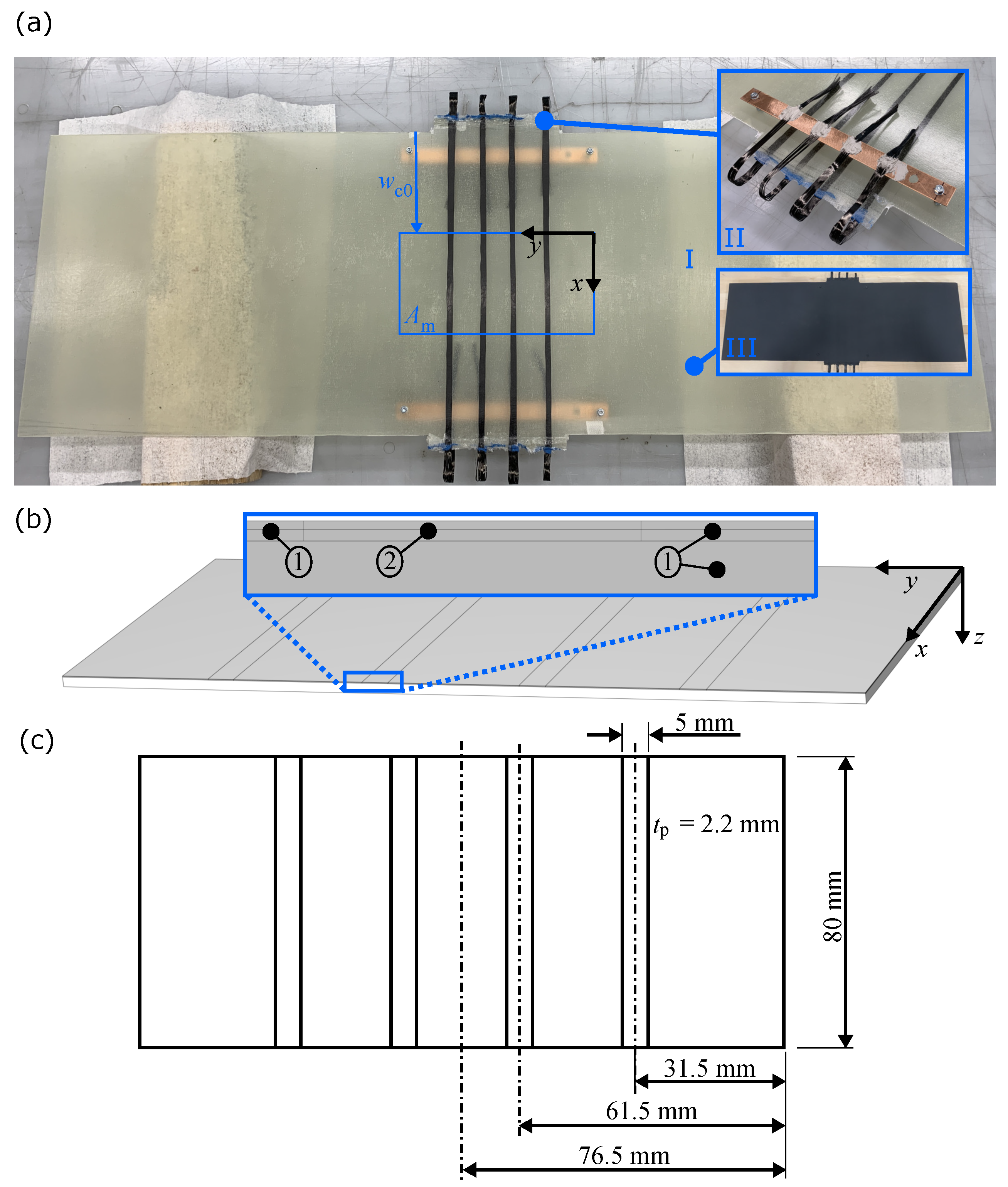
Section 2.2, the control volume is related to the measured surface area
in
-coordinates. The control volume is shown again in
Figure 5a with indicated boundaries, which are named by the respective coordinate axis surface normals (
, related to
x,
y,
z coordinates, respectively). In
Figure 5b, a closeup of the three different domains is given:
—the passive CF composite layers,
—the active CF composite layers, and
—the passive glass fibre composite layers. “Active” indicates here that Joule heating by current conduction is applied to this domain, whereas the passive domains are electrically inactive.
The domains
and
are separated only to define the active volume, where Joule heat is emitted. The volume ratio of these domains is defined as follows:
where
are the respective domain volumes and
is the carbon fibre volume ratio in the top layer of the laminate (compare
Table 3 and
Figure 5). Accordingly,
is exactly the volume of the CFs applied for Joule heating (4× 24k carbon fibre rovings, compare
Section 2.2). This definition is reasonable, as the volume (length and cross sectional area) define the effective resistance of the carbon fibres, thus governing Joule heat emission [
1].
The material properties are defined as effective properties related to thermal conductivities resulting from fibre orientation in the laminate (see
Table 3). According to earlier work of Schutzeichel et al. [
1],
and
are assumed to be thermally transversal isotropic, where the longitudinal direction of the unidirectional (UD) CFs is related to the
x-axis here. The GF composite domain is effectively isotropic, as the thermal conductivity is identical for all directions. This can be reduced to the low thermal conductivities of both GF and epoxy resin.
The domain related fibre volume fractions
, resulting effective thermal conductivities
, and the specific electrical resistances
for the single domains are given in
Table 3. The indices indicate the constituents as well as the effective direction or plane. It should be noted that the fibre volume fractions were determined by thermogravimetric analysis of material specimens taken from the flat plate after the described measurements were finished. As the CF and GF composite domains are two-phase material domains, the rule of mixture (ROM) is used for longitudinal ‖ as well as transversal ⊥ isotropic effective properties, which results in proper measures according to [
11]. To apply current conduction only to
, specific electrical resistances of
and
are set to infinity. All constituents’ properties feeding into the effective properties are given in
Appendix A.
In addition to domain and material property definitions, the BCs are essential in this approach to achieve a proper calculation of the heat transfer coefficient. The thermal BCs should represent the conditions during the experimental investigation (see
Section 2.3.2) and are defined as follows:
where
indicates a periodic BC,
indicates a boundary inward heat flux with inward surface normal
in z-direction,
A is the local surface area,
h is the HTC,
is the Stefan–Boltzmann constant, and
is the emissivity of the surface. Indices c and r denote convective and radiative, respectively. All conditions are related to the boundaries defined in
Figure 5 for all domains
–
. The back side of the control volume is defined to be thermally adiabatic, which is reasonable, as the back side of the flat plate was covered to minimise thermal heat transfer (compare
Section 2.3.2). The periodic BC is chosen, as this volume element is repeatable along the
x direction of the flat plate. The boundaries
and
are defined to hold ambient temperature. Results of the experimental measurements indicate this assumption (see
Section 3.1). The BC on the surface
is defined as Newton’s convective heat transfer law (Equation (
14)). In addition to the convective heat transfer at the surface, thermal radiation is also assumed based on the defined emissivity
(see
Section 2.3.1).
Because ambient temperature
and the local surface area
A are known, the resulting temperature at the surface
is only controlled by the HTC
h. This enables the comparison of the measured maximum stationary temperature
from the experimental investigation (as defined in
Section 2.4.1) and the computed maximum temperature on the surface of the control volume
. Accordingly,
h is tailored in an iterative procedure to minimise the difference between
and
until a quality criterion
c is reached:
The criterion is defined here to hold , which is reasonable compared to the accuracy of the measured results.
In addition to the thermal BC and HTC evaluation, the volumetric heat source needs to be defined via Joule heating in the active carbon fibre domain
:
where
is the vector of the electric current density, which is given by a constant electrical current density
j and the inward surface normal
at surface
in domain
. The current density is related to the applied heating current
, set to the value measured during the experimental process (compare
Section 2.3.3), and the cross-sectional area of the four carbon fibre rovings
embedded in the flat plate, where
is based on the assumption of 24,000 fibres at each bundle with fibre diameter
[
35].
With this setup, the HTC is computed for all 25 stationary heat transfer cases defined in the experimental investigation. Furthermore, the HTC is evaluated towards the influence of the environmental conditions. All results are presented in the following section.

 ,
, 

