On the Free Vibration and the Buckling Analysis of Laminated Composite Beams Subjected to Axial Force and End Moment: A Dynamic Finite Element Analysis

Abstract

This work presents the bending–torsion coupled free vibration analysis of prestressed, layered composite beams subjected to axial force and end moment using the traditional finite element method (FEM) and dynamic finite element (DFE) techniques. Current trends in the literature, in terms of different types of modeling techniques and constraints, were briefly examined. The Galerkin-type weighted residual method was applied to convert the coupled differential equations of motion into a discrete problem using a polynomial interpolation function in the finite element method. In the dynamic finite element method, trigonometric shape functions were implemented to describe the equations in terms of nodal displacements. The eigenvalue problem resulting from the discretization along the length of the beam was solved in order to determine the system’s natural frequencies and modes. The results, showing the effects of axial load, end moment, and combined loading on natural frequencies, are discussed and are followed by some concluding remarks.

1. Introduction

Many situations arise in various engineering applications, ranging from terrestrial to aerospace structures, in which layered composite materials are used. The increasing interest in such layered structural elements is mainly because of their attractive properties, such as high specific stiffness and strength, formability into complex shapes, longer fatigue life, tailorable stiffness and strength, lower density, good buckling, and corrosion resistance, to name a few (see, for example, Jones [1] and Berthelot [2]). However, it is well known that composite structures can be placed under axial force and end moment simultaneously when used in the above applications. Additionally, they are very susceptible to flexural–torsional/lateral buckling and display complex vibrational behavior. Therefore, the accurate prediction of their stability limit states and dynamic characteristics is of fundamental importance in the design of composite structures. Changing the ply orientation and stacking sequence can lead to alterations of the composite material stiffness characteristics. For ply angles other than 0° and 90°, bending and torsion deformations are coupled, and this material coupling predominantly influences the natural frequencies and mode shapes of free vibration. Hashemi and Borneman [3] used a simplified beam model and the dynamic (frequency-dependent) finite element method (FEM) to investigate the coupling between bending and torsion in free vibration analysis of composite wings. Abramovich and Livshits [4], Jaehong and Kim [5], Chen et al. [6], and Jung et al. [7] used various numerical techniques, including Rayleigh–Ritz, Galerkin, and conventional FEM based on fixed (polynomial) interpolation functions to evaluate the element matrices. Among these methods, FEM is more commonly used, as it provides a general, systematic approach to formulate a system’s stiffness and mass matrices. The natural frequencies and modes of free vibration can then be found by solving the linear eigenvalue problem resulting from the assembly of element matrices and enforcing the system’s boundary conditions [8].

Modeling a homogeneous metallic beam using the finite element method is relatively straightforward; however, when using composite materials, their characteristics and behavior bring complexity to the system. This complexity, in addition to the time-consuming nature of FEM models when meshing and solving equations, has led many researchers to try analytical and semi-analytical approaches for early stages of design and optimization. The dynamic stiffness matrix (DSM) method was developed and employed to determine the free vibration response of various beam structures. The DSM was first proposed by Kolousek in the 1970s [9] for homogeneous Euler–Bernoulli beams and has since been continuously refined. In the 1990s, neglecting the shear and rotary inertia effects, Banerjee and his coworkers developed the DSM method for the vibration analysis of different homogeneous and composite beam models. The DSM model for a uniform Euler–Bernoulli composite beam, originally developed by Banerjee and Williams [10], and exploiting a general algorithm for computing the natural frequencies of elastic structures presented earlier by Wittrick and Williams [11], was then extended to the Timoshenko beam theory [12]. Later, Banerjee [13] further extended the DSM model to include axial force for different composite beam configurations. In all these works, the DSM models for composite beams were based on the exact member theory [11,12,13] and limited to simple geometries and special cases. Exploiting the conventional FEM formulation and the frequency-dependent approximation space from the DSM method, Hashemi and his coworkers developed the dynamic finite element (DFE) formulation to investigate the vibrations of various homogeneous and laminated composite beam configurations (see, e.g., [3,4,14,15]). However, to the best of the authors’ knowledge, a dynamic analysis of flexible prestressed composite beams subjected to combined axial load and end moment has not been reported in the available literature.

In this paper, a free vibration analysis of prestressed laminated composite and fiber-metal laminated (FML) beams subjected to axial force and end moment is presented. In addition to the material coupling between bending and torsion displacements caused by the ply angle in a laminated composite beam, which has been treated and reported many times in the literature, the system was also characterized by another geometric coupling resulting from the end moment, bringing more complexity to the vibration analysis of such prestressed structural elements. The equations of motion were introduced first, followed by mathematical formulations leading to the FEM and DFE models. Considering the illustrative examples, numerical tests were then performed to demonstrate the validity, precision, and practical applicability of the presented methods.

The DFE formulation presented in this paper used the analytical solutions of a simplified version of the uncoupled equations of motion as the shape functions of approximation space. As a result, the DFE model had a higher rate of convergence in comparison with the conventional FEM model. This could save a large amount of computational time and improve the accuracy of solutions in the design process, especially in large-scale designs. The FEM method was developed for the sake of comparison in the cases studied, where experimental or analytical results did not exist.

The structure of the paper is as follows: Section 2 presents the concept of coupled, linear, undamped, free vibration of a prestressed laminated composite beam, followed by the expressions for the Galerkin-type integral form of the governing differential equations. Then, two composite beam conventional and dynamic frequency-dependent FEM formulations are presented. In Section 3, the application of the presented formulations to the free vibration analysis of a cantilevered, single-layer glass–epoxy composite beam (3.1) and a three-layered fiber-metal laminated (FML) beam (3.2) is presented. In Section 4, a discussion of the results obtained is provided, followed by final conclusions summarizing the most important achievements of the presented work.

2. Materials and Methods

Consider a slender laminated composite beam of length L and its solid rectangular cross section, as shown in Figure 1. The material bending–torsion coupling behavior usually present in composite materials is due to the unbalanced layup. The beam is characterized by the effective (equivalent) bending rigidity, EI; the torsional rigidity, GJ; and the material bending–torsion coupling rigidity, K (see [10] for more information on coupling rigidity). A symmetric configuration consists of symmetry in the fiber orientations and thicknesses with respect to the mid-plane of the laminate.

Neglecting the shear, rotary inertia, and warping effects, the Euler–Bernoulli bending and St. Venant torsion beam theories are used, where the flexural displacement is denoted by w and θ is used to denote the twist angle. Differential equations of motion governing the undamped, linear, coupled bending–torsion vibration of the system can be developed by writing the equilibrium equations for an infinitesimal element of the system. The development of the system’s governing differential equations is based on the assumptions of linearly elastic material, small displacements, and rectangular cross-sectional area (i.e., two axes of symmetry), with the dimensions being small compared to the span, and the transverse cross sections of the beam remaining plane and normal to the neutral axis during bending (Euler–Bernoulli bending beam theory). Furthermore, the beam’s torsional rigidity (GJ) is assumed to be very large compared with its warping rigidity (EΓ, and the ends are free to warp, i.e., they are in a state of uniform torsion. The total potential energy (U) of the beam is given by the following (the coupling rigidity terms are from the energy terms used in [16], the term for the end moment is from [17], and the rest of the terms are from [13]):

$$\begin{array}{l}U=\frac{1}{2}{\int }_0^L[b\left(D_{22}-\frac{D_{12}^2}{D_{11}}\right){\left(\frac{{\partial }^{2}w}{\partial x^2}\right)}^2+2b\left(D_{26}-\frac{D_{12}{D}_{16}}{D_{11}}\right)\left(\frac{{\partial }^{2}w}{\partial x^2}\right)\left(\frac{\partial \theta }{\partial x}\right)+4b\left(D_{66}-\frac{D_{16}^2}{D_{11}}\right){\left(\frac{\partial \theta }{\partial x}\right)}^2+P\{{\left(\frac{\partial w}{\partial x}\right)}^2+\left(\frac{I_P}{m}\right){\left(\frac{\partial \theta }{\partial x}\right)}^2\}\\ +M_{zz}\left(\frac{\partial w}{\partial x}\right)\left(\frac{\partial \theta }{\partial x}\right)]dx.\end{array}$$

(1)

Using the rigidities definitions from [13], Equation (1) can be rewritten as follows:

$$U=\frac{1}{2}{\int }_0^L[EI{\left(\frac{{\partial }^{2}w}{\partial x^2}\right)}^2+K\left(\frac{{\partial }^{2}w}{\partial x^2}\right)\left(\frac{\partial \theta }{\partial x}\right)+GJ{\left(\frac{\partial \theta }{\partial x}\right)}^2+P\left\{{\left(\frac{\partial w}{\partial x}\right)}^2+\left(\frac{I_P}{m}\right){\left(\frac{\partial \theta }{\partial x}\right)}^2\right\}+M_{zz}\left(\frac{\partial w}{\partial x}\right)\left(\frac{\partial \theta }{\partial x}\right)]dx.$$

(2)

The total kinetic energy (T) is given by the following [18]:

$$T=\frac{1}{2}{\int }_0^L\left[m{\left(\frac{\partial w}{\partial t}\right)}^2+I_P{\left(\frac{\partial \theta }{\partial t}\right)}^2\right]dx.$$

(3)

Based on Hamilton’s principle, for Lagrangian (L = T − U), ${\int }_{t_1}^{t_2}L dt$ is stationary between any arbitrary intervals of time (t₁, t₂), which means:

$$\delta {{\displaystyle \int }}_{t_2}^{t_2}\left(T-U\right)dt=0$$

(4)

where δ is the variational operator. By substituting 2 and 3 into 4, integrating each term by parts, using the δ operator, knowing that δh and δθ are arbitrary, and finally collecting all the terms, the differential equations of motion governing the free undamped vibration of a prismatic, materially coupled, bending–torsion Euler–Bernoulli beam (EI = constant) subjected to constant axial force (P) and end moment (M_zz) are written as:

$$EI\frac{{\partial }^{4}w}{\partial x^4}+P\frac{{\partial }^{2}w}{\partial x^2}+K\frac{{\partial }^3\theta }{\partial x^3}+M_{zz}\frac{{\partial }^2\theta }{\partial x^2}-\left(\rho A\right)\frac{{\partial }^{2}w}{\partial t^2}=0$$

(5)

$$GJ\frac{{\partial }^2\theta }{\partial x^2}+\frac{P{I}_P}{A}\frac{{\partial }^2\theta }{\partial x^2}+K\frac{{\partial }^{3}w}{\partial x^3}+M_{zz}\frac{{\partial }^{2}w}{\partial x^2}-\rho I_P\frac{{\partial }^2\theta }{\partial t^2}=0$$

(6)

where GJ stands for the torsional rigidity, EI is the flexural rigidity, K represents the material bending–torsion coupling rigidity, ρ is the mass density, I_p represents the polar area moment of inertial per unit length, A stands for the cross-sectional area, x represents the distance spanning the beam, and t is time. The resultant internal bending moment, $M\left(x\right)$, shear force, S(x), and torsional torque, T(x), are given as:

$$M\left(x\right)=-EI{w}^{″}-K{\theta }^{\prime }$$

(7)

$$S\left(x\right)=EI{w}^{‴}+K{\theta }^{″}+M_{ZZ}{\theta }^{\prime }+P{w}^{\prime }$$

(8)

$$T\left(x\right)=GJ{\theta }^{\prime }+\frac{P{I}_P}{A}{\theta }^{\prime }+K{w}^{″}+M_{ZZ}{w}^{\prime }.$$

(9)

Based on the simple harmonic motion assumptions, the displacements can be assumed to have a sinusoidal variation (in time and frequency) as follows:

$$w\left(x,t\right)=W\mathit{sin}\omega t$$

(10)

$$\theta \left(x,t\right)=\overline{\theta } \mathit{sin}\omega t.$$

(11)

The sinusoidal variations from Equations (10) and (11) are then substituted into Equations (5) and (6) (i.e., separation of variables), leading to the following governing equations in the frequency domain written in terms of amplitudes of bending and torsional displacements ($W \mathrm{and}\theta$):

$$EI{W}^{″″}+P{W}^{″}+K{\theta }^{‴}+M_{ZZ}{\theta }^{″}-\rho A{\omega }^{2}W=0$$

(12)

$$GJ{\theta }^{″}+\frac{P{I}_P}{A}{\theta }^{″}+K{W}^{‴}+M_{ZZ}{W}^{″}-\rho I_P{\omega }^2\theta =0.$$

(13)

2.1. Finite Element Formulation (FEM)

Based on the Galerkin-type weighted residual formulation, the weak integral forms associated with the system’s governing Equations (12) and (13), obtained after integrations by parts, are then written as:

$$\begin{array}{c}{\overline{W}}_f={{\displaystyle \int }}_0^L\left(EI{W}^{″}\delta W^{″}-P{W}^{\prime }\delta W^{\prime }+K\delta W^{″}{\theta }^{\prime }+M_{zz}{\theta }^{\prime }\delta W^{\prime }+\rho A{\omega }^{2}W\delta W\right)dx\\ \hspace{1em}\hspace{1em}\hspace{1em}\hspace{1em}+{\left[\left({EIW}^{‴}+K{\theta }^{″}+M_{ZZ}{\theta }^{\prime }+P{W}^{\prime }\right)\delta W\right]}_0^L-{\left[\left({EIW}^{″}+K{\theta }^{\prime }\right)\delta W^{\prime }\right]}_0^L=0\end{array}$$

(14)

$$\begin{gathered} {\overline{W}}_t={\int }_0^L(GJ{\theta }^{\prime }\delta {\theta }^{\prime }+\frac{P{I}_P}{A}{\theta }^{\prime }\delta {\theta }^{\prime }+K{W}^{″}\delta {\theta }^{\prime }+M_{ZZ}{W}^{\prime }\delta {\theta }^{\prime }-\rho I_P{\omega }^2\theta \delta \theta )dx-{\left[(GJ{\theta }^{\prime }+\frac{P{I}_P}{A}{\theta }^{\prime }+K{W}^{″}+ \\ {M}_{ZZ}{W}^{\prime })\delta \theta \right]}_0^L=0. \end{gathered}$$

(15)

Both the field variables (solution) and weighting functions are defined in the same approximation space, and appropriate boundary conditions are imposed at the beam extremities x = 0 and L (for example, the zero displacements, W = W′ = θ = 0) and the virtual displacements, δW = δW′ = θ′ = 0, at the fixed end (x = 0) (i.e., where the displacements are imposed), and the null resultant shear force, S(x), the bending moment, M(x), and the twisting moment, T(x), at the free end (x = L), etc. Consequently, the bracketed boundary terms in the above integral Equations (14) and (15) will disappear. It can also be verified that the same is true regardless of the type of boundary conditions [8].

Equations (14) and (15) also satisfy the principle of virtual work (PVW):

W = W_INT − W_EXT = 0

(16)

W_INT = W_f + W_t

(17)

and W_EXT = 0 for free vibrations. The beam is then discretized along its length (see Figure 2), leading to the following non-dimensionalized element integral equations ($\xi =\frac{x}{l}$):

$${\overline{W}}_f^k\left(\xi \right)={{\displaystyle \int }}_0^1\left(\frac{1}{l^3}EI{W}^{″}\delta W^{″}-\frac{1}{l}P{W}^{\prime }\delta W^{\prime }+\frac{1}{l^2}K\delta W^{″}{\theta }^{\prime }+\frac{1}{l}{M}_{zz}{\theta }^{\prime }\delta W^{\prime }+\rho A{\omega }^{2}W\delta W\right)d\xi =0,$$

(18)

$${\overline{W}}_t^k\left(\xi \right)={{\displaystyle \int }}_0^1\left(\frac{1}{l}GJ{\theta }^{\prime }\delta {\theta }^{\prime }+\frac{1}{l}\frac{P{I}_P}{A}{\theta }^{\prime }\delta {\theta }^{\prime }+\frac{1}{l^2}K{W}^{″}\delta {\theta }^{\prime }+\frac{1}{l}{M}_{ZZ}{W}^{\prime }\delta {\theta }^{\prime }-\rho I_P{\omega }^2\theta \delta \theta \right)d\xi =0$$

(19)

such that:

$$W=W_{INT}={\displaystyle \sum }_{k=1}^{\mathrm{Number}\mathrm{of}\mathrm{Elements}}{W}^k={\displaystyle \sum }_{k=1}^{\mathrm{Number}\mathrm{of}\mathrm{Elements}}({\overline{W}}_f^k\left(\xi \right)+{\overline{W}}_t^k\left(\xi \right)).$$

(20)

The field and virtual variables, W, θ, δW, and δθ, are then expressed in terms of nodal variables using the polynomial interpolation functions of [3,8] (i.e., Hermite cubic and linear polynomials for the flexural and torsional displacements, respectively). This process leads to the prestressed composite beam finite element (PCBFE) mass matrix, [m]^k, and stiffness matrix, [k]^k, written as:

[k]^k = [k]^k _Uncoupled + [k]^k_P-Geometric + [k]^k_M-Coupling + [k]^k_G-Coupling + [k]^k_M-Geometric

(21)

where [k]^k_Uncoupled is the conventional static flexural and torsional stiffness matrices, [k]^k_P-Geometric is the geometric stiffness matrix caused by the axial force, P, [k]^k_M-Coupling is the (bending–torsion and torsion–bending) material coupling stiffness matrix, and [k]^k_G-Coupling is the (bending–torsion and torsion–bending) geometric coupling stiffness matrixcaused by the end moment.

Finally, the assembly of the element matrices, [k]^k and [m]^k, and the application of the system’s boundary conditions lead to the following linear eigenvalue problem:

$$⟨\delta U_n⟩\left(\left[K\right]-{\omega }^2\left[M\right]\right)\left\{U_n\right\}=⟨\delta U_n⟩\left[K\left(\mathsf{\omega }\right)\right]\left\{U_n\right\}=0$$

(22)

where [K] stands for the global stiffness matrix, [M] is global mass matrix, and <δU_n> represents the vector of arbitrary virtual displacements. The nontrivial solution to the linear eigenvalue problem in (22) is then obtained by setting the determinant of the system’s so-called dynamic stiffness matrix (DSM), $\left[K\left(\mathsf{\omega }\right)\right]=\left(\left[K\right]-{\omega }^2\left[M\right]\right)$, to zero.

The above FEM formulation and modeling, consisting of the assembly of element matrices, the application of the system’s boundary conditions, and the solution of the resulting eigenproblem, are carried out using a code developed in MATLAB. The code gives the natural frequencies and generates the mode shapes for prestressed, doubly coupled (materially and geometrically) beams by extracting data from the corresponding eigenvectors. The linear eigenproblem in (22) can also be solved using an inverse iteration procedure, subspace, or the Lanczos method [8]. In this study, however, the “eig” function in MATLAB was used to extract the natural frequencies and mode shapes of the example problems.

2.2. Dynamic Finite Element (DFE) Formulation

Alternatively, a dynamic (frequency-dependent) finite element (DFE) formulation can be developed to analyze the free vibrations of the system at hand. In general, the DFE and FEM methods follow the same formulation, which means the DFE approach starts with a Galerkin-type weak integral form of equations, followed by the same integrations by parts to satisfy the natural (force) boundary conditions, which results in Equations (14)–(16). The major difference between the two methods starts at the element (discretized) integral equations and is based on the basis functions from which the shape functions are calculated. As mentioned earlier, in a classic FEM formulation, the cubic and linear polynomial shape functions are used for flexural and torsional displacements, respectively, which are the solutions of the static deformation of a linear elastic beam. In the DFE formulation, however, the solutions of the differential equations governing the uncoupled bending and torsion beam vibrations are chosen as the basis functions of the approximation space, <P(ξ)>_f and <P(ξ)>_t, leading to frequency-dependent shape functions obtained with averaged value parameters over each element, where applicable, i.e., when the system’s mechanical and/or geometric and/or material parameters are not constant [3]. Therefore, the DFE can be considered as an intermediate approach in which the FEM is combined to the exact DSM to obtain a better numerical model.

In what follows, the DFE method is developed for the free vibration analysis of a prestressed, materially and geometrically coupled, uniform composite beam element, where the geometric and material parameters are all assumed to be constant per element. The presented DFE can also be used to model the vibration behavior of piecewise, uniform, stepped composite beams. In addition, the present theory can also be extended to include variable material and/or geometric parameters.

To obtain the DFE formulation, the element virtual work Equations (18) and (19) are written in the following equivalent form, obtained after another set of integration by parts:

$$\begin{array}{c}{\overline{W}}_f^k\left(\xi \right)={{\displaystyle \int }}_0^{1}W(\underset{*}{\underbrace{\frac{1}{l^3}EI\delta W^{″″}-\frac{1}{l}P\delta W^{″}+\rho A{\omega }^{2}l\delta W}})d\xi +{{\displaystyle \int }}_0^1\frac{1}{l}{M}_{zz}{\theta }^{\prime }\delta W^{\prime }d\xi +{{\displaystyle \int }}_0^1\frac{1}{l^2}K{\theta }^{\prime }\delta W^{″}d\xi \\ +{\left[\frac{1}{l^3}\left(EI{W}^{\prime }\delta W^{″}-EIW\delta W^{‴}\right)+\frac{1}{l}\left(PW\delta W^{\prime }\right)\right]}_0^1\end{array}$$

(23)

$$\begin{array}{c}{\overline{W}}_t^k\left(\xi \right)={\int }_0^1-\theta (\underset{**}{\underbrace{\frac{1}{l}GJ\delta {\theta }^{″}+\frac{1}{l}\frac{P{I}_P}{A}\delta {\theta }^{″}+\rho I_P{\omega }^{2}l\delta \theta }})d\xi +{\int }_0^1\frac{1}{l}{M}_{zz}{W}^{\prime }\delta {\theta }^{\prime }d\xi +{\int }_0^1\frac{1}{l^2}K{W}^{″}\delta {\theta }^{\prime }d\xi +\\ \frac{1}{l}{\left[GJ\theta \delta {\theta }^{\prime }+\frac{P{I}_P}{A}\theta \delta {\theta }^{\prime }\right]}_0^1.\end{array}$$

(24)

Then, the following non-nodal approximations (displacement functions), written in terms of the generalized parameters $⟨a⟩$, $⟨\delta a⟩$, $⟨b⟩$, and $⟨\delta b⟩,$ are introduced, so that the integral terms (*) and (**) in the above Equations (19) and (20) vanish, as follows:

$$\begin{array}{c}\hspace{1em}\hspace{1em}\hspace{1em}\hspace{1em}\hspace{1em}\delta W={<P\left(\xi \right)>}_f \left\{\delta a\right\}; W={<P\left(\xi \right)>}_f\left\{a\right\};\\ \delta \theta =<P\left(\xi \right){>}_t\left\{\delta b\right\}; \theta =<P\left(\xi \right){>}_t\left\{b\right\}\end{array}$$

(25)

where the flexural and torsional basis functions of approximation space are defined as:

$${⟨P\left(\xi \right)⟩}_f=⟨\mathit{cos}\left(\alpha \xi \right);\frac{\mathit{sin}\left(\alpha \xi \right)}{\alpha };\frac{\mathit{cosh}\left(\beta \xi \right)-\mathit{cos}\left(\alpha \xi \right)}{{\alpha }^2+{\beta }^2};\frac{\mathit{sinh}\left(\beta \xi \right)-\mathit{sin}\left(\alpha \xi \right)}{{\alpha }^3+{\beta }^3}⟩$$

(26)

$${⟨P\left(\xi \right)⟩}_t=⟨\mathit{cos}\left(\tau \xi \right);\mathit{sin}\left(\tau \xi \right)/\tau ⟩$$

(27)

with the roots, α, β, and τ, defined as:

$$\alpha =\sqrt{|X_2|,}\hspace{1em}\hspace{1em}\beta =\sqrt{|X_1|},$$

$$\tau =\sqrt{\frac{\rho I_{P}A{\omega }^2{l}^2}{AGJ+P{I}_P}}$$

(28)

and

$$X_1=\frac{\left\{-B+\sqrt{B^2-4\overline{A}C}\right\}}{2\overline{A}},X_2=\frac{\left\{-B-\sqrt{B^2-4\overline{A}C}\right\}}{2\overline{A}},$$

(29)

where:

$$\overline{A}=\frac{EI}{l^3},B=-\frac{P}{l},C=-ml{\omega }^2.$$

(30)

The nodal approximations for the element variables W(ξ) and θ(ξ) can then be rewritten as:

$$\begin{array}{c}W\left(\xi \right)=<P{(\xi )}_f>{[P_n]}_f^{-1}\left\{W_n\right\}=<N{(\xi )}_f>\left\{W_1 {W^{\prime }}_1 W_2 {W^{\prime }}_2\right\},\\ \theta \left(\xi \right)=<P{(\xi )}_t>{[P_n]}_t^{-1}\left\{{\theta }_n\right\}=<N{(\xi )}_t>\left\{{\theta }_1 {\theta }_2\right\}.\end{array}$$

(31)

The matrices, ${\left[P_n\right]}_f$ and ${\left[P_n\right]}_t$, are defined as:

$${[P_n]}_f=\left[\begin{array}{cccc}1& 0& 0& 0\\ 0& 1& 0& \frac{\left(\beta -\alpha \right)}{({\alpha }^3+{\beta }^3)}\\ \mathit{cos}(\alpha )& \frac{\mathit{sin}(\alpha )}{\alpha }& \frac{\left[\mathit{cosh}(\beta \right)-\mathit{cos}(\alpha )]}{({\alpha }^2+{\beta }^2)}& \frac{\left[\mathit{sinh}(\beta \right)-\mathit{sin}(\alpha )]}{({\alpha }^3+{\beta }^3)}\\ -\alpha \mathit{sin}(\alpha )& \mathit{cos}(\alpha )& \frac{\left[\beta \mathit{sinh}(\beta \right)+\alpha \mathit{sin}(\alpha )]}{({\alpha }^2+{\beta }^2)}& \frac{\left[\beta \mathit{cosh}(\beta \right)-\alpha \mathit{cos}(\alpha )]}{({\alpha }^3+{\beta }^3)}\end{array}\right]$$

(32)

$${[P_n]}_t=\left[\begin{array}{cc}1& 0\\ \mathit{cos}(\tau )& \frac{\mathit{sin}(\tau )}{\tau }\end{array}\right].$$

(33)

Similar expressions are also written for the test functions. Equation (29) can then be rearranged as:

$${\left[W\left(\xi \right) \theta \left(\xi \right)\right]}^T=\left[N\right]\left\{u_n\right\},\mathrm{with}\left\{u_n\right\}=<W_1 {W^{\prime }}_1 {\theta }_1{W}_2 {W^{\prime }}_2{\theta }_2{>}^T.$$

(34)

The displacements (i.e., degrees of freedom) and [N] represent the dynamic shape functions in matrix form as:

$$\left[N\right]=\left\{\begin{array}{c}<N{(\omega )}_f>\\ <N{(\omega )}_t>\end{array}\right\}\left[\begin{array}{cccccc}{N}_1{(\omega )}_f& N_2{(\omega )}_f& 0& N_3{(\omega )}_f& N_4{(\omega )}_f& 0\\ 0& 0& N_1{(\omega )}_t& 0& 0& N_2{(\omega )}_t\end{array}\right].$$

(35)

The four trigonometric shape functions, N_i(ω)_f, pertaining to bending, and the two trigonometric interpolation functions, N_j(ω)_t, pertaining to torsion, presented in (35) are then used to approximate the lateral and torsional displacements, respectively, introduced to the element integral Equations (23) and (24) and leading to element DFE matrices, written as:

$$W^k=\left(\left[k{]}^k{}_{Uncoupled}+\right[k{]}^k{}_{Coupled}\right)\left\{U_n\right\}={[k\left(\omega \right)]}^k\left\{U_n\right\}$$

(36)

where

[k(ω)]^k is the DFE matrix for a prestressed, laminated composite beam element, [k]^k_Uncoupled stands for the uncoupled portion of the element dynamic stiffness matrix, including the axial load effect resulting from the boundary (bracketed) terms in (23) and (24), and [k]^k_Coupled represents the element’s coupling matrix, as shown below:

$${[k]}^k{}_{Uncoupled}=\left[\begin{array}{cccccc}\frac{EI}{l^3}{\left\{{N_1}^{‴}\right\}}_0& \frac{EI}{l^3}{\{-{N_1}^{″}\}}_0& 0& \frac{EI}{l^3}{\{-{N_1}^{‴}\}}_1& \frac{EI}{l^3}{\left\{{N_1}^{″}\right\}}_1& 0\\ \frac{EI}{l^3}{\left\{{N_2}^{‴}\right\}}_0& \frac{EI}{l^3}{\{-{N_2}^{″}\}}_0& 0& \frac{EI}{l^3}{\{-{N_2}^{‴}\}}_1& \frac{EI}{l^3}{\left\{{N_1}^{″}\right\}}_1& 0\\ 0& 0& \frac{GJ}{l}{\{-{N_{t1}}^{\prime }\}}_0& 0& 0& \frac{GJ}{l}{\left\{{N_{t1}}^{\prime }\right\}}_1\\ \frac{EI}{l^3}{\left\{{N_3}^{‴}\right\}}_0& \frac{EI}{l^3}{\{-{N_3}^{″}\}}_0& 0& \frac{EI}{l^3}{\{-{N_3}^{‴}\}}_1& \frac{EI}{l^3}{\left\{{N_1}^{″}\right\}}_1& 0\\ \frac{EI}{l^3}{\left\{{N_4}^{‴}\right\}}_0& \frac{EI}{l^3}{\{-{N_4}^{″}\}}_0& 0& \frac{EI}{l^3}{\{-{N_4}^{‴}\}}_1& \frac{EI}{l^3}{\left\{{N_1}^{″}\right\}}_1& 0\\ 0& 0& \frac{GJ}{l}{\{-{N_{t2}}^{\prime }\}}_0& 0& 0& \frac{GJ}{l}{\left\{{N_{t2}}^{\prime }\right\}}_1\end{array}\right]$$

(37)

$${[k]}^k{}_{Coupled}={\int }_0^1\frac{K}{l^2}\left[\begin{array}{cccccc}0& 0& \left\{{N_1}^{″}{N}_{t1}\right\}& 0& 0& \left\{{N_1}^{″}{N}_{t2}\right\}\\ 0& 0& \left\{{N_2}^{″}{N}_{t1}\right\}& 0& 0& \left\{{N_2}^{″}{N}_{t2}\right\}\\ \left\{{N_1}^{″}{N}_{t1}\right\}& \left\{{N_2}^{″}{N}_{t1}\right\}& 0& \left\{{N_3}^{″}{N}_{t1}\right\}& \left\{{N_4}^{″}{N}_{t1}\right\}& 0\\ 0& 0& \left\{{N_3}^{″}{N}_{t1}\right\}& 0& 0& \left\{{N_3}^{″}{N}_{t2}\right\}\\ 0& 0& \left\{{N_4}^{″}{N}_{t1}\right\}& 0& 0& \left\{{N_4}^{″}{N}_{t2}\right\}\\ \left\{{N_1}^{″}{N}_{t2}\right\}& \left\{{N_2}^{″}{N}_{t2}\right\}& 0& \left\{{N_3}^{″}{N}_{t2}\right\}& \left\{{N_4}^{″}{N}_{t2}\right\}& 0\end{array}\right]d\xi .$$

(38)

The element matrices are then assembled to form the system’s global dynamic stiffness matrix, [k(ω)], obtained using a code developed in MATLAB. Based on the principle of virtual work, for arbitrary virtual displacement 〈δU_n〉, the resulting nonlinear eigenvalue problem is written as:

[K (ω)]{U_n} = 0.

(39)

Applying the applicable boundary conditions, the system’s natural frequencies, ω, are then evaluated by setting the determinant of the global dynamic stiffness matrix (DSM) equal to zero, i.e., |K(ω)| = 0, and sweeping the frequency domain to find values of ω that produce a zero determinant. The system’s mode shapes are then found by extracting data from corresponding eigenvectors {U_n}. Alternatively, the natural frequency can be found using any standard determinant search method.

3. Results and Discussion

Numerical checks are performed to confirm the predictability and accuracy of the theory. The doubly (materially and geometrically) coupled natural frequencies for a variety of prestressed composite beam configurations were studied, and excellent agreement was found between the DFE, FEM, and published results. In what follows, the application of the presented formulations to the free vibration analysis of cantilevered, single-layer glass–epoxy composite and three-layered fiber-metal laminated (FML) beams is presented.

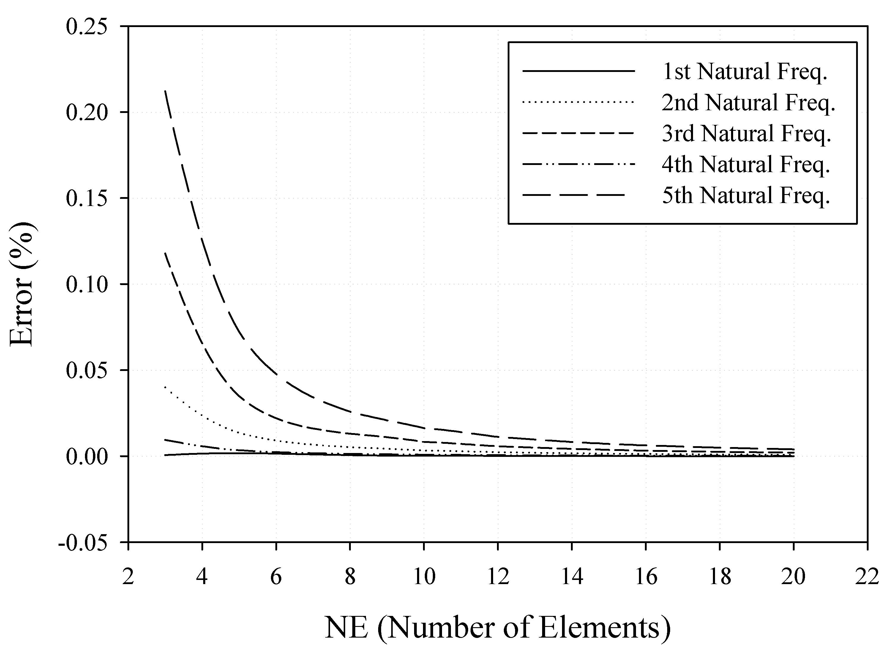
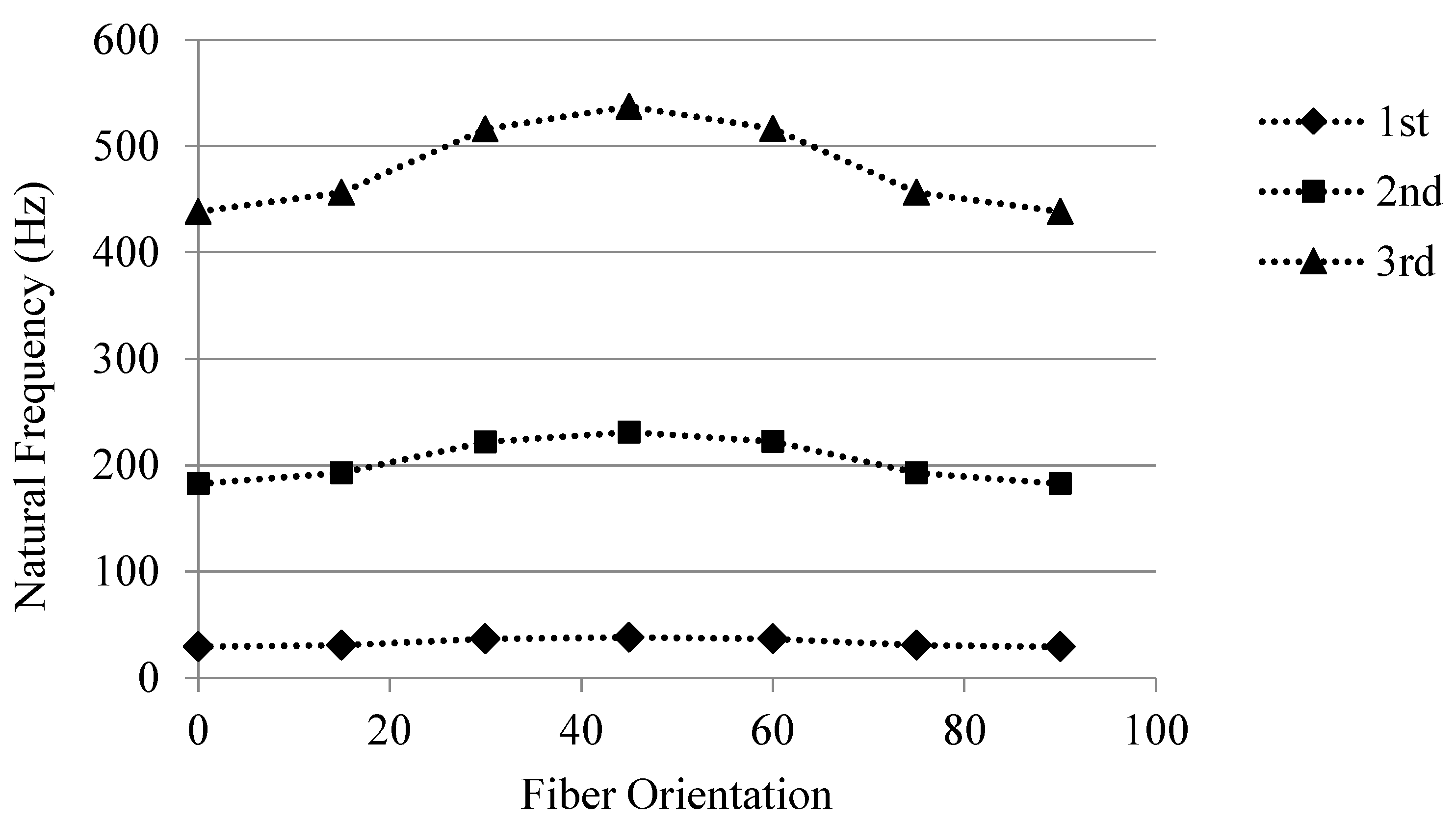
3.1. Single-Layer Glass/Epoxy Composite Beam

Let us first consider a uniform, cantilevered beam composed of glass–epoxy composite material, made up of unidirectional plies with 0.1 mm thickness, with fiber angles in each ply set to +15°, subjected to end moment and axial force. The beam is assumed to be 0.1905 m long and 12.7 mm wide. Based on Banerjee and Williams [10], the beam can be considered equivalent to a single thick ply, with a thickness of 3.18 mm, and the following material and geometric properties derived/considered: bending rigidity, EI = 0.2865 N.m²; torsion rigidity, GJ = 0.1891 N.m²; bending–torsion coupling rigidity, K = 0.1143 N.m²; mass per unit length, m = 0.0544 kg/m; and mass polar moment of inertia per unit length, I_α = 7.77 × 10⁻⁷ kg.m.

A free vibration analysis of the system was performed using the FEM and DFE codes developed in MATLAB, carrying out the assembly of the static (FEM) mass and stiffness and dynamic (DFE) matrices with the application of the system’s boundary conditions and solving the resulting eigenvalue problems. There are no frequency data available in the open literature for such a prestressed composite beam subjected to axial load and end moment. Therefore, both the FEM and DFE codes were first validated for an unstressed composite beam (i.e., M_zz and P were set to zero) as reported by Banerjee and Williams [12], for which exact DSM reference values were available. In the DSM theory, the element frequency-dependent stiffness matrix was developed from the closed form solution to the governing coupled differential equations, and therefore are exact within the limits of the theory. The conventional FEM theory and the corresponding element mass and stiffness matrices, as mentioned in previous sections, were developed based on cubic Hermite and linear interpolation functions for flexural and torsional displacements, respectively. In contrast, the DFE matrices were evaluated using frequency-dependent trigonometric interpolation functions derived using the basis functions presented in Equations (26) and (27).

The unstressed system’s first five natural frequencies evaluated from a five-element mesh modeled using the presented FEM and DFE formulations are presented in

Table 1. Comparison of the first five FEM and DFE natural frequency (Hz) results for M_zz = 0 and P = 0 with the analytical DSM values [12].

Natural Frequency	Exact DSM [12]	5 FEM Elements	5 FEM |Error|%	5 DFE Elements	5 DFE |Error|%	1 DFE Element	DFE |Error|%
1st	30.82	30.82	0.00%	30.82	0.00%	30.82	0.00%
2nd	192.72	192.87	0.08%	192.72	0.00%	192.72	0.00%
3rd	537.38	538.47	0.19%	537.38	0.00%	537.38	0.00%
4th	648.73	648.87	0.02%	648.73	0.00%	648.73	0.00%
5th	1049.73	1053.87	0.39%	1049.73	0.00%	1049.73	0.00%

, along with those obtained using a single-element DFE model and the (exact) DSM data from [12]. As can be seen from Table 1, the FEM frequencies are in very good agreement with the DSM values [12], with a maximum error of less than 0.4% for the fifth frequency, and an average error of less than 0.14%. As expected, the five-element FEM model predicted higher natural frequencies than the DSM values, and the estimated error was found to increase with the mode number, except for the fourth natural frequency. This can be associated with the fact that, in this case, the first, second, third, and fifth modes exhibited bending–torsion material coupling predominated by flexural displacement, whereas the fourth mode was predominantly torsional, i.e., exhibiting the first torsional mode’s behavior. It is worth noting that all the DFE frequencies obtained using both one- and five-element models, in this case, were found to be in perfect agreement with the DSM data, i.e., 0% error. The FEM convergence test results for the unstressed (i.e., M_zz and P were set to zero) beam’s first five natural frequencies are shown in Figure 3.

The bending–torsion coupling behavior in this model is partly caused by the fiber angle and partly by the applied end moment. Depending on the end moment and fiber angle directions, these two coupling sources either intensify or diminish one another’s effects. It is worth noting that in most composite material applications, the resulting couplings between different displacements are undesired. Therefore, knowing the magnitude of the working end moment, the direction of fiber angle and stacking sequence can be tailored in such a way that resulting torsional displacement caused by the material coupling (K) is in the opposite direction of that resulting from the end moment (M_zz), minimizing or, ideally, cancelling the coupling effects.

Once the validity of the FEM and DFE formulations for the unstressed composite beam was established, the vibrations of the prestressed configurations subjected to combined axial load and end moment were investigated. The variation of the uniform, cantilevered composite beam’s fundamental natural frequency versus axial compressive force (obtained from the five-element FEM and DFE models) for M_zz = 20 N.m is shown in Figure 4.

The effect of fiber angle on the vibrational behavior of the composite glass–epoxy beam was also investigated using a five-element DFE model, and the results are represented in Figure 5. As can be seen from Figure 5, at 45°, the fiber angle system exhibited the highest natural frequency, associated with the highest material bending–torsion coupling factor (K_max) at this fiber angle.

A buckling analysis for a single-layer glass–epoxy beam was also carried out using a five-element DFE model, where for each axial force the end moment was varied to find the critical value, M_zzCr, leading to a zero natural frequency (the results are presented in Figure 6). As can be observed from Figure 6, at zero axial force (P = 0), the critical (buckling) end moment was found to be M_zzCr = 48.3 N.m. An increase in the tensile (i.e., positive) axial force increased the critical (buckling) end moment. In contrast, increasing the compressive (i.e., negative) axial forces led to a decrease in critical (buckling) end moment.

Considering the above prestressed, cantilevered composite beam subjected to an end moment of M_zz = 20 N.m and an axial tensile force of P = 10 N, the DFE model was used to extract the system’s first five natural mode shapes (Figure 7 and Figure 8). The natural modes’ flexural and torsional components are separately illustrated in Figure 7 and Figure 8, respectively, showing that the bending was predominant in the first, second, third, and fifth modes of free vibrations, while the fourth was predominantly a torsional mode.

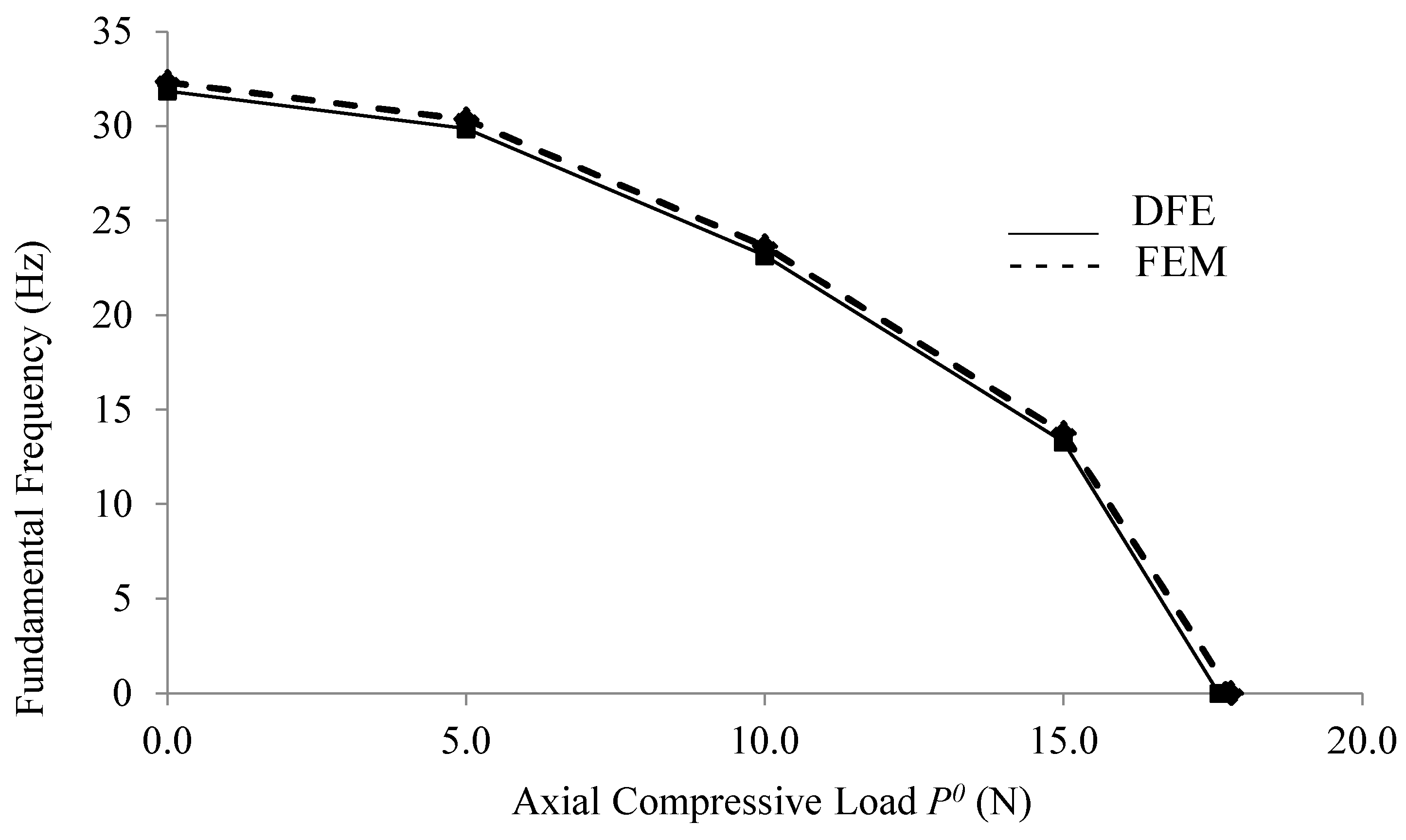
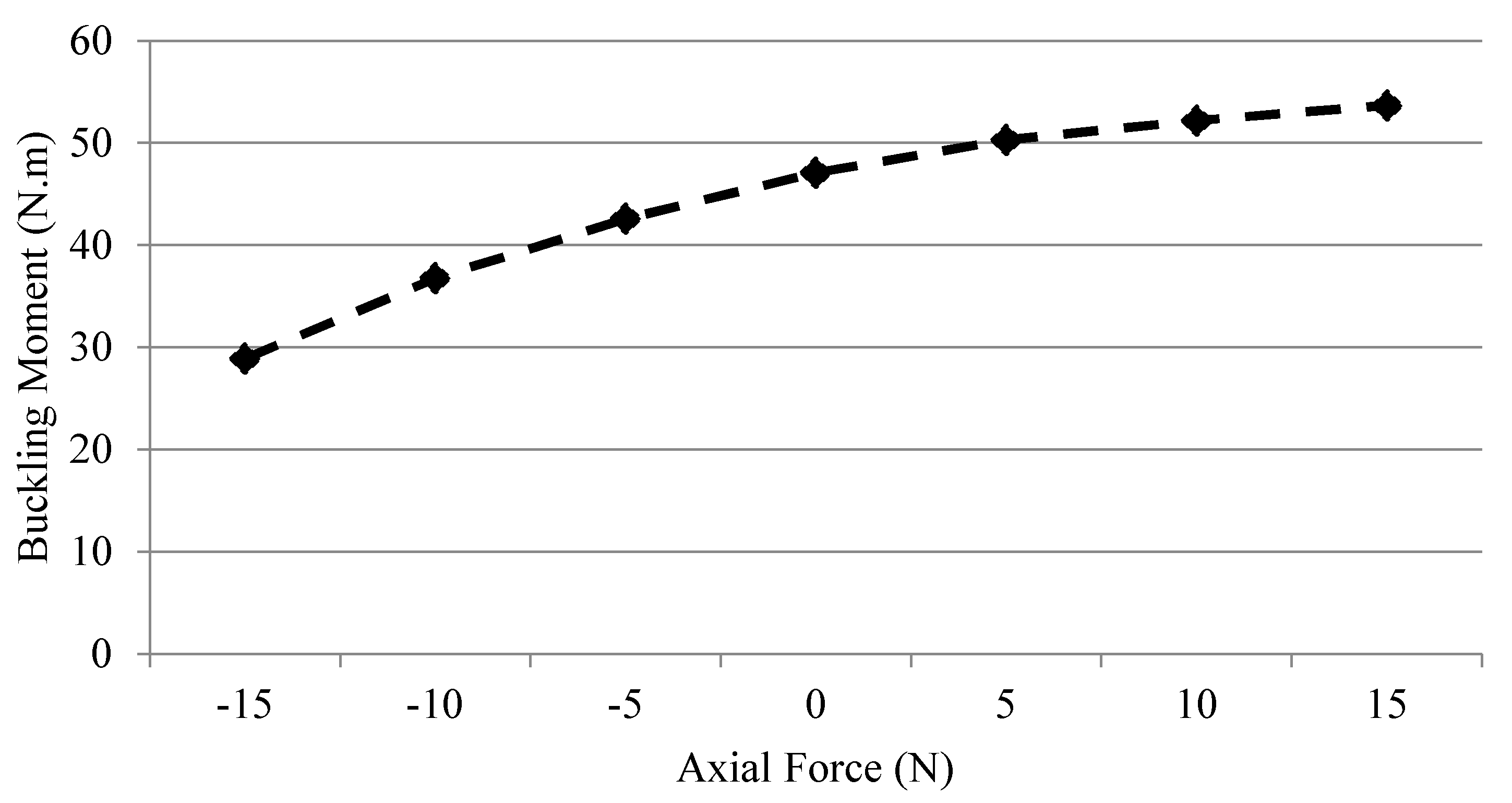
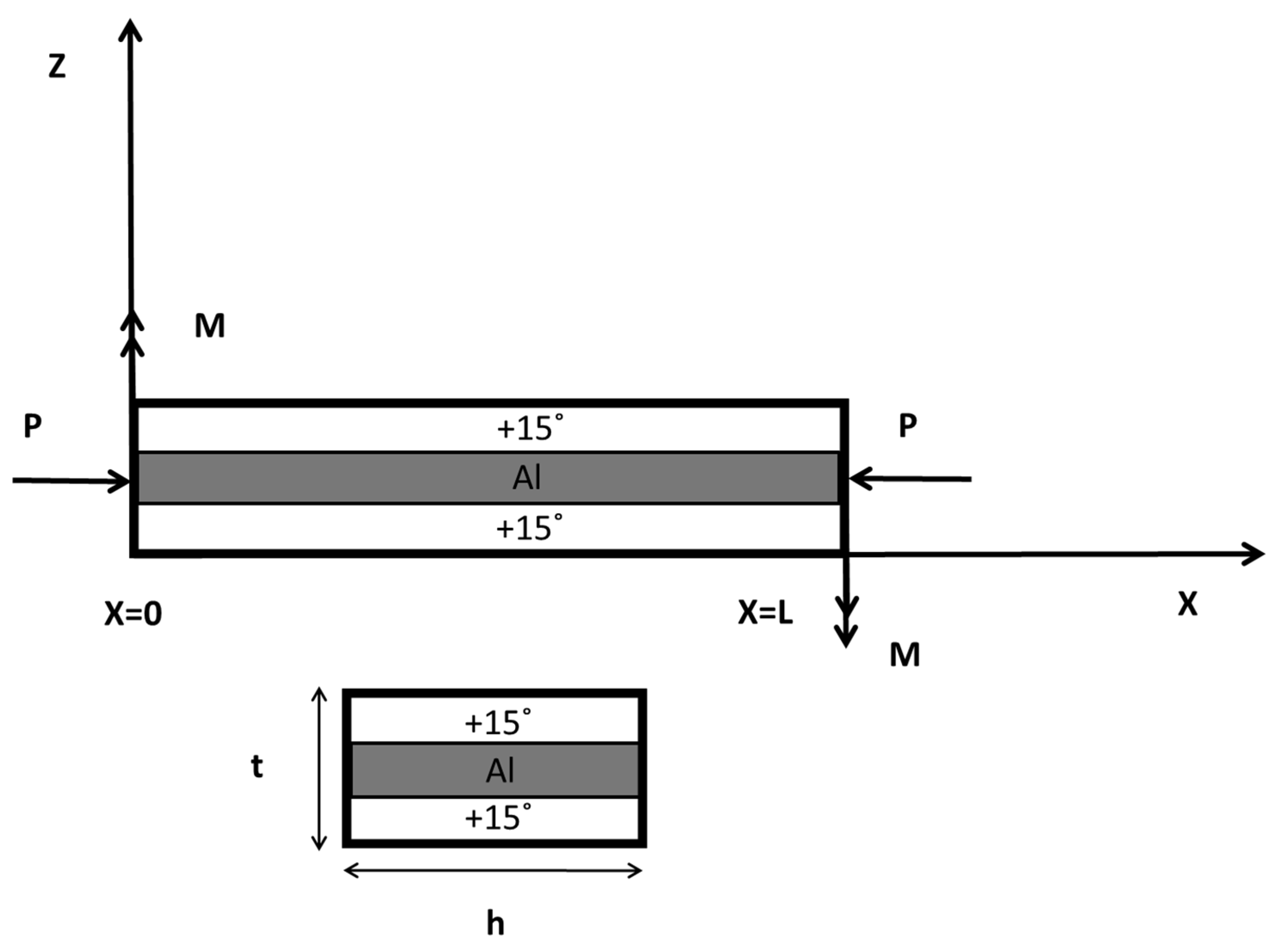
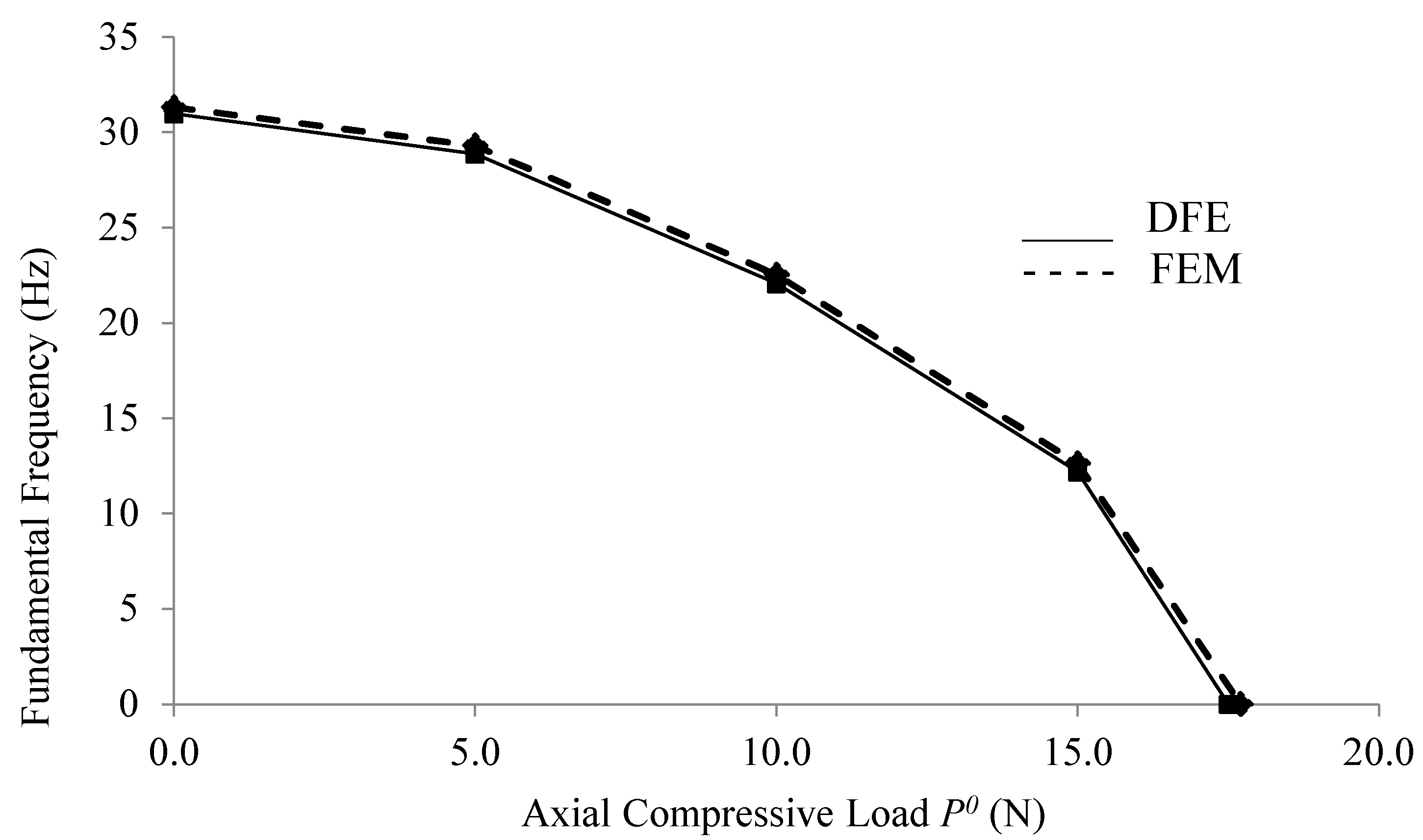
3.2. Three-Layer Fiber-Metal Laminated (FML) Beam

To further investigate the applicability of the presented formulation, the FEM and DFE approaches, together with a simple layer-wise formulation, were used to investigate the free vibrations of an illustrative example of a cantilevered, prestressed, three-layer fiber-metal laminated (FML) beam subjected to axial force and end moment. The FML construction at hand, also known as GLARE (glass-reinforced aluminum laminate), was assumed to consist of two composite face layers, each made of glass–epoxy with +15° fiber angle (as in the previous example), and an aluminum core, as shown in Figure 9.

As with the composite beam in the previous example, this beam had an overall length of L = 0.1905 m, a rectangular cross-sectional area of thickness t = 3.18 mm, and width of w = 12.7 mm. The aluminum core had a mass density of ρ = 2700 kg/m³, shear modulus of G = 26 GPa, and Young’s modulus of E = 70 GPa, and the thickness of all the three layers was considered equal (one-third of the total thickness; t/3). The prestressed FML beam exhibited coupled bending–torsion behavior, partly caused by the fiber angle in the face-layers (leading to the material bending–torsion coupling stiffness, K), and in part by the applied end moment, i.e., geometric coupling. These two couplings, depending on their directions, either alleviate or intensify each other’s effects.

The variation of fundamental natural frequency versus axial compressive force for FEM and DFE, both using five elements with M_zz = 20 N.m, for the FML beam is shown in in Figure 10, and the buckling analysis results are presented in Figure 11. The conventional FEM’s overestimation of the results is once again observed in Figure 10. This is mainly due to the constraints imposed by the polynomial basis/shape functions of the approximation space on the system [3,8,14,15].

4. Discussion

The free, undamped, doubly coupled vibration of a prestressed composite beam subjected to axial force and end moment was modeled using both the FEM and DFE methods, and the results were validated with analytical DSM results. In this modeling, the composite nature of the beam material introduced one (material) coupling term between the bending and torsion displacements in the bending differential equation of motion and introduced one term in the torsion differential equation of motion, while the applied end moment created another (geometric) coupling term in each equation, leading to a total of four coupling terms in the system of differential equations. Because of these coupling terms between the two differential equations, the system had no analytical solution, which led us to use numerical methods for modeling purposes.

The modeling results for the two numerical methods showed that when using same number of elements, the DFE had a higher rate of convergence compared to the FEM method (Table 1). The results also showed that, as expected, for a constant end moment, increasing the compressive axial force decreased the stiffness of the system which, in turn, led to lower natural frequencies (Figure 4). In contrast, increasing the tensile axial force increased the beam’s stiffness and the critical (buckling) end moment (Figure 6). All the vibration modes were coupled and included both torsion and bending components. In the first three modes, bending was dominant, while in the fourth, torsional bending became predominant (Figure 7 and Figure 8). From Table 1, it is inferred that in the absence of an end moment (M_zz = 0) and material coupling (K = 0), a single-element DFE model yields the same results as the DSM method. This can be explained by the fact that in the absence of these coupling terms, the frequency-dependent stiffness matrix in the DFE method (without discretization) results in the same formulation as the DSM analytical solution, as reported in [12].

The effect of ply angle on the vibrational behavior of the composite glass–epoxy beam was also investigated using a five-element DFE model. All of the first three natural frequencies were found to increase from the fiber angles of 0° to +45° and to decrease from +45° to +90° (Figure 5).

Further investigation into the applicability of the presented FEM and DFE formulations to the free vibration analysis of a prestressed, three-layer composite–aluminum sandwich (GLARE) beam showed that this beam had almost the same stiffness and buckling resistance as the laminated composite beam (Figure 4 and Figure 10). Moreover, overprediction of the natural frequencies by the FEM method was once again observed (Figure 10), and it can be justified by constraints on displacements introduced by the polynomial basis and interpolation functions of approximation space in the formulation.

In summary, in both cases studied and presented in this paper, the convergence rates obtained from a frequency-dependent dynamic finite element (DFE) formulation were found to surpass those obtained from the conventional FEM. The DFE’s higher convergence rate is mainly attributed to the usage of the solutions to the uncoupled part of equations as the basis functions of approximation space. In comparison with conventional FEM, which uses simple polynomial shape functions, the interpolation functions derived from these solutions provide much better approximations for element displacements expressed in terms of nodal displacements. This higher convergence rate means that to reach a specific accuracy, DFE requires a much smaller number of elements than FEM. This may not seem like a large advantage in the analysis of simple structures such as the ones studied here, but when it comes to large-scale designs of complex systems, using DFE would lead to much less computation and analysis time.

References

1. Jones, R.M. Mechanics of Composite Materials, 2nd ed.; Taylor and Francis Inc.: London, UK, 1998. [Google Scholar]
2. Berthelot, J.M. Composite Materials Mechanical Behaviour and Structural Analysis; Springer: New York, NY, USA, 1999. [Google Scholar]
3. Hashemi, S.M.; Borneman, S. Doubly-Coupled Vibrations of Nonuniform Composite Wings: A Dynamic Finite Element. Math. Probl. Eng. Aerosp. Sci. 2011, 5, 141–152. [Google Scholar]
4. Abramovich, H.; Livshits, A. Free Vibration of Non-Symmetric Cross-Ply Laminated Composite Beams. J. Sound Vib. 1994, 176, 597–612. [Google Scholar] [CrossRef]
5. Jaehong, L.; Kim, S. Flexural-Torsional Coupled Composite Beams with Channel Sections. Comput. Struct. 2002, 80, 133–144. [Google Scholar]
6. Chen, X.L.; Liu, G.R.; Lim, S.P. An Element Free Galerkin Method for the Free Vibration Analysis of Composite Laminates of Complicated Shape. Compos. Struct. 2003, 59, 279–289. [Google Scholar] [CrossRef]
7. Jung, S.N.; Nagaraj, V.T.; Chopra, I. Refined Structural Dynamics Model for Composite Rotor Blades. AIAA J. 2001, 39, 339–348. [Google Scholar] [CrossRef]
8. Bathe, K.-J. Finite Element Procedures in Engineering Analysis; Prentice Hall: Hoboken, NJ, USA, 1982. [Google Scholar]
9. Kalousek, V. Dynamics in Engineering Structures; Butterworths: London, UK, 1973. [Google Scholar]
10. Banerjee, J.R.; Williams, F.W. Free Vibration of Composite Beams—An Exact Method Using Symbolic Computation. J. Aircr. 1995, 32, 636–642. [Google Scholar] [CrossRef]
11. Wittrick, W.; Williams, F. A General Algorithm for Computing Natural Frequencies of Elastic Structures. Q. J. Mech. Appl. Math. 1971, 24, 263–284. [Google Scholar] [CrossRef]
12. Banerjee, J.R.; Williams, F.W. Exact Dynamic Stiffness Matrix for Composite Timoshenko Beams With Applications. J. Sound Vib. 1996, 194, 573–585. [Google Scholar] [CrossRef]
13. Banerjee, J.R. Free Vibration of Axially Loaded Composite Timoshenko Beams Using the Dynamic Stiffness Matrix Method. Comput. Struct. 1998, 69, 197–208. [Google Scholar] [CrossRef]
14. Hashemi, S.M.; Roach, A. Dynamic Finite Element Analysis of Extensional-Torsional Coupled Vibration in Nonuniform Composite Beams. Appl. Compos. Mater. 2011, 18, 521–538. [Google Scholar] [CrossRef]
15. Kashani, M.; Jayasinghe, S.; Hashemi, S.M. On the Flexural-Torsional Vibration and Stability of Beams Subjected to Axial Load and End Moment. Shock. Vib. 2014, 2014, 153532. [Google Scholar] [CrossRef]
16. Lottati, I. Flutter and Divergence Aeroelastic Characteristics for Composite Forward Swept Cantilevered Wing. J. Aircr. 1985, 22, 1001–1007. [Google Scholar] [CrossRef]
17. Joshi, A. Vibration of Thin-Walled Tubular Structures in the Presence of Static Axial Stress Fields. Ph.D. Thesis, Department of Aeronautical Engineering, Indian Institute of Technology, Bombay, India, 1983. [Google Scholar]
18. Banerjee, J.R.; Su, H.; Jayatunga, C. A dynamic stiffness element for free vibration analysis of composite beams and its application to aircraft wings. Comput. Struct. 2008, 86, 573–579. [Google Scholar] [CrossRef]
Figure 1. Geometry and coordinate system of the model.
Applmech 03 00015 g001
Figure 2. Discretized domain along the beam span using N elements and three DOFs per node.
Applmech 03 00015 g002
Figure 3. FEM error versus the number of elements for the first five natural frequencies. The percent error is relative to the exact values obtained from the DSM [12].
Applmech 03 00015 g003
Figure 4. Variation of the fundamental natural frequency vs. axial compressive force for Mzz = 20 N.m, obtained from the five-element FEM and DFE models.
Applmech 03 00015 g004
Figure 5. Variation of the first three natural frequencies for a composite beam with glass–epoxy composite ply angle using a five-element DFE model with Mzz = 20 N.m and P = 10 N.
Applmech 03 00015 g005
Figure 6. Buckling analysis for a single-layer, glass–epoxy composite, cantilevered beam with a fiber angle of +15° using a five-element DFE model (negative axial force means compression, while positive means tension).
Applmech 03 00015 g006
Figure 7. The bending components for the first five natural mode shapes, obtained using the DFE method (bending displacement is normalized).
Applmech 03 00015 g007
Figure 8. The torsion components for the first five natural mode shapes, obtained using the DFE method (torsion displacement is normalized).
Applmech 03 00015 g008
Figure 9. Three-layer, fiber-metal laminated (FML) beam schematic.
Applmech 03 00015 g009
Figure 10. Variation of the fundamental natural frequency vs. axial compressive force for the cantilevered, three-layer glass–epoxy and aluminum sandwich beam (GLARE), obtained using the five-element DFE and FEM models, with Mzz = 20 N.m.
Applmech 03 00015 g010
Figure 11. Buckling analysis for the cantilevered, three-layer glass–epoxy and aluminum sandwich beam (GLARE), using five-element DFE (negative axial force means compression, while positive means tension).
Applmech 03 00015 g011