Article

Microscale Thermal Modelling of Multifunctional Composite Materials Made from Polymer Electrolyte Coated Carbon Fibres Including Homogenization and Model Reduction Strategies

by
Maximilian Otto Heinrich Schutzeichel
1,*,
Thomas Kletschkowski
1 and
Hans Peter Monner
2,3
1
Department of Automotive and Aeronautical Engineering, Faculty of Engineering and Computer Science, Hamburg University of Applied Sciences, Berliner Tor 9, 20099 Hamburg, Germany
2
German Aerospace Center, Lilienthalplatz 1, 38108 Braunschweig, Germany
3
Faculty of Mechanical Engineering, Institute of Mechanics, Otto von Guericke University Magdeburg, Universitätsplatz 2, 39106 Magdeburg, Germany
*
Author to whom correspondence should be addressed.
Appl. Mech. 2021, 2(4), 739-765; https://doi.org/10.3390/applmech2040043
Submission received: 10 August 2021 / Revised: 24 September 2021 / Accepted: 27 September 2021 / Published: 1 October 2021

Abstract

:
Polymer electrolyte coated carbon fibres embedded in polymeric matrix materials represent a multifunctional material with several application scenarios. Structural batteries, thermal management materials as well as stiffness adaptive composites, made from this material, are exposed to significant joule heat, when electrical energy is transferred via the carbon fibres. This leads to a temperature increase of up to 100 K. The thermal behaviour of this composite material is characterized in this numerical study based on a RVE representation for the first time. Compared to classical fibre reinforced plastics, this material comprises a third material phase, the polymer electrolyte coating, covering each individual fibre. This material has not been evaluated for effective thermal conductivity, specific heat and thermal behaviour on the microscale before. Therefore, boundary conditions, motivated from applications, are applied and joule heating by the carbon fibres is included as heat source by an electro-thermal coupling. The resulting temperature field is discussed towards its effect on the mechanical behaviour of the material. Especially the temperature gradient is pronounced in thickness direction, leading to a temperature drop of 1   ° C mm , which needs to be included in thermal stress analysis in future thermo-mechanically coupled models. Another important emphasis is the identification of suitable homogenization and model reduction strategies in order to reduce the numerical effort spent on the thermal problem. Therefore, traditional analytical homogenization methods as well as a newly proposed “Two-Level Lewis-Nielsen” approach are discussed in comparison to virtually measured effective quantities. This extensive comparison of analytical and numerical methods is original compared to earlier works dealing with PeCCF composites. In addition, the accuracy of the new Two-Level Lewis-Nielsen method is found to fit best compared to classical methods. Finally, a first efficient and accurate 2D representation of the thermal behaviour of the PeCCF composite is shown, which reduces computational cost by up to 97%. This benefit comes with a different Temperature drop prediction in thickness direction of 1.5   ° C mm . In the context of future modelling of multifunctional PeCCF composite materials with multiphysical couplings, this deviation is acceptable with respect to the huge benefit for computational cost.

1. Introduction

A composite material consisting of polymer electrolyte coated carbon fibres (PeCCF) embedded in a polymer matrix is able to provide multiple functions. The typical application of fibre reinforced polymers is lightweight design of load bearing structures. The PeCCF analysed here is able to combine the reinforcement with energy storage in a structural battery [1,2,3], thermal heating in thermal management applications (e.g., de-icing in aircraft structures [4]) and thermo-adaptive stiffness [5,6] which holds perspectives for vibration control. In any case, the objective of the material is to provide multiple functions on system level, which results in advanced weight reduction potential. Special attention is dedicated to the polymer electrolyte coating, which represents an interphase of 500 nm thickness between matrix and carbon fibres in the composite [1,7]. Thereby, the single carbon fibres are electrically insulated against other fibres and against further surrounding material phases. Accordingly, the interphase influences the load transfer between the reinforcement and the matrix [8]. In line with these recognitions, this work analyses the influence of the coating layer on the effective thermal behaviour of the composite in order to identify homogenization strategies for multi-scale material models of this type for the first time.
The multifunctional material is subjected to thermal loads in all application scenarios since it exhibits significant joule heat while electrical energy is transferred in longitudinal direction through the fibres [9]. In case of structural energy storage, additional thermal loads are generated by ion transport in the transversal plane [10]. However, Carlstedt et al. already indicated, that the thermal loads need to be included in the structural design process of structural batteries, where thermal expansion influences stress distributions and effective stiffness of the structure. Until today, the temperature distribution in multiphysics simulation was assumed to be a reference value [11]. With this work, the accurate and fast prediction of temperature distributions inside the PeCCF composite material is emphasised and will highlight the effects of thermal heat flux inside the composite.
Investigations by the authors indicated, that the coating phase can induce a significant stiffness loss in the transversal plane. The polymer electrolyte coating shows thermo-viscoelastic properties, which results in a temperature dependent komplex modulus [6]. Since the coating interphase is important for the load transfer between fibre and matrix, a coating stiffness loss with temperature rise results in an overall effective stiffness loss in the transversal plane [8].
To describe the composite material behaviour on the macroscale (structure or system scale) the thermal behaviour of the compound on the microscale needs to be characterized and suitable homogenization strategies need to be identified. These characteristics could then be part of a multiscale and physically coupled material model, which enables the design of multifunctional lightweight structures. This study presents a numerical characterization of important effects, which are reduced to the unique microstructural architecture and material combination in this composite. Furthermore, traditional homogenization methods as well as a new method for the determination of effective heat conductivity are presented and discussed with respect to the PeCCF composite for the first time. This work contributes to scientific progress with a detailed analysis of influencing factors on the homogenization of the thermal problem and highlights suitable strategies and simplification options to enable computational efficient multiscale models. Furthermore, this study provides new methods for an efficient consideration of the thermal problem in macro-scale simulations of PeCCF composite materials related to structural batteries, thermal management structures and thermo-adaptive stiffness in vibration loaded structures.
Thermal heating and heat conduction are mainly governed by three material properties: heat conductivity ( λ ), specific heat (c) and density ( ρ ). In general, specific heat and density mainly influence the transient heat transfer problem and the heat conductivity governs both, the transient and stationary heat transfer [12]. In most cases composite materials are not exposed to permanent fast temperature changes. Accordingly, the stationary behaviour and thereby the heat conductivity property of composites is the most important characteristic. However, in case of multifunctional applications such as de-icing in aircraft systems, the transient behaviour governed by effective specific heat and effective density of the composite are also of interest. Therefore, both quantities are analysed in this work towards their influence on heat transfer in PeCCF composites.
Research related to heat conduction in composite materials frequently deals with additional influences by thermal resistance on interfaces between material phases [13,14,15,16]. Conclusions towards the influences of interface thermal resistance (also known as Kapista resistance) indicate, that the effect of thermal heat conductivity reduction is especially pronounced for filler materials in the nanoscale ( l 1   nm ). Composite architectures on the microscale do not show such significant influences by interfacial thermal resistance [17,18]. Since carbon fibres’ and the structural polymer electrolyte (SPE) coatings’ dimensions are in the microscale ( l = [ 0.5 , 5 ]   μ m ), this study does not include thermal resistance of interfaces. This general assumption is further supported by physics research, where the main reason for high thermal resistances in composite interfaces is reduced to highly disordered material structures near to the interface and imperfect interface adhesion [15,19]. Kaminski and Ostrowski [20] recently presented a numerical study to analyse the effect of stochastic interface defects on thermal conductivity of a composite material. From numerical experiments they concluded that such defects lead to significant dispersion of the effective thermal conductivity of the composite. However, the SPE coating is believed to offer very good interfacial properties, since the coating procedure is based on directly grafting the coating from a monomer mixture by electropolymerization onto the surface of the carbon fibres, resulting in a pinholefree coating [7]. Furthermore, Kapista resistance is even more pronounced at very low temperatures below 30 K [15,16], which is out of the applied temperature range of such composites ( T a = [ 190 , 475 ] K [9]). Accordingly, results in this work need to be referred to the assumption of negleigible thermal resistance, thus representing an upper boundary for heat transfer on the microscale. In any case, future research needs to focus on an experimental characterization of the composite interface quality.
Filler materials like carbon fibres show intermediate thermal performance where polymer matrix materials offer only poor thermal properties [13,21]. In addition, the architecture of the composite governs the resulting heat transfer behaviour significantly. The longitudinal thermal conductivity is governed by the carbon fibre, beeing arranged in parallel with the matrix material. Fibres and matrix are arranged in series in the transversal plane, where the matrix dominates the heat transfer as single continous material phase. This leads to a significant transversal isotropic thermal behaviour for long fibre reinforced composites [22]. Since the through-thickness (here transversal thickness, compare Figure 1) direction of structures is typically the thermal heat transfer path [12], this study gives special emphasis on this property.
In the PeCCF composite the temperature gradient is present between joule heated fibres and the outer boundary of the composite. Accordingly it is expected, that the transversal thermal heat transfer is not only governed by the matrix, but is even more influenced by the SPE coating layer. With respect to related research, the existance of interphases with reduced heat conductivity typically result in reduced effective heat conductivities [15,23]. The influence of the coating phase in the PeCCF composite on the effective thermal behaviour in thickness direction is highlighted in this work for the first time. Due to the coupling of thermal and mechanical properties of the PeCCF composite, an accurate model for the description of thermal heat transfer is needed, especially in a multiscale approach. Therefore, a suitable method needs to be indicated to homogenize the thermal coefficients (heat conductivity, specific heat and density) of the composite on the microscale. Several approaches, such as the series and parallel method from the rule of mixture (ROM), the Lewis-Nielsen model as well as spatial averaging are known to compute effective properties for two phase composites with cylindrical inclusions (fibres) [22,24,25]. In this work, these models are adopted to the three phase PeCCF composite, with existing modifications of the Lewis-Nielsen model from Kochetov et al. [26] but also with a newly proposed Two-Level Lewis-Nielsen homogenization method.
To evaluate the thermal performance on the microscale in this work, a suitable cubic representative volume element (RVE) with randomly distribted PeCCFs in a polymer matrix is applied in a FEM framework. Generation of the RVE is driven by the aim to comply with periodic thermal boundary conditions. By this approach, discrete as well as homogenized properties can be studied for typical thermal boundary conditions (BCs), such as forced boundary heat flux (Neumann BC), convective heat dissipation (Robin BC) and forced boundary temperatures (Dirichlet BC). Even though the heat conduction performance is independent of boundary conditions, the effects on the desired temperature distribution in the composites are discussed for predefined BCs cases. Based on the mentioned homogenization approaches the accurate thermal field prediction and model reduction techniques for PeCCF composites are discussed for the first time. The related results are important for scientific progress in future models, which account for physically motivated temperature distributions in the material domain coupled with the mechanical behaviour.
The paper is organized as follows: Applied methods for FEM and homogenization modelling are given hereinafter, followed by the presentation and discussion of the results with respect to predefined modelling cases and finished by a summary of the most important conclusions towards thermal characteristics and model reduction techniques for PeCCF composites.

2. Modelling Methods and Material Properties

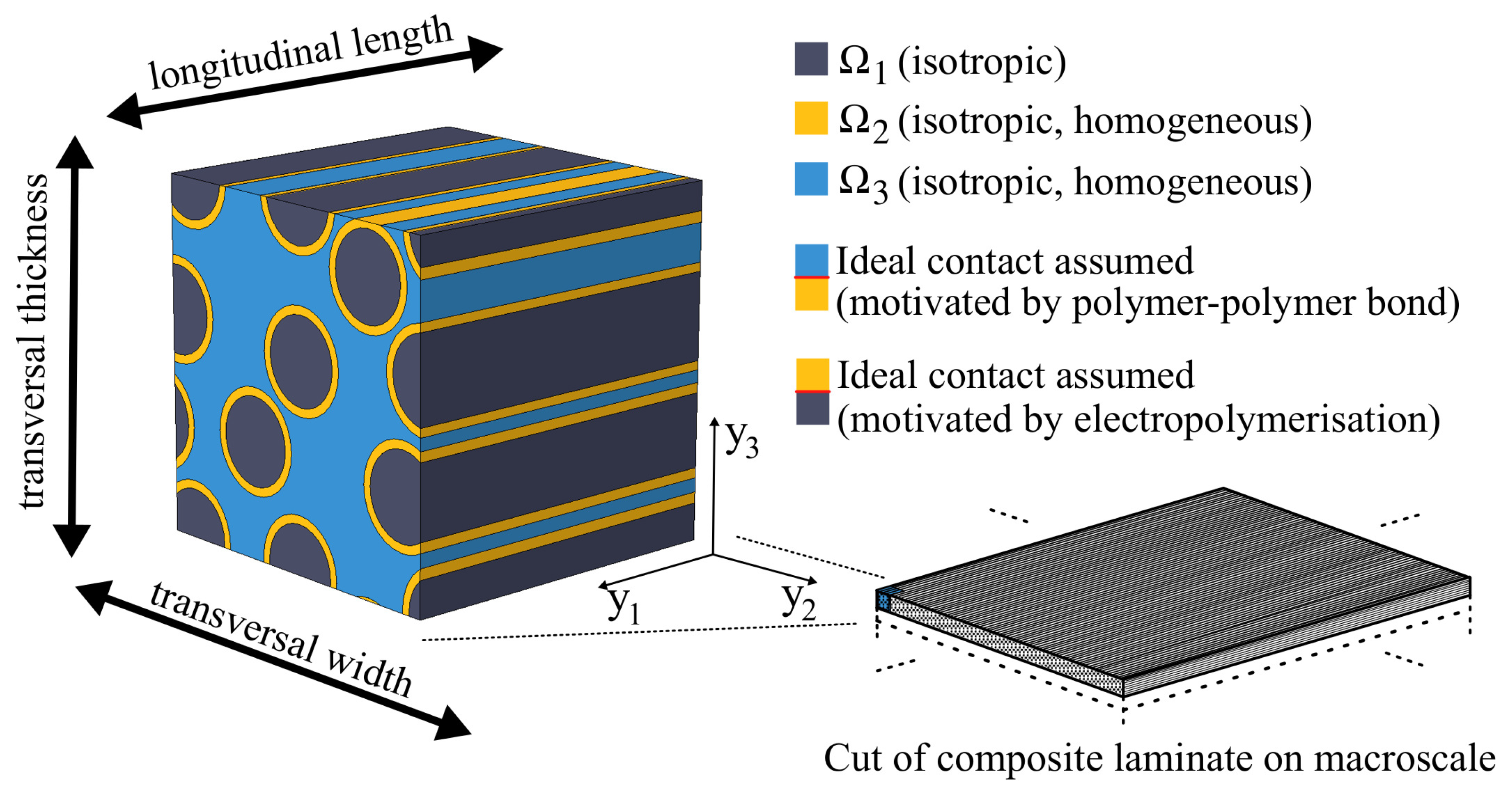
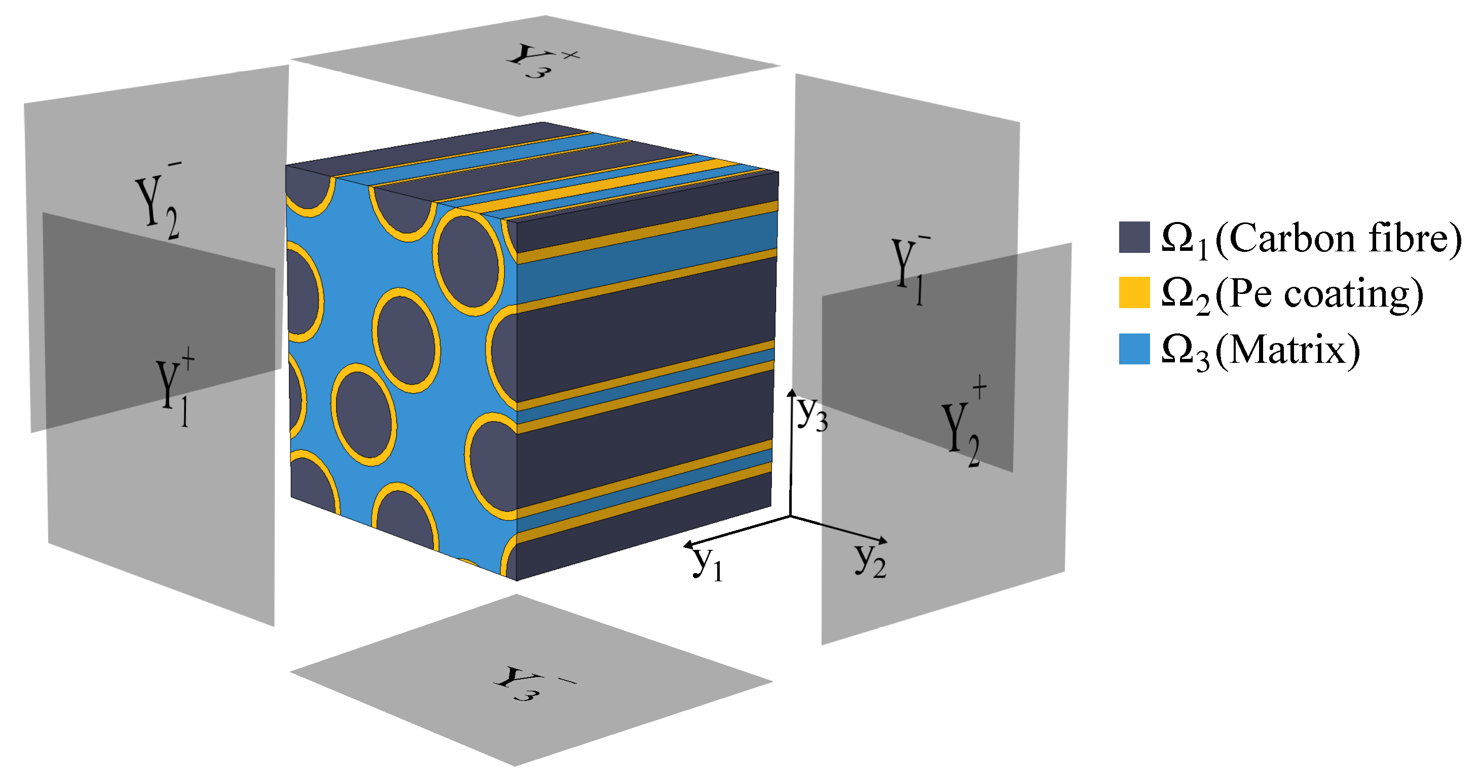
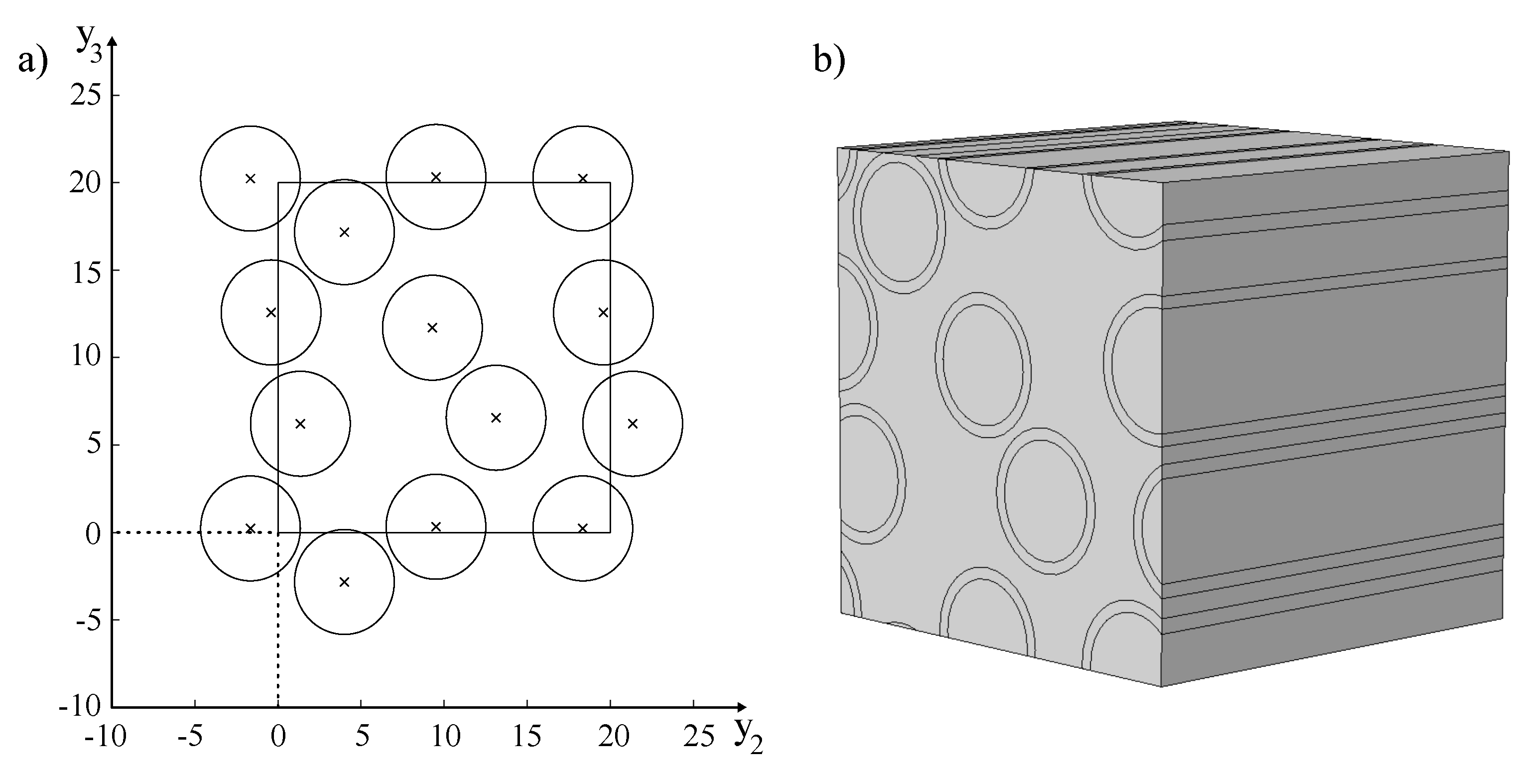
2.1. Representative Volume Element of PeCCF Polymer Composite

The architecture of the material composite is made from polymer electrolyte coated carbon fibres (PeCCFs), which are embedded in a polymer matrix system. The polymer electrolyte coating represents a separate material phase with individual material properties. The combination in an unidirectional reinforced composite material results in transversal isotropic material properties. Foregoing studies from the authors applied cubic unit cells for FEM analysis on this material compound [8], assuming regular distribution of the PeCCFs for mechanical stiffness analysis. The approach in this study is based on randomly distributed unidirectional PeCCFs in an RVE, since, in contrast to mechanical analysis, the single domains contribute differently to the heat flux, depending on its spatial position. Such a spatial differentiation would not be possible in a unit cell. Moreover, the random distibution is believed to represent real composite architectures more accurately, because the long fibre reinforced composite materials show random fibre distributions due to the manufacturing process [27].
The geometry generation is controlled by three parameter (see Table 1) and the desired coated fibre volume ratio v c f . The RVE has a cubic base geometry with edge length a. The diameter of the carbon fibre d f and the thickness of the carbon fibre coating t c are set based on literature data of PeCCFs (references given in Table 1). An algorithm for the generation of fibre positions in the transversal isotropic plane is given in Appendix A.
The resulting fibre positions are then taken for the geometry generation via Matlab LiveLink to Comsol Multiphysics. The RVE consists of a cubic cell (edgelength a) and several cylinders (diameter d f ), which represent the carbon fibres. The coating layer is created by adding cylindric shells of thickness t c and inner radius r c = d f / 2 , positioned along the center points of the fibres. The cylinders and cylindric shells are cut by the faces of the cubic cell. Fibres, which overlap with a cube face, have an associated fibre on the opposite face to assure geometric compatibility after the fibres are cut. This property is important for periodic boundary conditions. Associated fibres are already prepared by the corresponding fibre positions from the algorithm (see Appendix A).
Figure 2 illustrates the sample geometry for discretely resolved calculations in this work with a corresponding fibre volume ratio of v c f = 0.5 . Furthermore, the single material domains are indicated and a suitable global coordinate system is given. Furthermore, the surfaces are named related to the global coordinate system in order to indicate boundary conditions in a formal way in the following chapter.
It should be noted that the fibre volume ratio is defined by the volume of the PeCCFs related to the total volume of the RVE
v c f = n f · ( V f + V c ) a 3
where n f is the number of fibres inside the RVE, V f is the volume of one single fibre and V c is the volume of the coating of one single fibre. Technical data on FEM discretization is given in Appendix B.

2.2. Heat Transfer Problem and Virtual Material Testing

The PeCCF composite shows a thermo-mechanical coupled behaviour, which represents the motivation for this thermal study on the microscale. In thermomechanics theory, a coupling is assumed by a stress function T and a heat flux function q which are in general dependent on the temperature field θ , the temperature gradient θ and the strain field E as independent variables [30]:
T = T ( E , θ , θ ) ,
q = q ( E , θ , θ )
resulting e.g., in the following linear elastic 3D Duhamel-Neumann equation for linearised Cauchy stress T and Fourier’s law for the heat flux vector q :
T = C ( θ ) · E + Δ θ M ,
q = λ · θ
thus being dependent on the temperature and Greens’ linearised strain tensor E , where λ is the vector of anisotropic heat conductivity, Δ indicates a temperature difference, C is a temperature dependent stiffness tetrade and M the coupling tensor of thermal expansion and stiffness of the material. In addition, thermo-viscoelastic materials can show temperature dependent viscosity, which is not analysed here. This coupling between the mechanical and thermal fields higlight the demand for a well understood thermal behaviour of the PeCCF composite material.
The heat flux vector q contributes to the heat transfer equation:
c ρ t θ = q + Q ,
where c represents the specific heat, ρ the density and Q a volumetric heat source. This work intends to calculate discrete solutions of the heat transfer problem on the microscale with an finite element model based on a representative volume element. Such discrete solutions are compared with solutions by a homogenized RVE and an order reduced representative plane element. In this context the most influencing properties of the single material components are highlighted and strategies for model simplification are discussed. With an accurate reduced thermal model (in dimension and in spatial resolution) a future multiscale modelling approach for the thermo-mechanically coupled problem can be computational cost efficient.
The heat transfer problem is resolved on the microscale by the heat transfer equation in each single material phase i of the composite material:
c i ρ i t θ ( x i , t ) = q i + Q i for x i Ω i and , q i = λ i θ ( x i , t ) where i = 1 , 2 , 3
where c i is the specific heat, ρ i the density, λ i the heat conductivity and Q i the volumetric heat source of the related domain Ωi. The symbol θ ( x i , t ) is the temperature in a spatial point of domain Ωi denoted by the vector x i and at time t. For the discrete description the heat conductivity is assumed to be isotropic for all domains and ideal contact at domain interfaces is assumed. For t θ ( x i , t ) = 0 the stationary heat tranfser equation results:
Q i = λ i 2 θ ( x i ) for x i Ω i and i = 1 , 2 , 3
which is only dependent on the heat conductivity and the heat source. This general equation, which applies for each single domain, represents the discrete description of the stationary heat transfer problem on the microscale. The microscale description is applied here to compare solutions from homogenized material properties with the discrete microstructural solution of the thermal heat transfer problem.
Since the material composite analysed here represents a transversal isotropic material, a related description of Fourier’s law in homogenized notation is described
q = λ · θ ( y )
where λ is the homogenized thermal conductivity tensor, θ ( y ) is the temperature gradient vector and q is the homogenized specific heat flux vector. Homogenization techniques are presented in Section 2.4. The global coordinate system for the homogenized case is denoted by y , which is also indicated in Figure 2. With respect to virtual material testing, which applies here for effective heat conductivity computation, Equation (9) can be simplyfied, if the heat flux and temperature gradient are limited to one direction and related to boundary conditions. For a given heat flux in y 1 (longitudinal) direction and adiabatic boundary condition on surfaces Y 2 + , Y 2 , Y 3 + , Y 3 in transversal directions (compare Figure 2), Equation (9) is written as
Q y 1 b c = λ y 1 θ y 1 + θ y 1 a ,
where a , b , c are the dimensions of the control volume (the RVE in our work) and Q is the total heat flux in y 1 direction. Then λ y 1 can be determined and represents the effective heat conductivity in the respective direction. The effective heat conductivities are then included in the effective heat conductivity tensor λ and Equation (8) is rewritten for the homogenized control volume as:
λ θ ( y ) = Q for y Ω .
For the homogenization of composite material properties, several analytical solutions are given in literature, which are frequently based on effective elastic medium theory. The different approaches applied here, are summarized in Section 2.4. All analytical solutions will be analysed in the homogenized thermal heat transfer problem and discussed in Section 3.
For the analysis of the thermal behaviour of the composite material, different boundary conditions, such as prescribed heat flux, convective heat flux, adiabatic condition as well as periodic boundary conditions are applied. Besides a prescribed heat flux, also a physically motivated heat flux, induced by joule heating in current conducting carbon fibres is of interest for the analysis. Therefore a multiphysical coupling to the electrical field is included in our study. In order to simplify the results interpretation, two different sets of boundary conditions are distinguished hereinafter:
  • Case 1: Virtual thermal conductivity measurement
For the virtual measurement of the effective heat conductivity in the transversal plane of a RVE, periodic boundary conditions are set to the RVE boundaries Y 1 + , Y 1 and Y 2 + , Y 2 (compare [24], see Figure 2):
Δ θ ( Y 1 + ) Δ θ ( Y 1 ) = Δ θ y 1 0 = 0
Δ θ ( Y 2 + ) Δ θ ( Y 2 ) = Δ θ y 2 0 = 0
To enforce a temperature distribution in the RVE in y 3 direction, one boundary is set to a suitable reference temperature θ r and one boundary is set to an inward heat flux q 1 (compare Figure 2)
θ ( Y 3 + ) = θ r
q ( Y 3 ) = y 3 · q 1 .
It should be noted, that the resulting inward heat flux q ( Y 3 ) is defined to be a positive heat flux, where y 3 is the unit vector of y 3 direction. With the resulting temperature difference θ y 1 + θ y 1 Equation (10) can be solved for λ and an effective, virtually measured, heat conductivity can be computed. These boundary conditions can also be altered to study heat conductivities in other directions [24].
  • Case 2: Joule heating and heat transfer
In order to study the temperature distribution in the RVE with respect to joule heating, another set of boundary conditions is given for case 2. Since joule heating induced by the carbon fibres is the usual scenario in multifunctional applications, this case is modelled here in order to understand the influences of homogenization on the resulting temperature field. Therefore, periodic boundary conditions are set to the RVE boundaries Y 1 + , Y 1 and Y 2 + , Y 2 again (compare case 1, Equations (12) and (13)). In y 3 direction an adiabatic condition is set to surface Y 3 and a convective heat dissipation condition is set to surface Y 3 + :
q ( Y 3 + ) = y 3 · h · A · ( θ θ a )
q ( Y 3 ) = y 3 · q 1 with q 1 = 0 .
Heat dissipation is modelled by Robins’ boundary condition, which assumes the temperature difference of ambient temperature θ a (outside the RVE) and the temperature inside the RVE θ to be proportional to the heat flux with a convective heat transfer coefficient h and the convective surface area A (see Equation (16)). It should be noted, that this is a special case, where the RVE is assumed to have an interface with the environment. Nevertheless, this assumption is relevant to understand effects which result from heat generation inside the carbon fibre domain Ω 1 by joule heat and heat transfer from the composite to the environment. This is most important for interpretations towards temperature distributions in thickness direction ( y 3 ), which will be an important characteristic in future multiscale models and is therefore focussed in this study.
Joule heating in the carbon fibre domain is introduced by
Q p = J · Ξ = κ | J 2 | , with
J = j · y 1
where J is the vector of the electric current density, which is given by a constant electrical current density j and the inward surface normal y 3 at surface Y 1 . In this case, the electrical current is applied in longitudinal direction y 1 in domain Ω 1 . The symbol Ξ is the electric field vector and κ is the specific electrical resistance. Q p represents the joule heating power per unit volume. Accordingly, the carbon fibre is the only material which acts as thermal heat source related to joule heating. The other materials are assumed to be electrical insulating which means, that κ is assumed for domains Ω 2 and Ω 3 (compare Figure 2). In order to enable the electrical current flow, a electrical ground condition is applied:
U ( Y 1 + ) = 0 V ,
where U represents the voltage. With respect to the applied inward electrical current density (Equation (19)) an electrical potential in domain Ω 1 is predefined. The technical implementation in Comsol Multiphysics is described in Appendix B.

2.3. Assumptions and Material Properties

The analysed material composite consists of three material phases (compare Section 2.1) with individual material properties. Table 2 summarizes all applied material properties, which are needed for discrete solutions based on the RVE model, as well as for homogenized effective properties based on analytical models (see Section 2.4).
The carbon fibre type IMS65 reffered to for domain Ω 1 is chosen, since it has been foussed in structural battery and multifunctional composite research in the past decade [1,2,7,9,33]. In general, also other fibre types could be suitbale for multifunctional applications. However, the carbon fibre is assumed to be thermodynamically isotropic (see Figure 1), which means that thermal conductivity λ 1 and specific heat c 1 are independent of directions. Basically, this assumption is uncommon, since literature frequently reports transversal isotropic thermal conductivity of carbon fibres [21]. However, it is expected that this impact is negligible compared to other effects, since the thermal conductivity of the coating and the matrix material are much smaller and thereby, dominate the heat conduction. This supports the assumption of isotropic material properties in domain Ω 1 . However, this assumption is discussed based on results for homogenized heat cunductivity in Section 3.
The coating material (domain Ω 2 ) is originally made by electropolymerisation of a monomer mixture containing methoxy polyethylene glycol (350) monomethacrylate (SR550) and tetraethylene glycol dimethacrylate(SR209). Both monomers are included with a ratio of 1:1 by weight. The mixture is enriched by 8% lithium trifluoromethanesulfonate (Li-triflate) and dissolved in dimethylformamid (DMF) [8]. The resulting coating was identified to be promising as structural polymer electrolyte (SPE) coating [1,7]. This special coating material is interesting for structural battery applications as well as for further multifunctional applications, which was investigated by several authors [1,2,4,7,8,9,33,34]. To follow up with our new study, this coating material was cept, although other SPE coatings are reported in literature [6,35,36].
The matrix material (domain Ω 3 ) is assumed to be an epoxy polymer. Although energy storage applications demand for further constituents in the surrounding matrix, this simplification is done to ease interpretations on thermal behaviour with respect to joule heating carbon fibres. The matrix Ω 3 as well as the coating phase Ω 2 are assumed to be homogeneous polymer materials and therefore to be isotropic [32] (see Figure 1).
For all domains, temperature invariant properties (density ρ , specific heat c, heat conductivity λ ) are assumed and alle given properties in Table 2 refer to room temperature. Changes in thermal properties are often indicated at very high temperatures θ > 800 K [31]. In our study, the temperature interval is limited by θ max < 573 K which is the upper limit where the coating material is degenerated and θ min > 223 , 15 K which is the lower limit e.g., in airframe applications [9]. In addition, the electrical conductivity of the carbon fibre (domain = Ω 1 ) is assumed to be constant, which was found experimentally in earlier works by the authors [9].
In addition, thermal resistance (Kapista resistance) at interfaces of domains Ω 1 , Ω 2 and Ω 3 is neglected in this study (see Figure 1). As already indicated in the introduction (see Section 1) thermal resistances at domain interfaces of composite materials are typically induced by interface defects and are commonly relevant on the nanoscale l 1 nm only (see [15,17,18,19]). The electropolymerization process leads to a dense and pinhole free coating of the carbon fibres [7,9], giving reliability to the assumption of negligible thermal resistance between Ω 1 Ω 2 . The coated carbon fibres are embedded further in liquid epoxy resin material and usually cured by vacuum assisted methods, which avoids air inclusions between Ω 2 Ω 3 . Furthermore, research on carbon fibre to matrix interface quality highlighted, that interphases like the PeCCF coating improve the matrix bonding quality (see e.g., [37]). However, this special composition of PeCCF coating and epoxy matrix is not examined in terms of interface quality yet and should be part of future scientific work in terms of verification. The presented material properties and assumptions serve as input for FEM and analytical homogenization methods presented hereinafter.

2.4. Homogenization Methods

This chapter summarizes general methods for homogenization of material properties. The effect of these methods on thermal heat transfer is discussed within the results section of this work.

2.4.1. Spatial Averaging

Spatial averaging is a common homogenization method. Since the goemetry and thereby the single domains are defined by the RVE, the desired quantity can be homogenized by the volume average
k = 1 V V k i d V with k i Ω i ,
where k is the homogenized material property and k i is the quantity of the single domain Ω i . Related to the three-phase system the analytical solution reads
k = 1 V ( k f V f + k c V c + k m V m ) ,
where V i are the single total volumes of each material phase. This homogenization method includes the assumption that all material domains contribute independent of directions or geometrical properties to the homogenized quantity. Accordingly, the result is a volume weighted average of the material properties k i . This is typically similar to a parallel connection of domains, which is only the case for the y 1 direction here (see Section 2.4.2, compare Voigt’s solution for volume averaged strain [38]).
This method is applied in Comsol Multiphysics (v5.5) via the “volume average” function under “derived values” in the results analysis section. Thereby the model accounts for the present mesh and material domains (see Figure 1 and Appendix B).

2.4.2. Series and Parallel Connection

The classical series and parallel model assume that the properties act in a direction dependent manner with respect to their volume fraction. A suitable example in the present microstructure is the thermal conductivity, which is arranged in parallel along the y 1 axis and in series in the transversal plane ( x 1 x 2 ). This assumption is known from the rule of mixtures, which is typically applied in structural mechanics to estimate effective stiffnesses. In general, the equations related to the rule of mixture read
k y 1 = v f · k f + v c · k c + v m · k m ,
k y 2 = k y 3 = v f k f + v c k c + v m k m 1 ,
where k indicates the homogenized material quantity with respect to the global directions (index), v indicates the volume fraction of the domain and indices represent the material (f—carbon fibre, c—coating, m—matrix material) [38]. These two cases are furthermore known as the upper and lower bound for the homogenized quantity. In many cases, the resulting effective quantity is found between these bounds [38]. The rule of mixture does not include any geometrical information about the composite micro architecture, which can lead to significant deviations from effective properties in the transversal plane of a composite.

2.4.3. Three-Phase Lewis-Nielsen Model

Kochetov et al. [22] proposed a new three phase approach for the determination of the effective thermal conductivity of a composite with three individual domains. This approach is based on the classical Lewis-Nielsen equations for the elastic modulus of a two-phase composite, which where derived based on the Kerner equations (see also [39]):
M M 1 = 1 + A B ϕ 2 1 B ϕ 2 with
B = ( M 2 M 1 ) 1 M 2 M 1 + A
where M, M 1 and M 2 represent the moduli of the composite, material phase 1 and material phase 2 respectively. Parameter A includes geometry and Poisson’s ratio of the filler phase, parameter B includes the relation of the moduli of both material phases and ϕ 2 is the volume ratio of the filler material. In [39] these basic equations are developed towards the following set, which is applied by Kochetov et al. [22]:
k y 2 , y 3 = k m 1 + ξ η v c f 1 Φ η v c f with
η = k c f k m k c f + ξ k m ,
Φ = 1 + ( 1 v c f , max ) v c f , max 2 v c f and
ξ = 2 l d .
In this set of equations, ξ represents a shape factor for different filler types [25], which depends on the length l and the diameter d of the PeCCF. The parameter η (B in Equations (25) and (26)) is a function of the homogenized property in the single domains including the shape factor ξ (A in Equations (25) and (26)) and Φ is a function of the volume fractions. Compared to Kerners Equation (25) the function Φ was introduced here to improve the results (see [40]), by taking the maximum filler volume into account. The maximum filler volume fraction is denoted by v c f , max . The index cf indicates the properties of the PeCCF. Kochetov et al. [22] inlcuded the third phase by adding a rule for the coated particle (in this case the coated carbon fibre), which is done by the series connection of the ROM
k c f = v p f k f + v p c k c 1 ,
where v p f and v p c represent the particle related volume fractions of fibre and coating domain respectively. The approach of the Lewis-Nielsen model was originally derived for randomly oriented fibres, where a direction independent homogenized quantity was expected. In this case, the Three-Phase Lewis-Nielsen model is only applicable for the transversal plane ( y 2 y 3 ), as the model is related to a series connection of material properties [25].

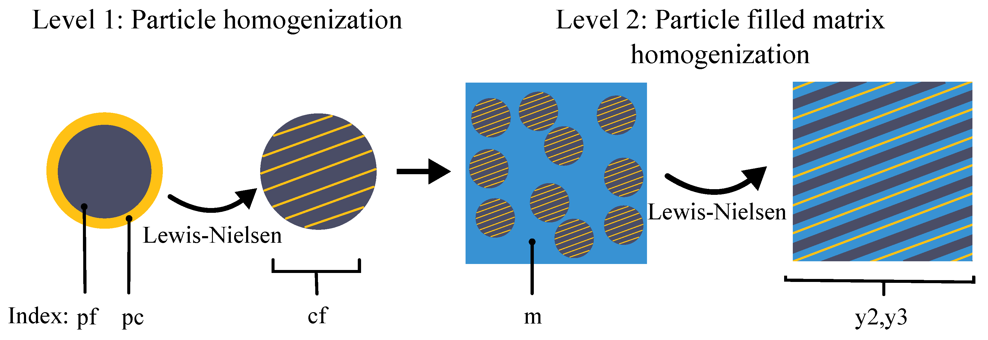
2.4.4. New Two-Level Lewis-Nielsen Approach

During investigations towards thermal conductivity homogenization, the presented classic approaches (Section 2.4.1, Section 2.4.2 and Section 2.4.3) did not meet the desired accuracy (see Section 3). A significant improvement was achived by combining the Lewis-Nielsen method not only based on the coated fibre as filler but also on the filler particle level. Accordingly, Equation (31) is replaced by the Lewis-Nielsen equations:
k c f = k p c 1 + ξ η v p f 1 Φ η v p f with
η = k p f k p c k p f + ξ k p c ,
Φ = 1 + ( 1 v p f , max ) v p f , max 2 v p f
where the single properties are related to the carbon fibre-coating compound. Figure 3 presents the property indices of the Two-Level approach related to the material phases and respective level of calculation. Similar to Equation (31), the result of Equation (32) is applied to the Lewis Nielsen approach for level 2 (Equations (27)–(30)).
The volume ratios for the single calculations in level 1 and 2 are given in Table 3. To the knowledge of the authors, this approach is new to the extend, that the Lewis-Nielsen equations are applied to the two-phase particle (PeCCF) and to the composite made from the coated fibre (cf) and a matrix (m) system. This approach is called “Two-Level Lewis-Nielsen” model hereinafter. The applied parameter are given together with results from this approach (see Section 3.1).

2.5. Principles for Model Reduction

In addition to the material homogenization, the RVE model can be further reduced with a 2D approach, neglecting the heat flux in y 2 direction ( q y 2 = 0 ). This assumption is valid with respect to typical laminates (compare Figure 1) where the temperature distribution in y 1 y 3 parallel planes is expected to be equal. This condition is similar to an adiabatic boundary condition on surfaces Y 2 , Y 2 + in transversal width direction.
This reduction to a 2D planar approach has influences on the general equations, governing Joule heating and heat transfer. Hereinafter, Equations (6), (8) and (18) are rewritten in a 2D approach:
d a c ρ t θ ( y i , t ) = d a λ 2 θ ( y i , t ) + Q
Q = d a λ 2 θ ( y i )
Q p = d e q κ | J 2 |
where d a is the equivalent thickness of the composite material, d e q is the equivalent thickness of the joule heating material (carbon fibres) in y 2 direction and triangular brackets indicate homogenized properties. The homogenized properties are case dependent calculated from equations in Section 2.4. The index i indicates the two directions in the 2D case, where i = 1 , 3 . The parameter κ is defined to be the carbon fibres’ specific resistance, since it is the related joule heating material.
For all calculations in this study, the following assumptions, referring to the out of plane thickness, are made:
d a = a ,
d e q = v f · a 3 a 2 = v f · a ,
where a is the edge length of the RVE (3D). The equivalent thickness d e q is derived from the joule heating domain, which is the total of the carbon fibres within the RVE. The effect of joule heating is proportional to the volume of the joule heating material, which is the carbon fibre domain Ω 1 only. Accordingly the volume of carbon fibres needs to be represented by this definition of the equivalent thickness d e q . The effective RVE volume is represented by the constant d a = a related to the heat Equation (35).
The boundary conditions are identical to those defined in Section 2.2. Former surfaces are now represented by the edges of the 2D square domain multiplied by the respective out-of-plane thickness d a . Since direction y 2 is neglected in this 2D approach, the thermal heat exchange on surfaces Y 2 + and Y 2 is neglected and can be understood as adiabatic condition. Due to the homogeneous properties of the composite in y 2 direction mentioned above, the assumption of a negligible heat flux in y 2 direction is plausible.

3. Results and Discussion

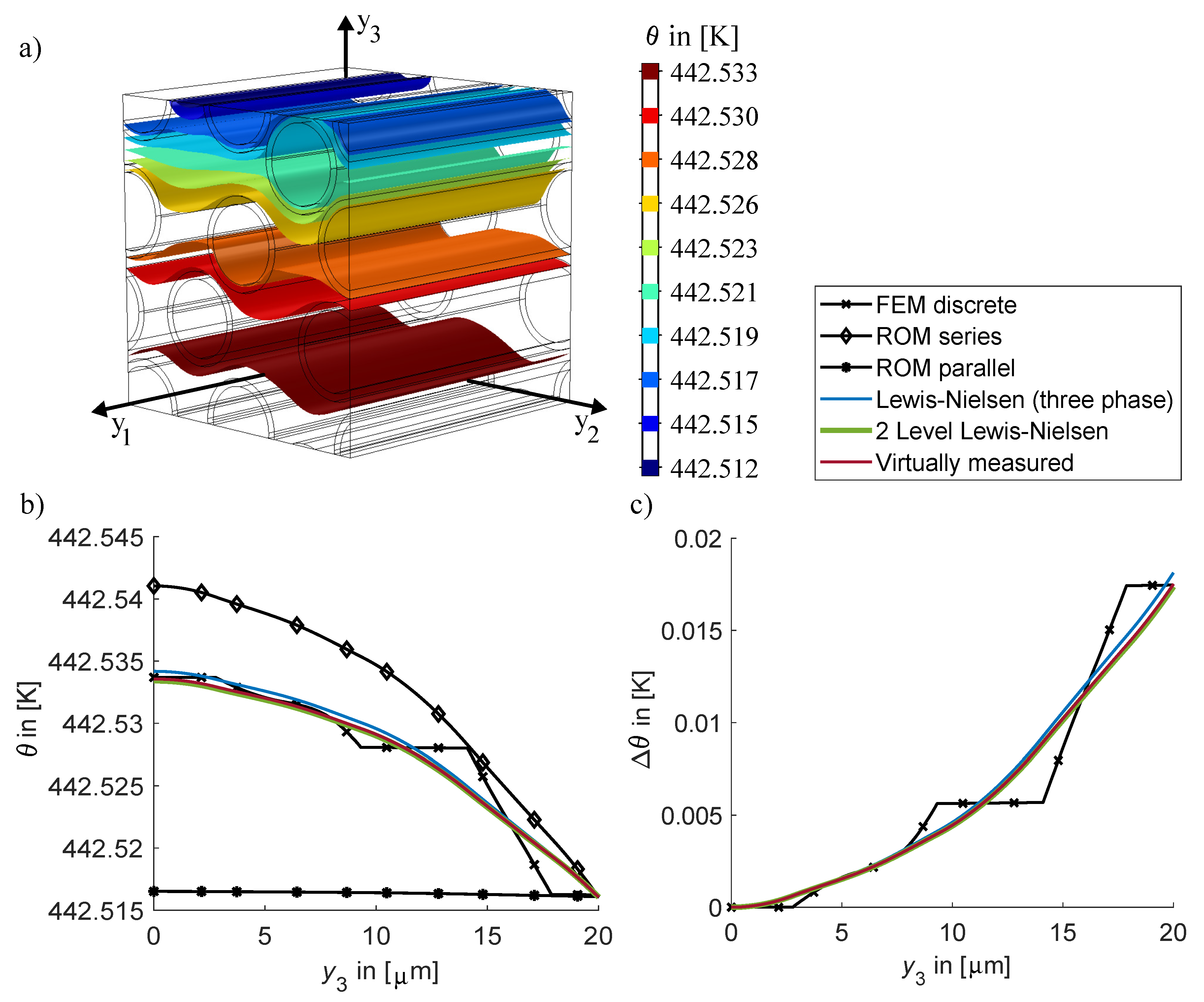
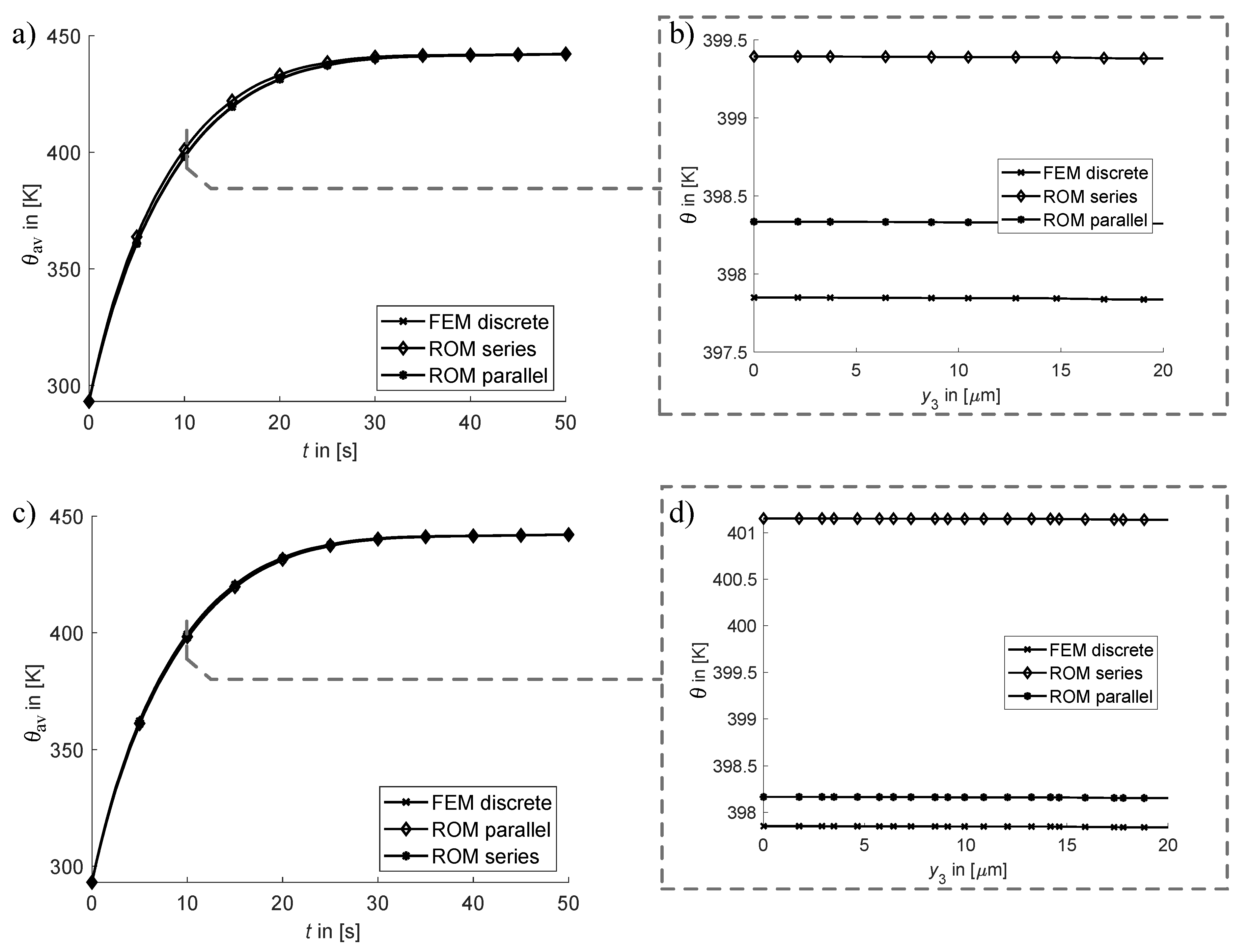
3.1. Stationary Heat Flux Solution and Accuracy of Homogenization

The described methods for homogenization (see Section 2.4) are applied to calculate effective thermal conductivities for the composite material. Table 4 presents the calculated effective thermal conductivities and the respective parameters contributing to the result from analytical equations. In addition, the virtually measured thermal conductivity vector of the RVE is included, to compare the analytical solutions with direction dependent measures. The results presented here are directly related to the different homogenization methods presented in Section 2.4. These results have an important effect on the accuracy of the temperature distribution prediction (see Figure 4). Table 3 completes the applied volume ratios.
The rule of mixtures (ROM) results in upper and lower bounds for the effective thermal conductivity. The upper bound is associated with the parallel case, which is related to the longitudinal direction ( y 1 ), where the single domains are aligned in parallel. The result is identical to the volume average from the RVE finite element model and to the virtual measurment in y 1 direction (compare bc case 1, Section 2.3). Accordingly, this quantity is found to be well defined with negligible variance. The lower bound is represented by the series case of the ROM, which is typically associated with the transversal plane ( y 2 , y 3 ). The results from the Three-Phase Lewis-Nielsen method and the new Two-Level Lewis-Nielsen method appear in between these bounds. Compared to the virtually measured effective thermal conductivities in the transversal plane ( λ 2 , λ 3 ), the Three-Phase Lewis Nielsen model and the Two-Level Lewis-Nielsen model represent more suitable bounds for the effective thermal conductivity in the transversal plane. It should be noted that the Parameter A p f in the Two-Level Lewis-Nielsen model represents the small influence of the coating domain on the thermal conductivity of the coated carbon fibre in transversal direction. In the Three-Phase Lewis-Nielsen model, the effect of the polymer electrolyte coating is overestimated. However, these narrow bounds suit very well to the quantities identified by the virtual measurement, which exhibit a certain influence by the discrete geometric PeCCF distribution in the transversal plane. Comparing the numbers in Table 4 highlights that both methods enable the estimation of the natural dispersion of local thermal conductivities in PeCCF composites with random fibre distributions. This is confirmed by the following plots of resulting temperature distributions.
With respect to this recognition, the analytical models of the Three-Phase Lewis-Nielsen method and the new Two-Level Lewis-Nielsen model are expected to represent accurate effective thermal conductivities for the calculation of the effective thermal heat problem in the transversal plane.
This is proved by analysing the resulting temperature distribution for boundary conditions case 2 (compare Section Figure 2). The following conditions are applied:
j = 2.73 · 10 6 A m 2 ,
U ( Y 1 ) = 0 V ,
θ 0 = θ a = 293.15 K ,
h = 5 W m 2 · K .
These conditions are set for all calculations referring to boundary conditions case 2, where θ 0 represents the starting temperature for the solution of the heat transfer problem and U ( Y 1 ) is the ground condition for the electro-dynamic problem. The convective heat coefficient is assumed based on literature, where this is a typical number for heat convection between solid surfaces and air [12]. It should be noted, that especially this coefficient is sensitive to environmental conditions, material and geometry. Accordingly, this boundary condition needs to be understood as an idealized situation.
The stationary heat transfer problem is calculated based on these settings and special emphasis is on the temperature distribution in thickness direction (see Figure 1). This focus is motivated by the fact that the laminate is typically designed as a plane or curved but thin structure, which dissipates heat to the surrounding environment. The simple but accurate prediction of the temperature distribution in the thickness direction is crucial for inlcuding thermo-mechanical stresses and strains as well as temperature dependent stiffness of the composite in future multiscale models.
Figure 4a shows the resulting isotherms across the RVE with respect to the discrete FEM solution. It is indicated that the isotherms don’t appear as parallel planes which indicates the influence of the joule heating carbon fibres. Accordingly, the temperature distribution is directly influenced by the carbon fibre distribution. The distance between the isotherms decreases towards the upper surface, which indicates that the temperature gradient is increased near to the heat convecting surface. A more detailed insight is enabled by Figure 4b,c. In Figure 4b, the temperature is plotted against the y 3 axis, where ( y 1 , y 2 ) = ( 10 μ m , 10 μ m ) are set and the different solutions for discrete and homogenized heat conductivities from Table 4 are distinguished. Starting with the FEM discrete profile, the increase in temperature gradient along the y 3 axis is clearly indicated. However, along the carbon fibre domain a nearly constant heating temperature is found, which is explained by the 50 times higher thermal conductivity of the carbon fibre compared to the matrix material. Furthermore, the small thermal conductivity of the coating and matrix materials lead to a large negative temperature gradient, especially for material points far from the surface ( 0 μ m y 1 10 μ m ). Since the coating material represents an additional third material phase compared to classical fibre reinforced materials, its significant effect on the temperature gradient in the transversal plane is highlighted. The distance between PeCCF should be minimized by high fibre volume ratios in order to minimize the temperature gradient. This is especially required, since the coating layer limits the fibre volume ratio geometrically by its constant thickness layer around each single fibre.
Furthermore, the single effective heat conductivities are applied and the resulting temperature distribution is given in Figure 4b. The ROM results appear as upper and lower bound. The virtually measured thermal conductivity fits best to the FEM discrete curve as an average. The Three-Phase Lewis-Nielsen approach from Kochetov et al. [26] overestimates the reducing effect of the coating on the effective thermal conductivity of the PeCCF. This can be explained by the fact, that the ROM series method is used for the coated particle. The overestimate is adjusted by applying the Lewis-Nielsen approach also for the coated particle, as explained in Section 2.4.4 for the new Two-Level Lewis-Nielsen method. This enables the accurate calculation of the effective thermal conductivity of the PeCCF composite by analytical equations of the Two-Level Lewis-Nielsen method. Accordingly, the application of a virtual measurement can be omitted and the result from the Two-Level Lewis-Nielsen method can be applied to homogenize the composite materials’ thermal conductivity. This is an efficient simplification for the prediction of the temperature distribution in the composite and helps at increasing the efficiency of future coupled stationary multiscale calculations including the heat flux problem.
Another important effect with respect to composite mechanics is highlighted in Figure 4c. Here the Temperature difference
Δ θ = θ ( y 3 ) θ max ( y 3 ) ,
is shown versus the thickness direction y 3 . Related to the thickness of a = 20 μ m a temperature gradient of Δ θ = 1 · 10 3 K μ m is indicated. With respect to the macroscale of a laminate being several mm thick, the temperature change will be at least Δ θ = 1 K mm . This number is a minimum average, since the non-linear slope of the temperature distribution will increase the discrete temperature gradient. This is important for thermo-mechanical couplings in multiphysics models of the composite, where the stiffness is directly coupled to temperature. The indicated temperature gradient will be important for inter-laminar thermal stress states, which can increase the risk for failure of the material by combined multiphysical loads.
With respect to a possible application scenario as a thermal management material (e.g., for de-icing in aircraft structures), the indicated temperature loss across the thickness-direction can be neglected. The overall temperature level of θ > 400 K (see Figure 4) is promising for the heating purpose. Summarising, the prediction of the stationary temperature distribution in the thickness-direction of the material can be simplified by homogenized thermal conductivity from the Two-Level Lewis-Nielsen method. The simplification enables efficient and accurate stationary multiscale calculations involving the thermal heat flux problem. The next section discusses the effects on the instationary heat flux problem, which is especially important for the heat up processes.

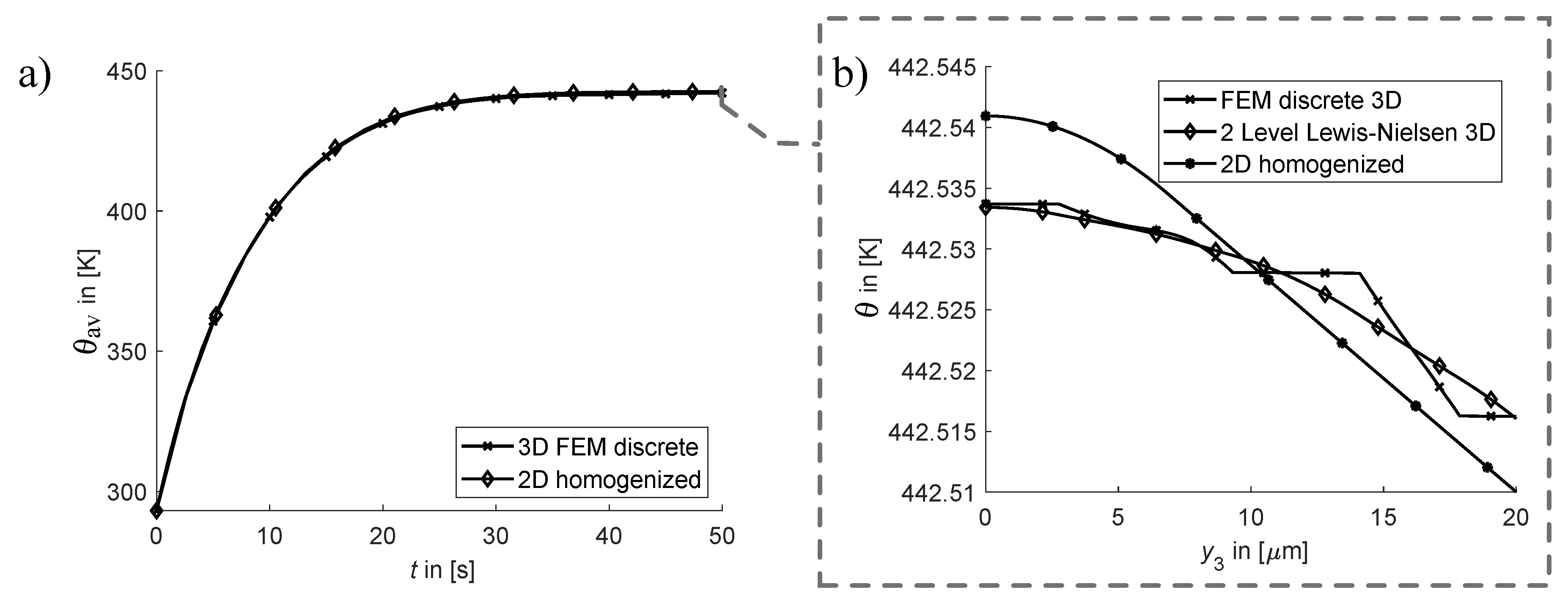
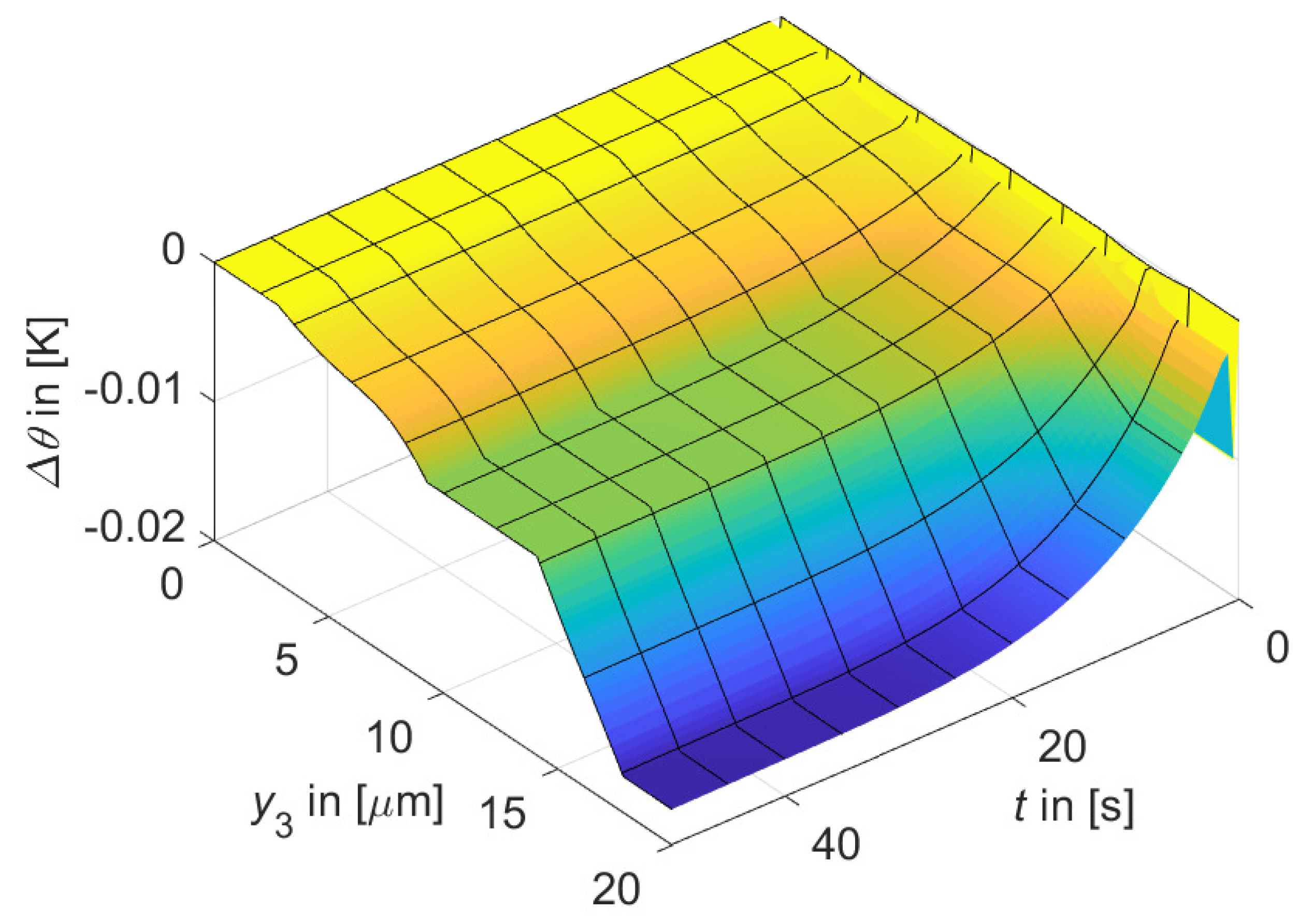
3.2. Transient Heat Flux Solution and Effects of Homogenization

The instationary heat flux problem is especially relevant for heat up and cool down processes, which appear typically in tailored thermal management applications, e.g., the intervall controlled de-icing of wing leading edges of aircraft. Also the efficient but accurate calculation of the instationary problem is important to fit the thermal management function to requirements in future multifunctional structures.
Figure 5 shows the temperature difference (compare Equation (44)) over time and over the thickness coordinate y 3 , calculated from the discrete RVE representation of the PeCCF composite material. It should be noted, that the temperature difference was reduced by the maximum temperature at each time step. The temperature gradient in thickness direction increases over time, since the overall temperature increases. Accordingly, the influence of this temperature difference is most significant for the stationary case. The step in the plotted surface at t = 0.5 s is related to the numerical solution process, where the effect of sudden joule heating excites the temperature. This effect vanishes for the following time steps. Accordingly, the interpretations from Section 3.1 are supported by the transient solution based on the discrete representation. Further analysis is conducted towards the homogenized approach.
Table 5 shows the effective specific heat and density, calculated by the volume average in the FEM model and the parallel ROM method comprising similar approaches. Since these material properties are volume related and direction independent, both measures are expected to provide the best effective quantity. Since ROM parallel and series method represent the whole parameter range, upper and lower bound respectively, the effect of both homogenization methods can be discussed based on the resulting transient temperature evolution.
The transient calculation is based on bc case 2, as already defined in Section 2.3 and Section 3.1 and the effective specific heat conductivity calculated from the Two-Level Lewis-Nielsen method λ = 0.43 [ W m · K ] is applied (compare Section 3.1).
In Figure 6, the resulting heat up process with Figure 6a the variation of the effective specific heat c and Figure 6c the variation of the effective density ρ are displayed in comparison to the discrete FEM solution. In both plots, the volume averaged temperature T av over the RVE is given vs. time t. For a refined insight, the temperature distribution in y 3 direction is indicated for the time step t = 10 s in Figure 6b,d respectively. The curves show, that the effective quantities from the volume average result in a slightly increased temperature. The effective properties calculated from the ROM series method result in a more increased temperature level. For both material properties, the influence on the heat up process is small compared to the resulting stationary temperature at t 50 s . In addition, the influence of specific heat and density vanishes for the stationary case (compare Equations (6) and (8)). Accordingly, the calculation of transient heat flux problems of the PeCCF composite material with the effective specific heat and density from the ROM parallel method results in conservative but accurate temperature evolutions. The heat up rate shows only minor differences to the discrete case. For calculations of the heat up process on the macro-scale, e.g., homogenized composite structures, the application of the volume averaged effective specific heat and density will predict the temperature evolution accuratley but also efficient in terms of computational cost. Especially the increase of computational efficiency will be discussed in the following chapter, where the model reduction from 3D to 2D is reported and benefits are highlighted.

3.3. Accuracy of 2D Reduced Model

The reduction of the RVE 3D model for the stationary and instationary heat flux problem is motivated by the fact, that the laminates’ thickness is more than two orders in magnitude smaller than its edge length. Accordingly, the main direction of heat flux is the thickness direction. The effective directions of joule heating and the heat flux problem are the y 1 direction for electrical current conduction and the y 3 direction for the heat conduction. The following results are related to the assumptions given in Section 2.5.
Figure 7 presents (a) the transient temperature evolution and (b) the stationary temperature distribution in thickness direction y 3 of the 2D model in direct comparison to the discrete 3D model. The 2D transient results (Figure 7a) shows, as expected from results discussion in Section 3.2, no singificant difference compared to the 3D transient results. The representation of the material in y 2 direction by equivalent thicknesses d a and d e q , as assumed in Section 2.5, shows a good representation of the transient themal behaviour. Apart from the instationary case, the stationary temperature distribution in (Figure 7b) shows significant differences from the 3D discrete and 3D homogenized case. Here the geometric reduction from 3D to 2D increases the temperature gradient across the thickness direction. Although the temperature level is similar, the averaged temperature drop over thickness is 1.5 K mm , which is an increase compared to the discrete model of 50%. With respect to future applications of the reduced 2D thermal model in coupled thermo-mechanical models for PeCCF composites, the description of the temperature distribution in thickness direction can be classified as conservative.
The motivation for the model reduction was the increase of model efficiency in terms of computational cost. Table 6 indicates the calculation times on the reference system for transient and stationary analysis for the different level of complexity. The homogenization of the microstructure within the 3D model and the dimension reduction lead to a huge reduction of computational cost of up to 97 %. From this perspective, the application of the homogenized, reduced model in multiscale simulation models is extremely beneficial. However, the epectation of a conservative resulting temperature distribution in the reduced 2D model needs to be taken into account for coupled multiphysics models.

4. Conclusions

The objective to characterize and compute the thermal behaviour of polymer electrolyte coated carbon fibre composites efficiently was indicated to be important with respect to multifunctional applications. Especially the coupled electro-thermo-mechanical modelling in a multiscale approach requires a well defined homogenized representation of the thermal problem. The analysis of effective composite material properties and model reduction strategies in terms of heat flux behaviour is presented in this paper for the first time. In direct comparison to the discrete RVE model solution the following conclusions are made, which highlight the novelty of this work:
  • Based on the discrete RVE representation of the PeCCF composite on the microscale a characteristic temperature gradient in the transversal plane of Δ θ = 1.0 K mm was indicated for heat convection at the surface. It should be noted, that this number is a linear average. The discrete temperature gradient could be larger. This property is important, as such a thermal gradient in the thickness direction of a typical laminate could lead to additional thermal stresses within the laminate plies. Such temperature gradients have been neglected in earlier studies on PeCCF composite materials. With this new recognition it is expected that the temperature distribution within the material plays an important role for the mechanical performance.
  • The influence of the solid polymer electrolyte coating on the transversal heat flux was identified to be small, since the thermal properties are in the range of the matrix material and the volume fraction of this domain is small. Especially in the transversal plane the effective length of the coating (the thickness) is small, which reduces the temperature drop in its domain. However, since the coating represents an additional interphase, the fibre volume fraction is geometrically limited by the presence of the coating layer. This leads to smaller fibre volume fractions, which induces a smaller thermal conductivity in the transversal plane compared to classical carbon fibre—matrix composites. Accordingly, a high fibre volume ratio in PeCCF composites is needed for improved thermal conductivity.
  • The homogenization of the thermal conductivity λ in the transversal plane was found to be best by the Three-Phase Lewis-Nielsen method and the new Two-Level Lewis-Nielsen approach. The resulting stationary temperature distributions in the transversal plane are compared to those resulting from virtually measured thermal conductivities. Both methods represent narrow lower and upper bounds respectively. The new Two-Level Lewis-Nielsen approach enabled tailoring the effect of the coating by including its geometric appearance on particle level (PeCCF level). Based on the effective thermal conductivity, a suitable and efficient prediction of temperature distributions and temperature gradients are enabled. This new method directly addresses the special geometric composition of the PeCCF compound and is therefore very accurate to predicit the thermal conductivity in the transversal plane.
  • The homogenization of specific heat c and density ρ were identified best by the volume average, based on the RVE model, and the parallel ROM method, which are similar approaches. Both quantities showed minor influence on the transient heat up process. The discrete temperature difference at a certain time step during heat up was small compared to the resulting stationary temperature. Accordingly, the application of effective properties in a homogenized material representation has negligible influence on the prediction of the transient heat flux problem.
  • With respect to the macroscale (laminate of PeCCF composite), the thickness direction governs the heat flux, since heat convection only appears at the surfaces of the laminate. While joule heating is effective only in longitudinal direction, the width direction is uneffected from both physical effects. In a newly proposed reduced 2D approach for the microscale, a simplified and accurate prediction of the thermal field in transversal direction was demonstrated. The homogenized and reduced 2D model in the y 1 , y 3 plane showed a more conservative representation of the temperature gradient of Δ θ = 1.5 K mm . Compared to the discrete 3D model, this difference is reduced to the fact, that in the 3D representation a discrete heat source distribution is given by the fibre distribution. This is vanished in the reduced model and replaced by a continous heat source distribution. This allows no heat exchange in width direction which effects the resulting temperature field. However, in terms of computational cost, the 2D model was up to 97% more efficient compared to the discrete model, which is a huge benefit of this new approach. This is especially important for future coupled multiscale models. Accordingly, the more conservative temperature distribution can be accepted in order to provide an efficient modelling approach for the microscale thermal heat flux problem.
  • With respect to applications, the representation of the PeCCF composite material with homogenized material constants in the thermal problem will be of importance. Applications such as structural batteries, thermal management structures and composites with adaptive stiffness will be subjected to significant joule heating during electrical current conduction. The efficient predicition of the thermal field is crucial for the multiphysically coupled modelling of such multifunctional materials. The described approaches and results pave the way for the coupled representation of the thermo-mechanical behaviour of the PeCCF composite.
Results and conclusions presented in this work are based on the assumption of ideal contact between the single domains resulting in zero interfacial thermal resistance. This assumption was well motivated from foregoing conclusions in literature. However, this assumption could lead to overestimates of the thermal performance of the composite material. However, the presented approach for the thermal problem enables the analysis of the coupled thermo-mechanical behaviour of the PeCCF composite. This is of special interest, since the authors already indicated a significant stiffness drop of the composite based on the thermal dependent stiffness of the SPE coating.

5. Future Research

The assessment of the quality of domain interfaces and its influence on the thermal conductivity needs to be subject of future research. Numerical studies by Kaminski and Ostrowski [20] highlighted the influence of interfacial defects on effective thermal conductivity, which supports the need for experimental interface characterization. Furthermore, the thermal conductivity and the specific heat of the PeCCF composite are important to be determined experimentally. A direct comparison with the numerical results of this study can validate the homogenization method. The numerical thermal model of the PeCCF composite will be developed further towards a thermo-mechanically coupled material model, which will be part of the future work of the authors. Thereby, effects from temperature rise and temperature gradients on the mechanical performance of the material will be studied.

Author Contributions

Conceptualization, all; methodology, M.O.H.S.; software, M.O.H.S.; validation, M.O.H.S.; investigation, M.O.H.S.; resources, all; data curation, M.O.H.S.; writing—original draft preparation, M.O.H.S.; writing—review and editing, T.K. and H.P.M.; visualization, all; supervision, T.K. and H.P.M. All authors have read and agreed to the published version of the manuscript.

Funding

This research received no external funding.

Institutional Review Board Statement

Not applicable.

Informed Consent Statement

Not applicable.

Data Availability Statement

All needed data for reproduction of results is contained within the article. The data presented in this study can be reproduced by given assumptions and equations.

Acknowledgments

M.O.H. Schutzeichel acknowledges valuable discussions about thermal behaviour of multifunctional composites with David Carlstedt from Chalmers University of Technology, Gothenburg, Sweden.

Conflicts of Interest

The authors declare no conflict of interest.

Abbreviations

The following abbreviations are used in this manuscript:
PeCCFPolymer electrolyte coated carbon fibre
SPEStructural polymer electrolyte
RVERepresentative volume element
BCBoundry condition
FEMFinite element method
DMFdimethylformamide
ROMRule of mixtures

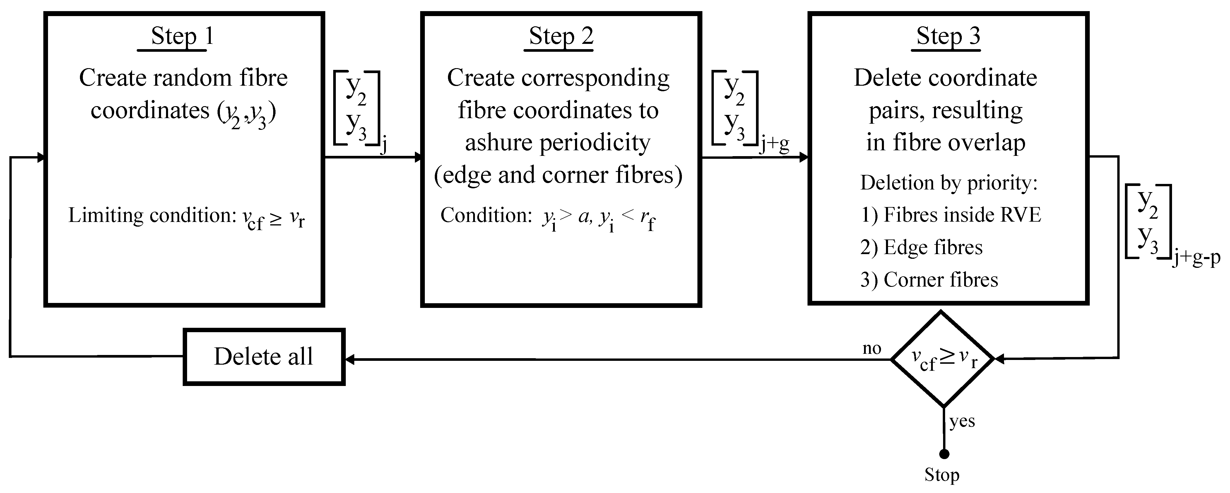
Appendix A. RVE Generation Algorithm

The algorithm for a random fibre distribution is implemented in Matlab, which generates center coordinates in the transversal plane. Figure A1 presents the 3 major steps for the generation of fibre coordinates.
Figure A1. Algorithm for RVE generation with random fibre distibution.
Applmech 02 00043 g0a1
Step 1 results in a number j of coordinate pairs in the transversal plane, which are distributed randomly. The number j is limited by the desired fibre volume ratio v r . In step 2 the resulting coordinate pairs are checked for the condition that the resulting fibre is overlapping with an edge or a corner. This is checked by the distance between fibre coordinates and the boundaries’ position. All edge fibre coordinates are repeated on the opposite boundary, such that the cut part of the fibre is included on the opposite face inside the RVE. In case of corner-overlapping fibres, new coordinates are created to represent the cut parts on all other corners. This results in an additional number of coordinate pairs g. Step 3 checks, which fibres are overlapping with others by comparing always two fibres. One of the two fibres is deleted with the given priority, in order to ashure the geometric periodicity after deletion. Accordingly, the number of coordinate pairs is reduced by a number p of deletions.
Finally the remaining fibre volume ratio is checked, in order to prove that the requirement of step 1 is still fulfilled. If this requirement is not achived, the whole process is repeated, else the algorithm stops. The resulting coordinates are then transferred with Matlab LiveLink to Comsol for RVE geometry creation. This algorithm performs fast and fulfills the required accuracy to include periodic boundary conditions in COMSOL for opposite domain faces. Figure A2 shows the applied example of this study with the resulting coordinate pair distribution from the algorithm (a) and the corresponding 3D RVE generated in COMSOL (b).
Figure A2. Geometry generation example: (a) The resulting coordinate pair distribution and (b) Corresponding 3D RVE.
Applmech 02 00043 g0a2

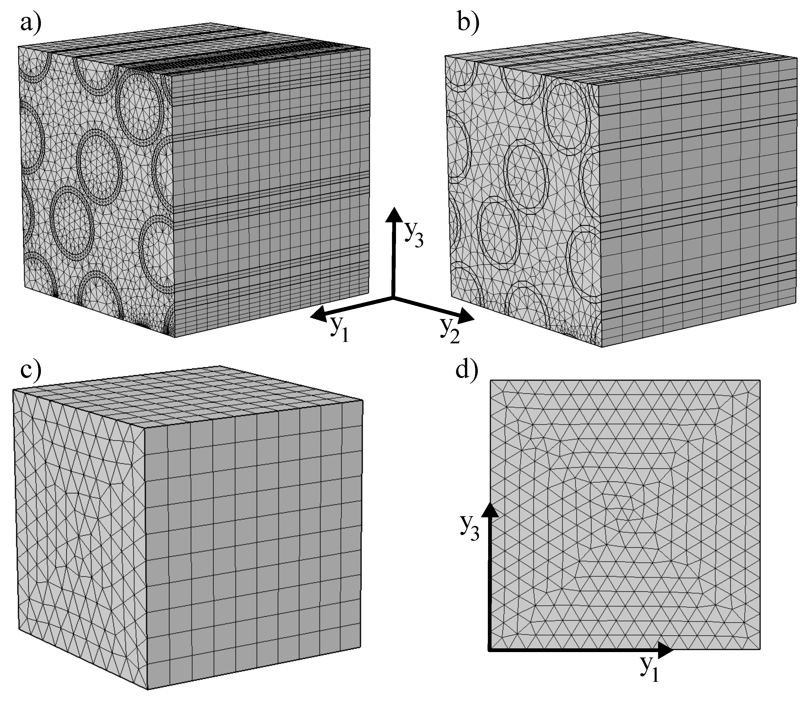
Appendix B. Technical Data on FEM Discretization

This section presents the technical details on the FE meshes applied in all studies. Figure A3a,b present two possible meshes M1 and M2 (see data in Table A1) which are analysed towards accuracy of results. All meshes are built by a triangular mesh on the surface ( y 2 y 3 , transversal plane) and extruded in y 3 direction, which results in prismatic elements with triangular base area. The shape functions are defined to be quadratic, in order to represent the circular geometry faces in the discrete representations of the RVEs. All calculations within this study are done with both mesh geometries. Results are compared and no influence by the mesh is indicated. Accordingly, mesh M2 is applied further for analysis referred to as “FEM discrete”, as it reduces computational cost significantly.
Figure A3. Mesh geometries for FEM calculations: (a) Refined mesh M1, (b) Coarse mesh M2, (c) Homogenized RVE mesh M3 and (d) 2D mesh M4; The coordinate origin is placed at the hidden corner.
Applmech 02 00043 g0a3
Table A1. Technical details of FE meshes M1-M4 compare Figure A3.
PropertiesMesh M1Mesh M2Mesh M3Mesh M4
Element typesPrismaTriangle
Shape functionsQuadratic serendipity *
Reference fibre volume ratio v c f 0.55--
Nr. of elements domain 115,3713090--
Nr. of elements domain 228,1962670--
Nr. of elements domain 319,0574490--
Total nr. of elements62,62410,2502560578
Total degrees of freedom (DOF)168,20629,21675731217
* as defined in COMSOL MULTIPHYSICS v5.5.
The remaining mesh geometries are applied for model reduction purposes, e.g., in case of homogenized material constants and a reduction to a 2D approach in the y 1 y 3 plane (see Figure A3 M3 and M4 respectively). It should be noted, that the reduced meshes are only applied to homogenized material properties and results are discussed with respect to discrete solutions, based on meshes M1 and M2. Accordingly, in this study, all results are referred to the given fibre volume ratio of v c f = 0.5 . However, meshes M3 and M4 can also be used for calculations based on homogenized material properties from other fibre volume ratios. It is clearly indicated in Table A1, that the resulting amount of necessary elements and resulting total number of degrees of freedom is drastically reduced by homogenization in mesh M3 and dimension reduction in mesh M4. The effect on results accuracy and computational cost is discussed in main Section 3.
The technical implementation of the FEM analysis is done in Comsol Multiphysics (v.5.5). The general equations of heat transfer (see Equation (6)) and joule heat (see Equation (18)) are part of the standard physics in the basic module. To implement the boundary conditions for heat transfer given in Equations (12)–(17), adiabatic, heat flux or periodicity conditions are applied for the heat flux problem in Comsol. Furthermore, the boundary conditions for joule heat (Equations (19) and (20)) are defined by normal current density and ground condition in Comsol. Both, heat transfer and electric current physics are coupled via the multiphysics node for electromagnetic heating.

References

  1. Asp, L.E.; Greenhalgh, E.S. Structural power composites. Compos. Sci. Technol. 2014, 101, 41–61. [Google Scholar] [CrossRef]
  2. Asp, L.E.; Johansson, M.; Lindbergh, G.; Xu, J.; Zenkert, D. Structural battery composites: A review. Funct. Compos. Struct. 2019, 1, 042001. [Google Scholar] [CrossRef]
  3. Asp, L.E.; Bouton, K.; Carlstedt, D.; Duan, S.; Harnden, R.; Johannisson, W.; Johansen, M.; Johansson, M.K.G.; Lindbergh, G.; Liu, F.; et al. A Structural Battery and its Multifunctional Performance. Adv. Energy Sustain. Res. 2021, 2, 2000093. [Google Scholar] [CrossRef]
  4. Schutzeichel, M.; Linde, P. Heatable Leading Edge Apparatus, Leading Edge Heating Sysem and Aircraft Comprising Them. U.S. Patent Application No. US201916430633 20190604, 19 June 2018. [Google Scholar]
  5. Bismarck, A.; Lee, A.F.; Sarac, A.S.; Schulz, E.; Wilson, K. Electrocoating of carbon fibres: A route for interface control in carbon fibre reinforced poly methylmethacrylate? Compos. Sci. Technol. 2005, 65, 1564–1573. [Google Scholar] [CrossRef]
  6. Willgert, M.; Kjell, M.H.; Jacques, E.; Behm, M.; Lindbergh, G.; Johansson, M. Photoinduced free radical polymerization of thermoset lithium battery electrolytes. Eur. Polym. J. 2011, 47, 2372–2378. [Google Scholar] [CrossRef]
  7. Leijonmarck, S.; Carlson, T.; Lindbergh, G.; Asp, L.E.; Maples, H.; Bismarck, A. Solid polymer electrolyte-coated carbon fibres for structural and novel micro batteries. Compos. Sci. Technol. 2013, 89, 149–157. [Google Scholar] [CrossRef]
  8. Schutzeichel, M.O.H.; Kletschkowski, T.; Monner, H.P. Effective stiffness and thermal expansion of three-phase multifunctional polymer electrolyte coated carbon fibre composite materials. Funct. Compos. Struct. 2021, 3, 015009. [Google Scholar] [CrossRef]
  9. Schutzeichel, M.; Kletschkowski, T.; Linde, P.; Asp, L.E. Experimental characterization of multifunctional polymer electrolyte coated carbon fibres. Funct. Compos. Struct. 2019, 1, 025001. [Google Scholar] [CrossRef]
  10. Carlstedt, D.; Asp, L. Thermal and diffusion induced stresses in a structural battery under galvanostatic cycling. Compos. Sci. Technol. 2019, 179, 69–78. [Google Scholar] [CrossRef]
  11. Carlstedt, D.; Runesson, K.; Larsson, F.; Xu, J.; Asp, L.E. Electro-chemo-mechanically coupled computational modelling of structural batteries. Multifunct. Mater. 2020, 3, 045002. [Google Scholar] [CrossRef]
  12. Hannoschöck, N. Wärmeleitung und Transport; Springer: Berlin/Heidelberg, Germany, 2018. [Google Scholar] [CrossRef]
  13. Zhang, H.; Zhang, X.; Fang, Z.; Huang, Y.; Xu, H.; Liu, Y.; Wu, D.; Zhuang, J.; Sun, J. Recent Advances in Preparation, Mechanisms, and Applications of Thermally Conductive Polymer Composites: A Review. J. Compos. Sci. 2020, 4, 180. [Google Scholar] [CrossRef]
  14. Venetis, J.; Sideridis, E. The Thermal Conductivity of Periodic Particulate Composites as Obtained from a Crystallographic Mode of Filler Packing. J. Compos. Sci. 2018, 2, 71. [Google Scholar] [CrossRef] [Green Version]
  15. Swartz, E.T.; Pohl, R.O. Thermal boundary resistance. Rev. Mod. Phys. 1989, 61, 605–668. [Google Scholar] [CrossRef]
  16. Benveniste, Y. Effective thermal conductivity of composites with a thermal contact resistance between the constituents: Nondilute case. J. Appl. Phys. 1987, 61, 2840–2843. [Google Scholar] [CrossRef]
  17. He, B.; Mortazavi, B.; Zhuang, X.; Rabczuk, T. Modeling Kapitza resistance of two-phase composite material. Compos. Struct. 2016, 152, 939–946. [Google Scholar] [CrossRef]
  18. Tsekmes, I.A.; Kochetov, R.; Morshuis, P.H.F.; Smit, J.J. Thermal conductivity of polymeric composites—A review. In Proceedings of the 2013 IEEE International Conference on Solid Dielectrics (ICSD 2013), Bologna, Italy, 30 June–4 July 2013; pp. 678–681. [Google Scholar] [CrossRef]
  19. Nan, C.W.; Birringer, R.; Clarke, D.R.; Gleiter, H. Effective thermal conductivity of particulate composites with interfacial thermal resistance. J. Appl. Phys. 1997, 81, 6692–6699. [Google Scholar] [CrossRef]
  20. Kamiński, M.; Ostrowski, P. Homogenization of heat transfer in fibrous composite with stochastic interface defects. Compos. Struct. 2021, 261, 113555. [Google Scholar] [CrossRef]
  21. FAA. Fiber Composite Analysis and Design: Composite Materials and Laminates; National Technical Information Service: Springfield, VA, USA, 1997; Volume 1. [Google Scholar]
  22. Kochetov, R.; Andritsch, T.; Lafont, U.; Morshuis, P.H.F.; Picken, S.J.; Smit, J.J. Thermal behaviour of epoxy resin filled with high thermal conductivity nanopowders. In Proceedings of the 2009 IEEE Electrical Insulation Conference, Montreal, QC, Canada, 31 May–3 June 2009; IEEE Service: Piscataway, NJ, USA, 2009; pp. 524–528. [Google Scholar] [CrossRef]
  23. Kaminski, M.; Pawlik, M. Homogenization of Transient Heat Transfer Problems for Some Composite Materials. In Proceedings of the Sixth International Conference on Computational Structures Technology; Topping, B., Bittnar, Z., Eds.; Civil-Comp Press: Stirlingshire, UK, 2002. [Google Scholar] [CrossRef]
  24. Kim, H.; Ji, W. Thermal conductivity of a thick 3D textile composite using an RVE model with specialized thermal periodic boundary conditions. Funct. Compos. Struct. 2021, 3, 015002. [Google Scholar] [CrossRef]
  25. Loos, M. Fundamentals of Polymer Matrix Composites Containing CNTs. In Carbon Nanotube Reinforced Composites; Elsevier: Amsterdam, The Netherlands, 2015; pp. 125–170. [Google Scholar] [CrossRef]
  26. Kochetov, R.; Korobko, A.V.; Andritsch, T.; Morshuis, P.H.F.; Picken, S.J.; Smit, J.J. Three-phase lewis-nielsen model for the thermal conductivity of polymer nanocomposites. In 2011 Annual Report Conference on Electrical Insulation and Dielectric Phenomena; IEEE: Cancun, Mexico, 2011; pp. 338–341. [Google Scholar] [CrossRef]
  27. Bargmann, S.; Klusemann, B.; Markmann, J.; Schnabel, J.E.; Schneider, K.; Soyarslan, C.; Wilmers, J. Generation of 3D representative volume elements for heterogeneous materials: A review. Prog. Mater. Sci. 2018, 96, 322–384. [Google Scholar] [CrossRef]
  28. Leijonmarck, S. Preparation and characterization of Electrochemical Devices for Energy Storage and Debonding. Ph.D. Thesis, KTH School of Engineering Sciences, Stockholm, Sweden, 2013. [Google Scholar]
  29. Tenax, T. Delivery Programme and Characteristics for Tenax Filaments; Technical Report; Toho Tenax Europe GmbH: Wuppertal, Germany, 2017. [Google Scholar]
  30. Bertram, A.; Glüge, R. Solid Mechanics—Theory, Modeling and Problems; Springer International Publishing: Berlin/Heidelberg, Germany, 2015. [Google Scholar]
  31. Pradere, C.; Batsale, J.C.; Goyhénèche, J.M.; Pailler, R.; Dilhaire, S. Thermal properties of carbon fibers at very high temperature. Carbon 2009, 47, 737–743. [Google Scholar] [CrossRef]
  32. Mark, J.E. Physical Properties of Polymers Handbook, 2nd ed.; Springer: New York, NY, USA, 2007. [Google Scholar] [CrossRef] [Green Version]
  33. Carlson, T. Multifunctional Composite Materials—Design, Manufacture and Experimental Characterization. Ph.D. Thesis, Lulea University of Technology, Lulea, Sweden, 2013. [Google Scholar]
  34. Carlstedt, D.; Marklund, E.; Asp, L. Effects of state of charge on elastic properties of 3D structural battery composites. Compos. Sci. Technol. 2019, 169, 26–33. [Google Scholar] [CrossRef] [Green Version]
  35. Ihrner, N.; Johannisson, W.; Sieland, F.; Zenkert, D.; Johansson, M. Structural lithium ion battery electrolytes via reaction induced phase-separation. J. Mater. Chem. A 2017, 5, 25652. [Google Scholar] [CrossRef] [Green Version]
  36. Willgert, M.; Kjell, M.H.; Johansson, M. Effect of Lithium Salt Content on the Performance of Thermoset Lithium Battery Electrolytes. In Polymers for Energy Storage and Delivery: Polyelectrolytes for Batteries and Fuel Cells; American Chemical Society: Washington, DC, USA, 2012; pp. 55–65. [Google Scholar] [CrossRef]
  37. Hughes, J. The carbon fibre/epoxy interface—A review. Compos. Sci. Technol. 1991, 41, 13–45. [Google Scholar] [CrossRef]
  38. Vasiliev, V.V.; Morozov, E.V. Advanced Mechanics of Composite Materials and Structural Elements, 3rd ed.; Elsevier: Amsterdam, The Netherlands, 2013. [Google Scholar] [CrossRef]
  39. Nielsen, L.E. Generalized Equation for the Elastic Moduli of Composite Materials. J. Appl. Phys. 1970, 41, 4626–4627. [Google Scholar] [CrossRef]
  40. Lewis, T.B.; Nielsen, L.E. Dynamic mechanical properties of particulate-filled composites. J. Appl. Polym. Sci. 1970, 14, 1449–1471. [Google Scholar] [CrossRef]
Figure 1. Assumptions for composite material domains, domain interfaces and discussed directions referred to the macroscale (laminate).
Applmech 02 00043 g001
Figure 2. RVE with fibre volume ratio v c f = 0.5 , boundary face indicators ( Y i ), and global coordinate system y i with i = 1, 2, 3.
Applmech 02 00043 g002
Figure 3. Schematic of the Two-level Lewis-Nielsen approach, applying the method first on particle level (level 1) and second on particle filled matrix level (level 2), Equation indices are given with respect to the material phase or mixture.
Applmech 02 00043 g003
Figure 4. Temperature distribution corresponding to BC case 2; (a) Isotherms in RVE, (b) Temperature distributions along y 3 axis ( ( y 1 , y 2 ) = ( 10 μ m , 10 μ m ) ), (c) Temperature difference related to respective maximum Temperature ( ( y 1 , y 2 ) = ( 10 μ m , 10 μ m ) ).
Applmech 02 00043 g004
Figure 5. Transient evolution of temperature difference in thickness direction y 3 over time based on the discrete RVE model.
Applmech 02 00043 g005
Figure 6. Transient heat up process of the RVE with volume averaged temperature T av ; (a) Variation of effective specific heat c , (b) Temperature distribution along y 3 axis ( ( y 1 , y 2 ) = ( 10 μ m , 10 μ m ) , t = 10 s ), (c) Variation of effective density ρ , (d) Temperature distribution along y 3 axis ( ( y 1 , y 2 ) = ( 10 μ m , 10 μ m ) , t = 10 s ).
Applmech 02 00043 g006
Figure 7. Comparison between 3D discrete and 2D homogenized and reduced model; (a) Transient heat up process, (b) Stationary Temperature distribution along y 3 axis ( y 1 = 10 μ m ).
Applmech 02 00043 g007
Table 1. Geometric parameters.
PropertySymbolValueReference
RVE edge lengtha20 μmchosen
Diameter carbon fibres * d f 5.0 μm[28,29]
SPE coating thickness t c 0.5 μm[28]
* referred to IMS65 carbon fibres.
Table 2. Material properties of domains Ω 1 Ω 3 (see Figure 2).
DomainSym.ValueUnitExplanationReference
Ω 1 : Carbon
Fibre IMS65
ρ 1 1.78 g cm 3 Density[29]
λ 1 50 W m · K Thermal conductivityassumed based on [21]
c 1 1400 J kg · K Specific heat capacityassumed based on [31]
κ 1 1.45 · 10 3 Ω · cm Specific electrical resistance[9]
Ω 2 : Coating * ρ 2 1.3 g cm 3 Density[10]
λ 2 0.21 W m · K Thermal conductivity[32]
c 2 2090 J kg · K Specific heat capacity[32]
κ 2 Ω · cm Specific electrical resistance** assumed
Ω 3 : Matrix ρ 3 1.3 g cm 3 Density[21]
λ 3 0.19 W m · K Thermal conductivity[32]
c 3 1050 J kg · K Specific heat capacity[32]
κ 3 Ω · cm Specific electrical resistance** assumed
* SPE coating made from 1:1 SR550:SR209 with 8% li-triflate dissolved in DMF; ** Assumed based on the fact that the electrical conducitivity is much; smaller compared to carbon fibre IMS65.
Table 3. Summary of volume ratios related to present RVE geometry.
Volume RatiosSymbolValueReference Volume
Fibre volume ratio v f 0.34RVE
Coating volume ratio v c 0.16RVE
Matrix volume ratio v m 0.50RVE
Coated fibre volume ratio v c f 0.49RVE
Particle fibre volume ratio v p f 0.69PeCCF *
Particle coating volume ratio v p c 0.31PeCCF *
* Total volume of one polymer electrolyte coated carbon fibre.
Table 4. Effective thermal conductivities calculated from respective methods and input parameter.
Method k = λ in [ W m · K ] Input ParametersSubsectionComment
Volume average17.30-Section 2.4.1based on RVE
Series (ROM)0.29Table 3Section 2.4.2
Parallel (ROM)17.30Table 3Section 2.4.2
Three-Phase0.40 A = 6.6 Section 2.4.3Maximum square
Lewis-Nielsen v max = 0.79 package assumed
Two-Level
Lewis-Nielsen
0.43 A = 6.6 Section 2.4.4Maximum square
package assumed
v max = 0.79
A p f = 0.1
v p f , max = 1
Virtually measured λ = [ λ 1 , λ 2 , λ 3 ] T = [ 17.30 , 0.41 , 0.42 ] T [ W m · K ] ; BC Case 1; Section 2.2
Table 5. Effective specific heat and density calculated from respective methods.
Method k = c in [ J kg · K ] k = ρ in [ g cm 3 ] Input Para.Subs.Comment
Volume average1327.501.46-Section 2.4.1based on RVE
Series (ROM)1251.701.43Table 3Section 2.4.2
Parallel (ROM)1327.501.46Table 3Section 2.4.2
Table 6. Computation times for different levels of model complexity (reference computer system).
Computation Time in [s]
ModelTransient ProblemStationary Problem
3D discrete450137
3D homogenized176
2D homogenized145
Relative reduction of
computational cost
≈97%≈96%
Publisher’s Note: MDPI stays neutral with regard to jurisdictional claims in published maps and institutional affiliations.

