Equivalent Shell Model of Elastic Gridshells Including the Effect of the Geometric Curvature


Abstract
:1. Introduction
2. Materials and Methods
2.1. The Constitutive Identification
2.1.1. Methodological Premise
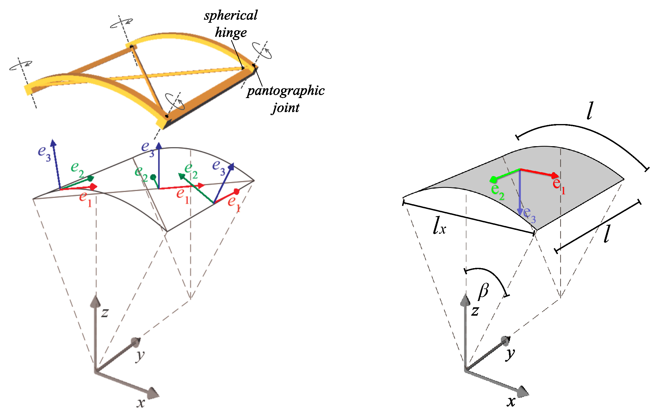
2.1.2. The Fine and the Coarse Models: The REV
2.1.3. The Localization Operator
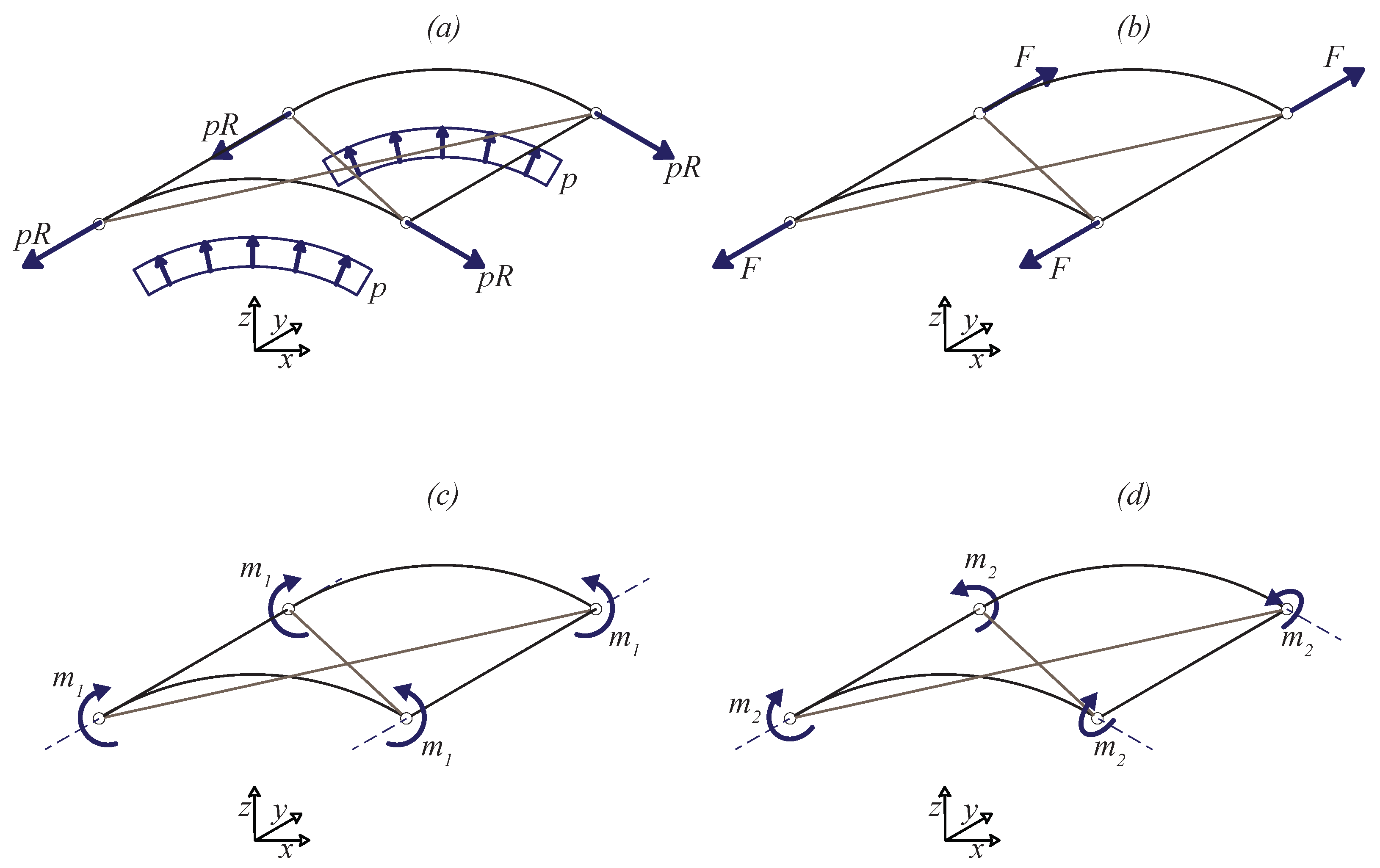
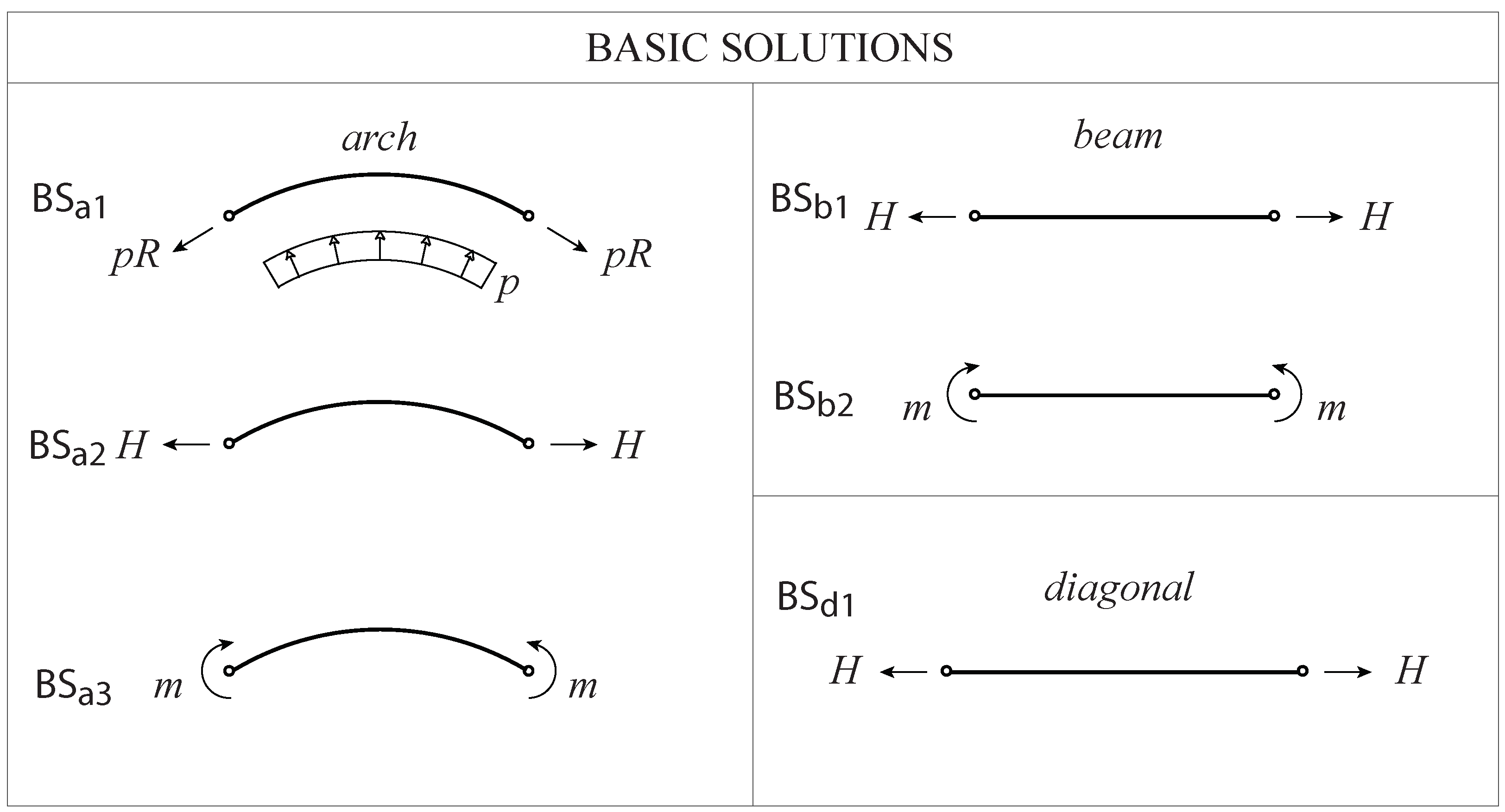
- 1.
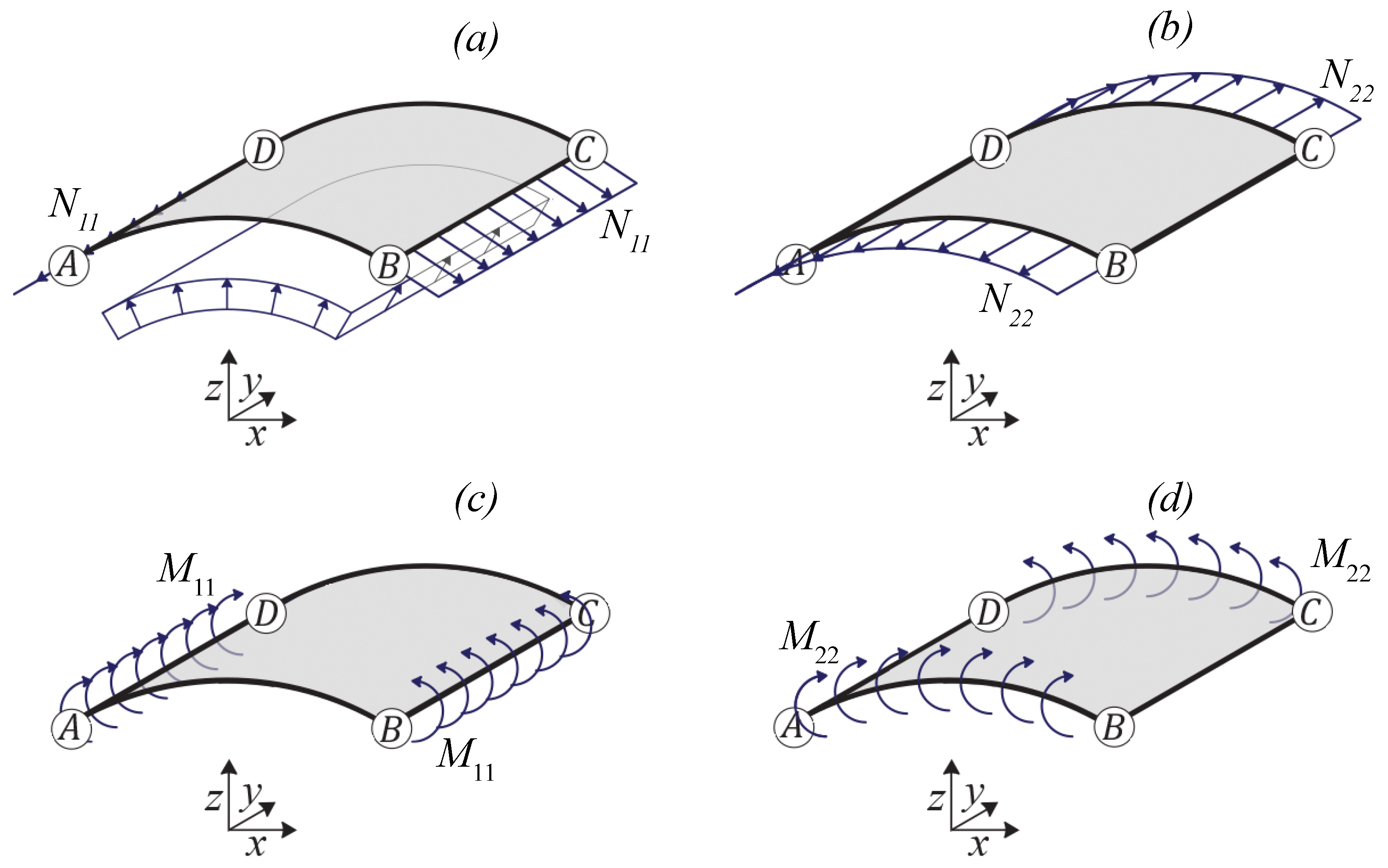
- Uniform pressure p applied to the arches in the plane , in equilibrium with the tensile forces at the end sections of the arches (Figure 3a);
- 2.
- Tensile forces F applied at the end sections of the straight beams (Figure 3b);
- 3.
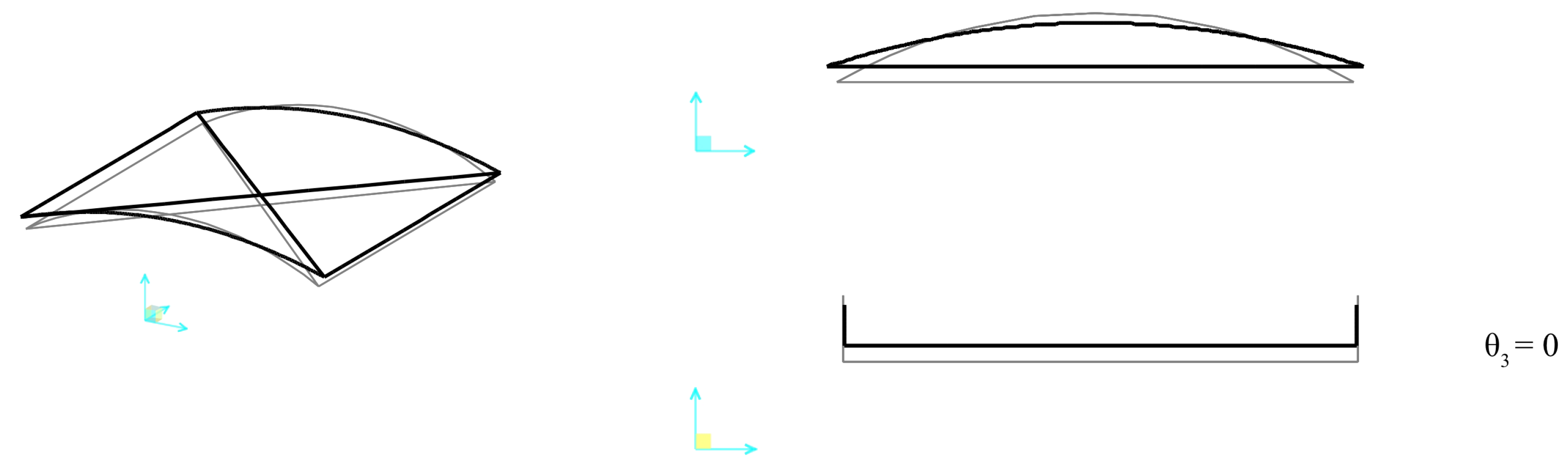
- Couples applied at the end sections of the arches (Figure 3c);
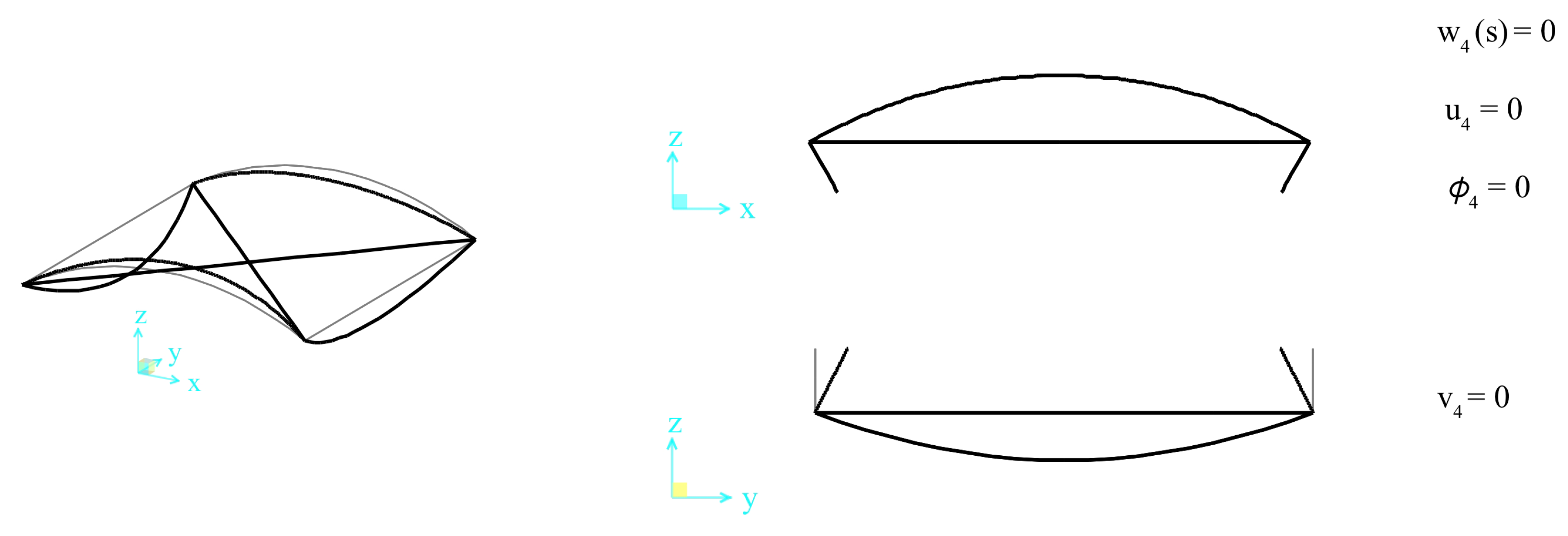
- 4.
- Couples applied at the end sections of the straight beams (Figure 3d).
2.1.4. Work Equality and the Elastic Coefficients
2.2. The Solutions of the Fine Model
- 1.
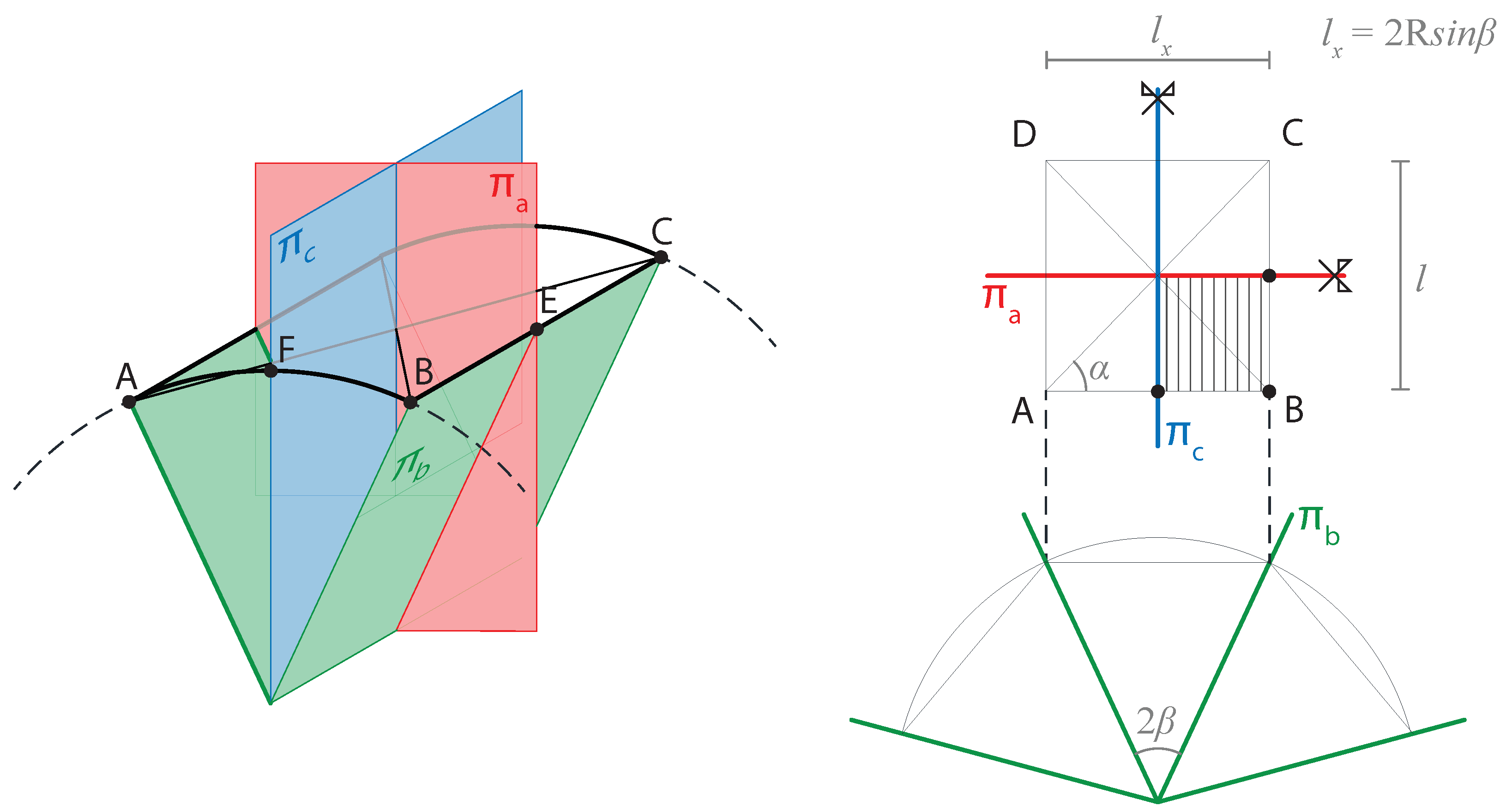
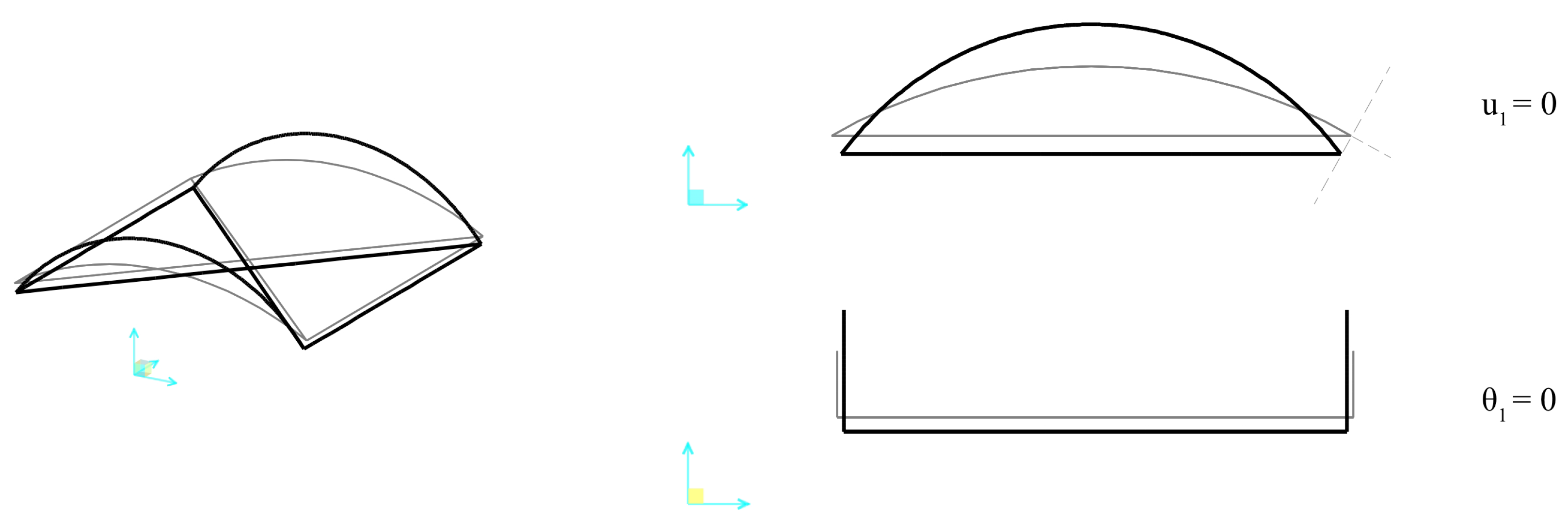
- Solving the sub-problem consisting of one half arch, one half diagonal and one half beam converging in the node B (see the rectangular hatched area in Figure 4);
- 2.
- Assuming that the displacement of the node B belong to the plane .
2.3. The Solution Method
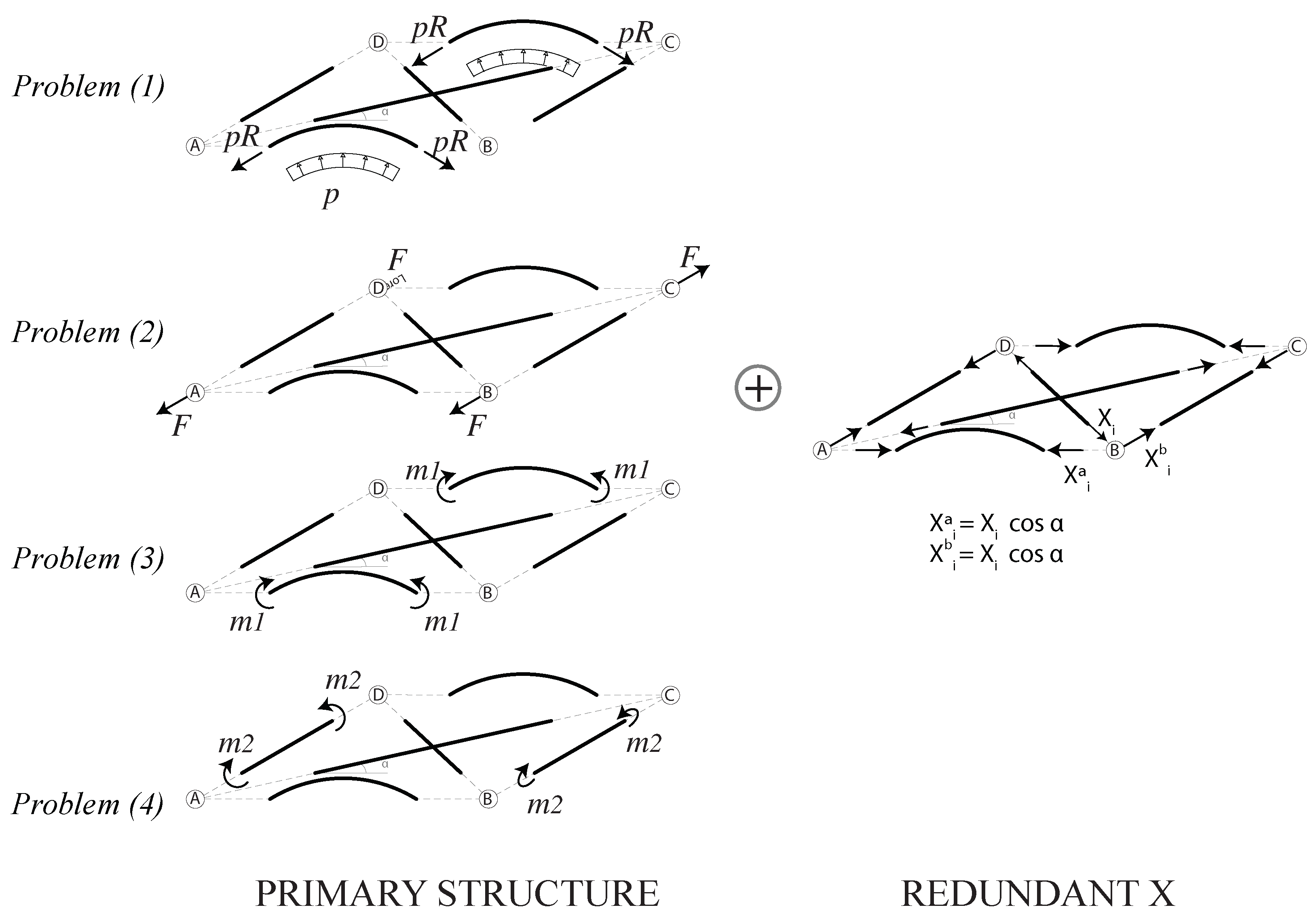
- The axial force in the diagonal is assumed as redundant reaction (see Figure 5).
- The redundant reaction is projected onto the vertical plane containing the arch and in the plane containing the beam, by obtaining the components and , respectively, where is the angle formed between the diagonal and the plane in the reference configuration.
- Five statically determined elastic traction sub-problems are solved:
- : The arch subject to the external loads (if present);
- : The arch subject to ;
- : The beam subject to the external loads (if present);
- : The beam subject to ;
- : The diagonal subject to .
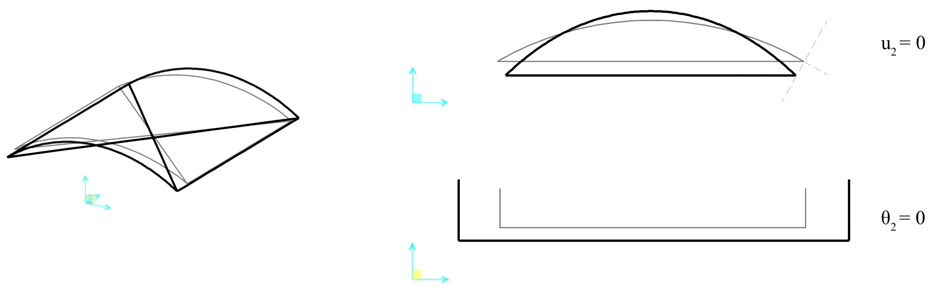
- For each sub-problem the following six constraints are assumed on the plane displacements of the half arch and half beam:
- The plane displacements of the arch are obtained as sum of the results of the problems and , the plane displacements of the beam are obtained as sum of the results of the problems and , while the displacements of the diagonal comes from the solution of the problem . All the displacements are written in terms of .
- The compatibility condition between the axial displacement of the diagonal and the projection of the axial displacements of arch and beam on the x-y plane is used in order to find the value of .
- The whole displacement field for each element is finally written in terms of the external load only.
2.3.1. The Equations of the Three Plane Problems
2.3.2. Solution of the Problem (1)
2.3.3. Solution of the Problem (2)
2.3.4. Solution of the Problem (3)
2.3.5. Solution of the Problem (4)
2.4. The Identified Constitutive Coefficients
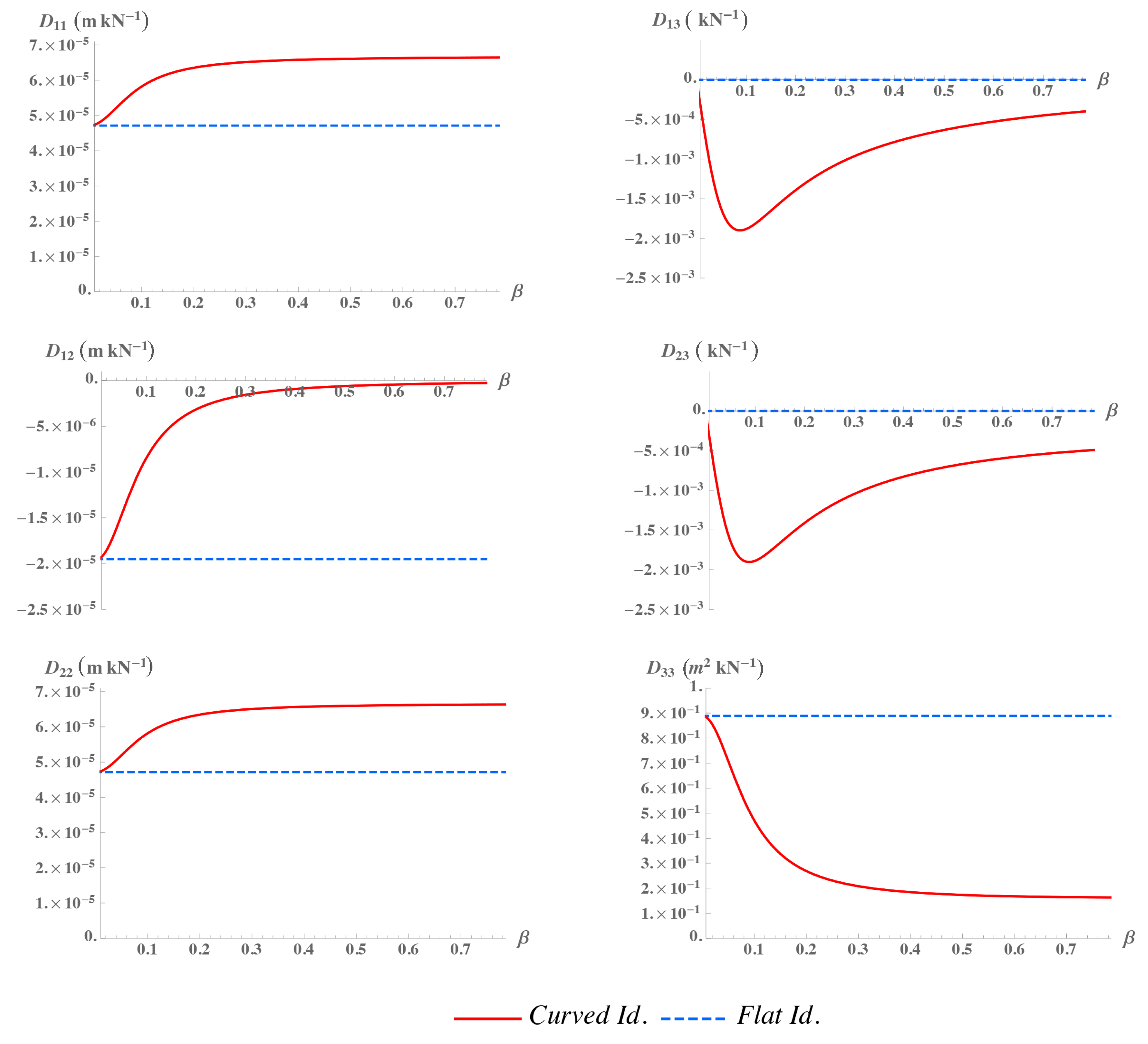
- For (flat REV) the values coincide with that of [6].
- For there is no coupling between membrane and flexural behaviour, i.e., .
- For (curved REV) the membrane coefficients and assume positive values increasing monotonically with , while the mixed membrane coefficient (Poisson effect) assume negative values whose absolute value decreases with . Then the overall membrane stiffness increases with the curvature of the REV.
- For (curved REV) the coupling coefficients , are non monotonic functions of , then there exists a value of giving the maximum coupling.
- The flexural coefficient is not affected by because we assumed a geometry curved only in x direction.
3. Results
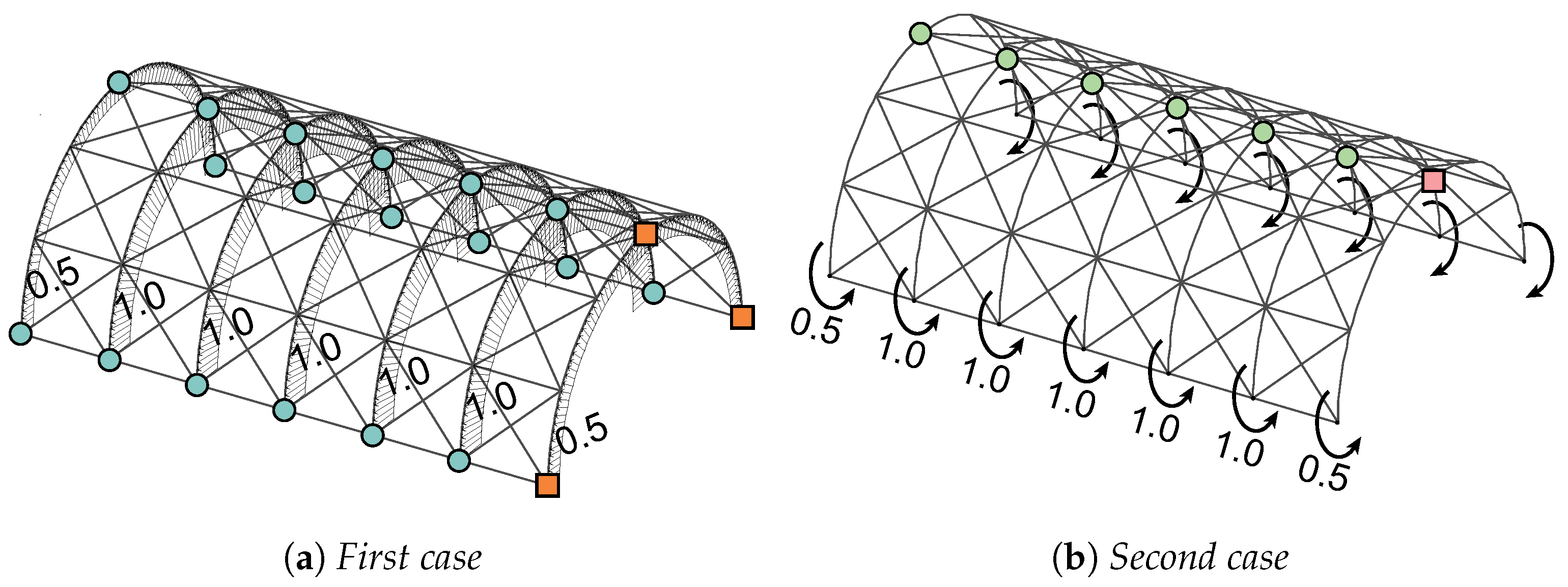
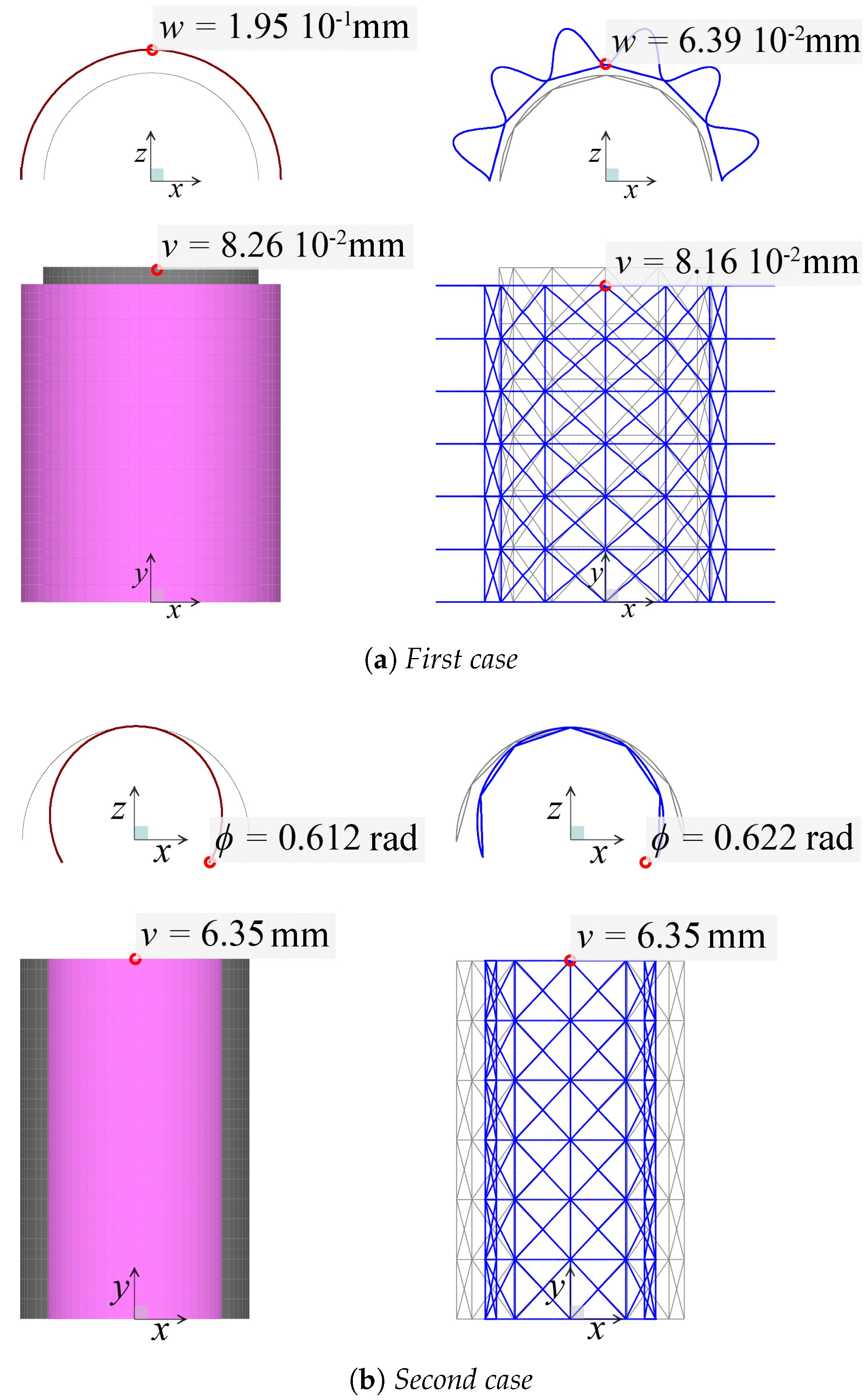
3.1. Homogeneous Load Case
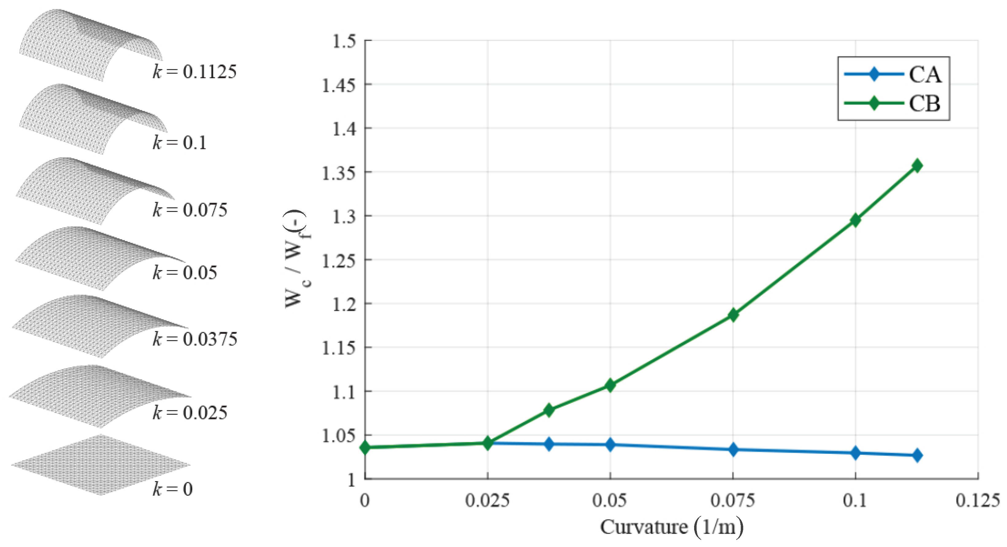
3.2. Influence of the Curvature: A Non–Homogeneous Example
4. Conclusions
Author Contributions
Funding
Institutional Review Board Statement
Informed Consent Statement
Data Availability Statement
Conflicts of Interest
References
- Preisinger, C. Linking Structure and Parametric Geometry. Archit. Des. 2013, 83, 110–113. [Google Scholar] [CrossRef]
- Zhu, B.; Fenga, R. Collapse Analysis of Single-Layer Grid Shells Based on Discrete Solid Element Method. In Proceedings of the IASS Annual Symposium, Boston, MA, USA, 16–20 July 2018. [Google Scholar]
- Goldbach, A.-K.; Bauer, A.M.; Wüchner, R.; Bletzinger, K.-U. CAD-Integrated Parametric Lightweight Design with Isogeometric B-Rep Analysis. Front. Built Environ. 2020, 6, 44. [Google Scholar] [CrossRef]
- Wright, D.T. Membrane forces and buckling in reticulated shells. J. Struct. Div. ASCE 1965, 91, 173–201. [Google Scholar] [CrossRef]
- Buchert, K.P. Buckling of Doubly Curved Orthotropic Shells. In Engineering Experiment Station; University of Missouri: Columbia, MO, USA, 1965. [Google Scholar]
- Matescu, D.; Gioncu, V.; Konrad, C. Stability of symmetrical loaded latticed cylindrical roofs. In Proceedings of the 3rd International Colloquium on Stability, Timisoara, Romania, 16 October 1982. [Google Scholar]
- Regalo, M.L.; Gabriele, S.; Salerno, G.; Varano, V. Numerical methods for post-formed timber gridshells: Simulation of the forming process and assessment of R-Funicularity. Eng. Struct. 2020, 206, 110119. [Google Scholar] [CrossRef]
- Regalo, M.L.; Gabriele, S.; Salerno, G.; Varano, V. A New Equivalent Continuum Model for Gridshells. In Proceedings of the IASS annual Symposium, Barcelona, Spain, 7–10 October 2019. [Google Scholar]
- Sumec, J.; Zingali, A. A study of the influence of initial shape imperfections on the stability of lattice shells by direct and shell analogy method. Int. J. Space Struct. 1987, 2, 223–230. [Google Scholar] [CrossRef]
- Salerno, G.; Bilotta, A.; Porco, F. A finite element with micro-scale effects for the linear analysis of masonry brickwork. Comput. Methods Appl. Mech. Eng. 2001, 190, 4365–4378. [Google Scholar] [CrossRef]
- Salerno, G.; De Felice, G. Continuum modeling of discrete systems: A variational approach. In Proceedings of the ECCOMAS 2000, Barcelona, Spain, 11–14 September 2000. [Google Scholar]
- Genoese, A.; Genoese, A.; Rizzi, N.L.; Salerno, G. On the in-plane failure and post-failure behaviour of pristine and perforated single-layer graphene sheets. Math. Mech. Solids 2019, 24, 3418–3443. [Google Scholar] [CrossRef]
- Genoese, A.; Genoese, A.; Salerno, G. Elastic constants of achiral single-wall CNTs: Analytical expressions and a focus on size and small scale effects. Compos. Part B Eng. 2018, 146, 207–226. [Google Scholar] [CrossRef]
- Kollar, L.; Hegedus, I. Developments in Civil Engineering. Volume 10: Analysis and Design of Space Frames by the Continuum Method; Elsevier Science Publishers B.V.: Amsterdam, The Netherlands, 1985. [Google Scholar]
- Happold, E.; Liddell, I. Timber lattice roof for the Mannheim Bundesgartenschau. Struct. Eng. 1975, 53, 99–135. [Google Scholar]
- Timošenko, S.P. History of Strength of Materials; McGraw-Hill: New York, NY, USA, 1953. [Google Scholar]
- Donnel, L.H. Beams, Plates, and Shells; McGraw-Hill: New York, NY, USA, 1976. [Google Scholar]
- Computers & Structures Inc. (Ed.) Structural Software for Analysis and Design|SAP2000. Available online: https://www.csiamerica.com/products/sap2000 (accessed on 2 September 2021).
- BS EN 338:2016 Structural Timber—Strength Classes; British Standards Institution: London, UK, 2016.


Publisher’s Note: MDPI stays neutral with regard to jurisdictional claims in published maps and institutional affiliations. |
© 2021 by the authors. Licensee MDPI, Basel, Switzerland. This article is an open access article distributed under the terms and conditions of the Creative Commons Attribution (CC BY) license (https://creativecommons.org/licenses/by/4.0/).
Share and Cite
Regalo, M.L.; Gabriele, S.; Varano, V.; Salerno, G. Equivalent Shell Model of Elastic Gridshells Including the Effect of the Geometric Curvature. Appl. Mech. 2021, 2, 630-649. https://doi.org/10.3390/applmech2030036
Regalo ML, Gabriele S, Varano V, Salerno G. Equivalent Shell Model of Elastic Gridshells Including the Effect of the Geometric Curvature. Applied Mechanics. 2021; 2(3):630-649. https://doi.org/10.3390/applmech2030036
Chicago/Turabian StyleRegalo, Maria Luisa, Stefano Gabriele, Valerio Varano, and Ginevra Salerno. 2021. "Equivalent Shell Model of Elastic Gridshells Including the Effect of the Geometric Curvature" Applied Mechanics 2, no. 3: 630-649. https://doi.org/10.3390/applmech2030036
APA StyleRegalo, M. L., Gabriele, S., Varano, V., & Salerno, G. (2021). Equivalent Shell Model of Elastic Gridshells Including the Effect of the Geometric Curvature. Applied Mechanics, 2(3), 630-649. https://doi.org/10.3390/applmech2030036