Abstract
This work reviews different analytical formulations for the time-dependent aerodynamic load of a thin aerofoil and clarifies numerical flutter results available in the literature for the typical section of a flexible wing; inviscid, two-dimensional, incompressible, potential flow is considered in all test cases. The latter are investigated using the exact theory for small airflow perturbations, which involves both circulatory and non-circulatory effects of different nature, complemented by the p-k flutter analysis. Starting from unsteady aerodynamics and ending with steady aerodynamics, quasi-unsteady and quasi-steady aerodynamic models are systematically derived by successive simplifications within a unified approach. The influence of the aerodynamic approximations on the aeroelastic stability boundary is then rigorously assessed from both physical and mathematical perspectives. All aerodynamic models are critically discussed and compared in the light of the numerical results as well, within a comprehensive theoretical framework in practice. In all cases, results accuracy depends on the aero-structural arrangement of the flexible wing; however, simplified unsteady and simplified quasi-unsteady aerodynamic approximations are suggested for robust flutter analysis whenever the wing’s elastic axis lies ahead of the aerofoil’s control point.
1. Introduction
Semi-analytical formulations of the aerodynamic loads for the flutter analysis of thin wing sections in subsonic potential flow have been available for a long time [1]; nevertheless, some definitions are not universal and the relative models are still under discussion [2]: this is the case of quasi-steady aerodynamics. In this respect, it is immediately clarified that, at least in the present work, the attributes “unsteady”, “quasi-unsteady”, “quasi-steady” and “steady” refer to the type of flow, which is generally time-dependent (as indeed required for aeroelastic flutter calculations) [3].
All airload approximations involve both circulatory and non-circulatory contributions, except for the case of steady aerodynamics, which includes circulatory contributions only and considers the same instantaneous angle of attack along the entire aerofoil chord [4]. Within the proposed theoretical framework, unsteady and quasi-unsteady aerodynamics account for a wake being shed from the aerofoil’s trailing edge with the reference airspeed and influencing the airload in turn, due to the inflow from the travelling wake’s vorticity [5]. Unsteady aerodynamics also includes apparent inertia terms of non-circulatory nature; these are instead coherently disregarded by quasi-steady and steady aerodynamics, which assume slow variations in the airflow [6]. In these quasi-static cases, dynamic effects are neglected and the airflow evolution is treated as a continuous series of subsequent independent steady states where the airload reacts instantaneously to variations in the boundary condition [7]. On the contrary, unsteady aerodynamics involves a convolution process where the current flow state depends on the previous ones, due to the feedback mechanism enforced by the wake’s inflow resulting from the shed vorticity and governed by Kutta’s condition [8].
Although inherently limited in applicability [9,10], explicit airload expressions and theoretical solutions grant a clear overview of the underlying phenomena and offer rigorous validation as well as fundamental insights for both educational and practical scopes in both academic and industrial activities, with a convenient trade-off between reliability and affordability [11,12,13]. Focusing on two-dimensional, incompressible, potential flow without loss of generality for the fundamental purpose of this conceptual work, the unsteady aerodynamic model is first reviewed by adopting a vorticity-based approach [14,15], showing its formal equivalence with Thodorsen’s and Wagner’s models [16,17]. All previously mentioned approximations for the aerofoil’s airload are hence systematically derived by successive simplifications of physical effects and mathematical terms within a unified approach, ranging from the more complex unsteady aerodynamics to the more straightforward steady aerodynamics. Aeroelastic flutter calculations are then performed using all presented aerodynamic models and critically compared with numerical results already available in the literature for the typical section of a flexible wing [18], which are explained and clarified in light of the proposed theoretical derivation within a comprehensive assessment.
2. Typical Section of Flexible Wings
The typical section [19] is an analytical idealisation for the fundamental aeroelastic behaviour of a flexible wing and serves as an effective illustrative tool for parametric investigations of bending–torsion coupling mechanisms [20]. The structural arrangement aims to represent the inertial and elastic structural properties per unit length of the aircraft wing, where torsion and bending displacements of the latter are depicted by sectional pitch and plunge degrees of freedom restrained by vertical and angular (linear) springs, respectively. By matching the wing inertia and natural frequencies, such a condensed abstraction may be regarded as an approximate reduced-order model (ROM) [21,22,23] apt for practical results and design checks, being inherently robust within its own limitations. The possible presence of a small tab [24,25,26,27] is hereby disregarded without loss of generality, since it is unnecessary for the scope of the present work; the very same argument applies to possible structural (proportional) damping [28].
With and the translation and rotation of the springs at (where the wing’s elastic axis lies), the aerofoil’s displacement at any point along its rigid chord is readily known at any time, with being the semi-chord. The coupled ODEs for pitch and plunge motion of the wing section then read [2,6,8]:
where and are the mass and mass moment of inertia per unit span at the inertial axis , while and are the stiffness of vertical and angular springs (which are typically obtained from the uncoupled natural frequencies and of the first bending and torsion vibration modes for the flexible wing [18,29]), respectively; the aerodynamic lift and moment form the time-dependent airload.
3. Aerodynamic Models
The inviscid, irrotational, isentropic flow of an ideal fluid [30] can be assumed as representative of unsteady aerodynamic phenomena that are characterised by the absence of strong shock waves and large separation of boundary layer and wake, for small perturbations (e.g., moderate angle of attack) [31]. In the latter case, the flow velocity components have steady and unsteady aerodynamic contributions that may separately be obtained and eventually superposed (e.g., the camber of a rigid aerofoil affects the steady flow only) [32]. If the Mach number remains sufficiently low, the flow may also be considered as incompressible (i.e., its density is constant) and analytical solutions for the unsteady airload are available from thin aerofoil theory, featuring a flat unloaded wake travelling with the freestream along the horizontal axis [33]. Depending on physical effects and mathematical terms retained or neglected, a few approximations for the aerofoil’s time-varying lift and moment can be formulated. In particular, the unsteady (US), quasi-unsteady (QU) and simplified quasi-unsteady (SQU), quasi-steady (QS) and simplified quasi-steady (SQS), degenerate unsteady (DU), and steady (SS) airload models for incompressible potential flow will thoroughly be considered hereafter.
3.1. Exact Solution for Unsteady Flow
Adopting a vorticity-based approach for incompressible potential flow [14,15], the unsteady airload was divided into circulatory and non-circulatory contributions [4,16]: the former one originates from pairs of counter-rotating bound and wake vortices with a stretching distance given by Joukowski’s conformal transformation [33] (mapping a circle into a slit [34]) in the complex plane, whereas the latter one originates from fixed pairs of symmetric sources and sinks placed along a complex circle (representing a streamline). Due to the linearity of the fluid dynamics equations for small irrotational perturbations [35], the principle of superposition applies. This ideal arrangement of “virtual” singular elements grants upper and lower surfaces of the flat aerofoil as streamlines for inviscid flow and demonstrates as formally equivalent to unsteady thin aerofoil theory [36,37,38].
In particular, two vortex sheets and are placed along the aerofoil’s chord (i.e., ) and its shed wake (i.e., ), giving rise to the respective equal and opposite circulations and as [4,33]:
which satisfies Helmholtz’s and Kelvin’s theorems for the conservation of the total (null) circulation on all streamlines of the simply connected region including the wake discontinuity. Thus, with infinitesimal vortices counteracting infinitesimal variations of bound circulation , the condition for an unloaded wake results in a transport equation for the shed vorticity as it stretches with , namely [14]:
where Kutta’s condition [39] and Joukowski’s theorem [40] grant that the airflow leaves the aerofoil’s trailing edge smoothly with finite velocity and finds a unique bound circulation while relating its rate of change with the wake’s vorticity. With Dirichlet’s boundary condition for the asymptotic airflow inherently embedded in the freestream [7], the Neumann’s type impermeability condition accomplishes the fluid–structure interaction (FSI) [41] along the thin aerofoil and involves its own kinematics by imposing the airflow as always tangential to its mean surface , namely [4,14]:
which drive the aerodynamic flow and pressure load while being affected by the latter in turn, with the vertical perturbation velocity and the wake’s inflow.
Within this framework for incompressible inviscid flow, the fluid potential function satisfies Laplace’s equation [28], the horizontal perturbation velocity is given by its longitudinal derivative and Bernoulli’s unsteady linearised equation [4,14] then provides the net pressure airload acting across upper and lower surfaces of the aerofoil, namely [16]:
where Kutta’s, Dirichlet’s and Neumann’s conditions must be fulfilled [7]. The pressure airload can eventually be integrated to obtain the unsteady lift and moment around the elastic axis as [4,14]:
which drive the aerofoil’s motion while being strongly affected by the latter in turn. However, by exploiting linear superposition, the problem formulation is conveniently split into circulatory and non-circulatory parts, namely [16]:
where the definition of the respective contributions is straightforward; the latter are then treated separately, based on their physical nature. Thus, taking advantage of the aerofoil’s impermeability condition and Joukowski’s conformal transformation as the wake stretches [34], the proposed arrangement of vortices, sources and sinks gives [16]:
which correspond to the theoretical solutions found by unsteady thin aerofoil theory [15]:
where the wake’s inflow induces a circulatory perturbation to a quasi-steady state , namely [4,14]:
with a stagnation point at the unloaded trailing edge (i.e., with ). These provide the aerofoil with a unique bound circulation also given by an unsteady perturbation to a quasi-steady state , namely [4,14,16,33]:
where the last equality is granted by Kutta’s condition and relates the wake’s vorticity with the aerofoil’s kinematics while implicitly allowing the circulatory and non-circulatory parts of the quasi-steady vorticity (i.e., what does and does not contribute to the bound circulation, respectively) to be separated as [15]:
as rigorously confirmed by exact conformal solutions specialised for flat aerofoil [7,14]. Thus, for the unsteady pressure airload it can readily be identified that [15,16,36]:
which then give the non-circulatory unsteady lift and moment around the elastic axis as [4,15,16,36]:
where the shed wake plays no role and all double integrals are reduced to standard integrals by interchanging the order of quadrature [14], whereas the circulatory unsteady lift and moment read [4,15,16,36]:
respectively. Note that the net effect of the airfoil’s quasi-steady vorticity is indeed not limited to the quasi-steady circulation per se, as the non-circulatory contributions do give rise to apparent flow inertia loads (including centrifugal ones [28]). The total unsteady pressure airload is then found as [4,42]:
and integrated [15] to give the aerofoil’s total unsteady lift and moment around the elastic axis as [4,33,36,42]:
After substituting the aerofoil’s kinematics, the contributions to the quasi-steady vorticity read [15,16]:
and the non-circulatory airload has an explicit expression with respect to the aerofoil’s degrees of freedom [15,16]:
which include quasi-unsteady contributions only. Note that apparent flow inertia effects (particularly important in the presence of a tab [18]) pertain to both vertical acceleration at the aerofoil’s mid-chord and centrifugal acceleration [28], while the pitch rate does not contribute to the moment (as equal and opposite terms cancel out among those from the non-circulatory vorticity and its time derivative), regardless of the position of the elastic axis. On the contrary, the wake vorticity in the circulatory airload is generally not available in explicit analytical form; however, assuming harmonic motion (as indeed suitable for flutter investigations) simplifies the problem formulation and the circulatory airload is found multiplied by Theodorsen’s lift-deficiency function [16], namely:
where are Hankel’s functions of the n-th order and second kind [4], with the reduced frequency (i.e., Strouhal’s number in terms of travelled semichords [3]). Note that Kutta’s condition is implicit in the definition of Theodorsen’s function, which multiplies the bound circulation acting at the aerodynamic centre (i.e., the first-quarter chord) but is not necessary to depict the wake’s inflow mechanism per se [5,43] (rather driven by the counter-rotating vorticity in the shed wake [33,44]). Thus, for the circulatory flow (always contributing to the bound circulation) over the aerofoil’s surface it is [4,16]:
where the vertical flow speed at the aerofoil’s control point (i.e., third-quarter chord) gives the instantaneous effective angle of attack [7], whereas represents the sectional steady lift derivative for flat aerofoil, according to thin aerofoil theory [32]. Theodorsen’s (complex transfer) function can then be considered as the Fourier transform of the (unit) unsteady airload due to impulsive plunging of the aerofoil at its control point [5] in the reduced-frequency domain: it introduces a lag in the airload build-up because of the counteracting vorticity that is shed in the wake from infinitesimal variations of the bound circulation according to Kelvin’s and Helmholtz’s theorems [7]. Theodorsen’s function generalises for the swept wing and subsonic compressible flow [45,46,47] by considering the effective freestream relative to the aerodynamic axis and Prandtl-Glauert’s compressibility factor [10,32]; for finite wings [34,48], it is modified by unsteady downwash effects (which reduce the sectional effective angle of attack and the related airload as well as its build-up rate [49,50]) within modified strip theory [12].
Finally, the total “unsteady” airload acting on the oscillating aerofoil reads [4,16]:
where cancellations occurred between some circulatory and non-circulatory terms, still due to Kelvin’s theorem; this is formally equivalent to Wagner’s solution employing Duhamel’s convolution in the reduced time , since [18]:
where Wagner’s indicial-admittance function from a unit step-change in the angle of attack modulates the vertical flow speed at the aerofoil’s control point [17], which has an initial value directly related to the initial conditions of the aerofoil motion. When added aerodynamic states are conveniently defined [51], a state-space formulation is then possible [52] and often useful to study stable sub- or super-critical limit cycles oscillations of nonlinear aeroelastic systems [53]. Finally, it is worth stressing that several research studies did build (and still build) on this fundamental model [54,55,56,57], including linear effects due to morphing capabilities [36,37,38,43,58,59] and flow compressibility [60,61] or nonlinear effects due to aerofoil thickness [62,63], large angles of attack and free wake [64,65], viscous boundary layer [66], flow separation and stall [67,68].
For the sake of completeness, note that the wing’s gust response is also important in aircraft design and certification [69]. In particular, a “frozen” approach [70,71] is typically adopted for lower-fidelity analytical models [49,72] (where the aerofoil’s presence is assumed not to affect the wind gust [15]), which relate Kussners’s function for the indicial lift from a unit sharp-edge gust to the indicial circulation relative to Wagner’s function [73,74]; an arbitrary gust can then be considered by exploiting Duhamel’s convolution with Kussners’s indicial-admittance function directly [75]. Later numerical studies [76] and higher-fidelity simulations [77] confirmed that quasi-steady aerodynamics is not appropriate for calculating gust responses unless the wind gust is very smooth and its length is much longer than the aerofoil’s chord [75].
3.2. Degenerate Unsteady and Quasi-Steady Approximations
In order to simplify the unsteady airload’ expression and avoid a mixed formulation in both time and frequency domains, different aerodynamic models have been proposed in the literature as approximate ROMs (e.g., to estimate the stability margin in robust MDO [13] and safe flight tests [78]) that neglect the shed wake’s inflow. In particular, let the potential incompressible flow around the thin aerofoil undergo small quasi-steady perturbations (e.g., due to a moderate and slowly-varying angle of attack). In the absence of wake vorticity, an equal and opposite lumped vortex of intensity counteracts the instantaneous (quasi-steady) circulation infinitely far behind the aerofoil to satisfy Helmholtz’s and Kelvin’s theorems [7] for the conservation of the total (null) circulation at all times, with:
where an unloaded wake is still implicitly assumed but its vorticity and inflow are neglected in the proximity of the aerofoil. From the exact solution for unsteady flow [16], simply imposing for (i.e., neglecting any feedback from the wake’s inflow at low reduced frequencies) while retaining all non-circulatory terms results in a “degenerate unsteady” aerodynamic model [4] where pressure distribution and circulatory loads read:
and the total lift and moment around the elastic axis result in:
with both circulatory and non-circulatory contributions directly related to the aerofoil’s motion, namely:
where double integrals have been reduced to standard ones by interchanging the order of quadrature [14] and the non-circulatory airload is that of unsteady flow. Finally, substituting the aerofoil’s kinematics in terms of its degrees of freedom gives:
and the total lift and moment around the elastic axis reduce to [4]:
with aerodynamic inertia, damping and stiffness terms. However, some cancellations between circulatory and non-circulatory contributions to the airload do not occur in the absence of wake vorticity [36]. A second-order Taylor expansion of Theodorsen’s function has then been considered for low reduced frequencies [79] but revealed an inconvenient logarithmic singularity that tends to trigger an unphysical behaviour for harmonic motion [80,81,82] (e.g., on the flutter boundary) especially through the undamped pitch rate [9]; moreover, inaccurate extrapolation for would lead to unrealistic results. At high reduced frequencies, imposing for also eliminates lag effects but still includes the wake’s influence on the unsteady airload (which is in fact halved) and therefore cannot be considered as a proper quasi-unsteady approximation within the present theoretical framework. In any case, the relative position of elastic axis and centre of gravity (typically forward of the mid-chord) was found to have a significant influence on the accuracy of flutter analyses [83,84,85], especially at low reduced frequencies with negligible apparent flow inertia. An alternative formulation has been proposed where the time rate of the circulatory vorticity was also included [7] (see the Appendix A); however, this is not investigated further, because the trailing edge becomes questionably loaded (i.e., still a stagnation point with yet with ) but for marginal variations of the bound circulation.
In fact, neglecting all apparent inertia terms by assuming very slow variations of the airflow speed provides the airload with damping and stiffness features only and results in a “quasi-steady” aerodynamic model where the pressure distribution becomes:
while the non-circulatory and circulatory components of the airload simplify as:
and the total lift and moment around the elastic axis reduce to [28]:
where the circulatory term proportional to the pitch rate in the moment always contributes to stabilising the aeroelastic response. However, note that disregarding the flow’s acceleration would require the pitch rate to be negligible as well (and also centrifugal loads), from a rigorous mathematical standpoint (see the Appendix A too). It is worth anticipating that both degenerate unsteady and quasi-steady aerodynamic approximations have been coupled with an Euler-Bernoulli beam for flutter analyses of flexible wings in subsonic flow, but eventually not suggested to this purpose [86].
3.3. Simplified Quasi-Steady and Steady Approximations
A “simplified quasi-steady” approximation was also formulated that neglects the contribution of the pitch rate to the aerofoil’s kinematics [9,80] and thus features a uniform effective instantaneous angle of attack [4] along the entire chord, as for the case of steady flow; in fact, this is fully consistent with disregarding the flow’s acceleration and related apparent inertia. Thus, pressure distribution and vertical flow velocity read:
while the vorticity contributions and bound circulation become:
and the relative non-circulatory and circulatory contributions to the quasi-steady airload simplify as:
the total lift and moment around the elastic axis then reduce to [2,8]:
with aerodynamic damping and stiffness terms only, the former depending solely on the plunge velocity.
If the latter is also neglected, the typical section is left aerodynamically undamped and the “steady” aerodynamic approximation is eventually obtained where only stiffness terms related to the instantaneous pitch angle remain, namely:
while the vorticity contributions and bound circulation become:
the relative non-circulatory and circulatory contributions to the airload simplify as:
and the total lift and moment around the elastic axis then reduce to [6]:
which are typically employed for rough loads estimations and illustrative flutter purposes only [13]. It is worth stressing that , as per the lumped-vortex model in steady flow (also holding in quasi-steady flow); moreover, the circulatory contribution to the moment transfers the lift from the aerodynamic centre (i.e., the first quarter chord) to the aerofoil’s mid-chord (i.e., the origin of the Cartesian plane), while the non-circulatory contribution moves it further to the elastic axis.
3.4. Quasi-Unsteady, Simplified Quasi-Unsteady and Simplified Unsteady Approximations
Recently, a “quasi-unsteady” aerodynamic model was published where the circulatory wake’s inflow is kept whereas the non-circulatory apparent inertia is neglected [3]; thus, this approximation maintains a mixed formulation in both time and frequency domains, where Theodorsen’s (complex) function multiplies the circulatory quasi-steady airload related to the wake’s inflow. In particular, from the exact solutions for unsteady flow, it is:
and the non-circulatory airload coincides with the quasi-steady one directly as:
whereas the circulatory airload involves Theodorsen’s lift-deficiency function as:
where Hankel’s functions are a combination of Bessel’s functions [4]. The total lift and moment around the elastic axis then reduce to [3]:
with aerodynamic damping and stiffness terms only.
More recently, the unsteady airload perturbation was found due to non-circulatory effects induced by the wake’s vorticity [36,37]; this is rather counterintuitive indeed (as Theodorsen’s function modulates the amplitude and phase of the circulatory airload related to the wake with the reduced frequency of the flow perturbations), yet embedded in the definition of Theodorsen’s function exploiting Kutta’s condition [16]. A “simplified quasi-unsteady” aerodynamic model was then proposed that disregards the contribution of the pitch rate (often seen as a “morphing camber” effect [4]) to the instantaneous effective angle of attack while keeping all non-circulatory terms, including apparent inertia [87]. From the unsteady airload directly, the pressure distribution without contribution from the wake’s inflow reads as (but is not) the degenerate unsteady one, namely:
but the total lift and moment around the elastic axis then reduce to [87]:
with aerodynamic inertia, damping and stiffness contributions to the aeroelastic response of the typical section. Within the framework of flutter analysis using tuned strip theory [12] (i.e., scaling the circulatory contributions by the ratio between wing’s and aerofoil’s lift coefficient derivatives with respect to the angle of attack in order to account for the overall steady effect of the three-dimensional downwash [11]), it is worth stressing that this lower-fidelity aerodynamic approximation did compare favourably with higher-fidelity tools coupling a beam-based finite element model with doublet lattice or boundary element aerodynamics [87], as the latter provides a faster development of the indicial airload than Wagner’s model and approaches a quasi-steady behaviour while decreasing the wing’s aspect ratio (i.e., increasing unsteady downwash effects) [49,50].
Isolating the bound circulation within the total quasi-unsteady airload, a “simplified unsteady” aerodynamic model was also formulated that still neglects the contribution of the pitch rate to the instantaneous effective angle of attack [9], avoiding unphysical behaviours from inconvenient singularities related to some circulatory terms that involve the pitch rate [80]. Neglecting all apparent inertia terms as well, the pressure distribution becomes:
and the total lift and moment around the elastic axis then reduce to [9]:
with aerodynamic damping and stiffness terms only. In particular, a stabilising couple proportional to the pitch rate remains and does play a key role in damping the aeroelastic response of the typical section within a consistent analytical framework where the nature of all terms can be traced.
3.5. Summary and Comparison
Table 1 summarises the main physical features of the different aerodynamic models introduced earlier, ranked in order of increasing complexity (with the wake’s inflow introducing the highest one); note that higher complexity does not imply higher accuracy and generality, depending on the application.

Table 1.
Main physical features of the presented aerodynamic models.
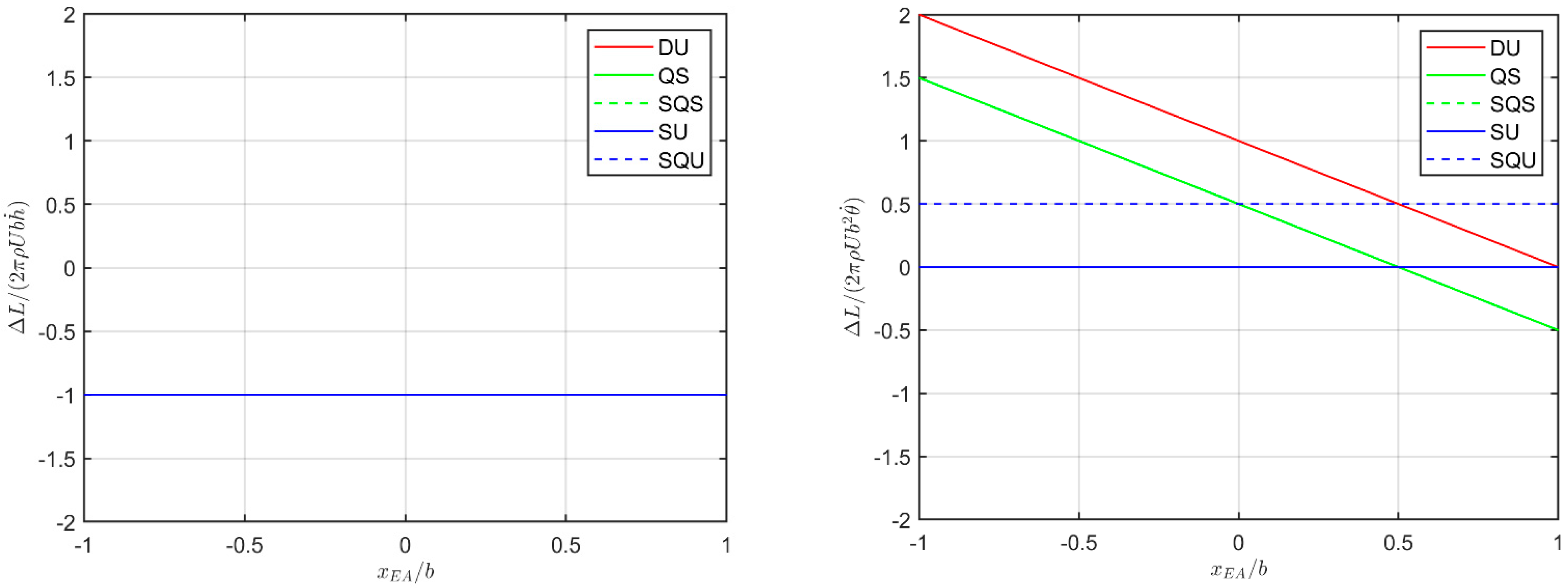
Recall that non-circulatory contributions involve but are not limited to apparent inertia effects, which are separately considered; of course, when the effective instantaneous angle of attack is given at the elastic axis, then it is uniform along the aerofoil’s chord and disregards contributions from the pitch rate. Figure 1 and Figure 2 then show the normalised coefficients of the aerodynamic damping terms for both lift and moment as a function of the elastic axis position along the aerofoil’s chord, as they both provide key insights on aeroelastic stability; of course, positive values are destabilising whereas negative ones are stabilising (with the total airload appearing on the right side of the aeroelastic equations). First of all, note that the plunge rate provides all approximations with the same effects: the lift derivative is independent of the position of the elastic axis and always stabilising, whereas the moment derivative decreases with moving the elastic axis backwards and becomes stabilising only when the latter is beyond the aerodynamic centre (i.e., the first quarter chord).
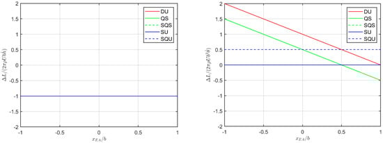
Figure 1.
Normalised aerodynamic damping derivatives for the aerofoil’s lift: plunge rate (left), pitch rate (right).
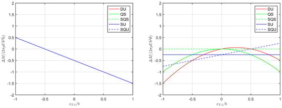
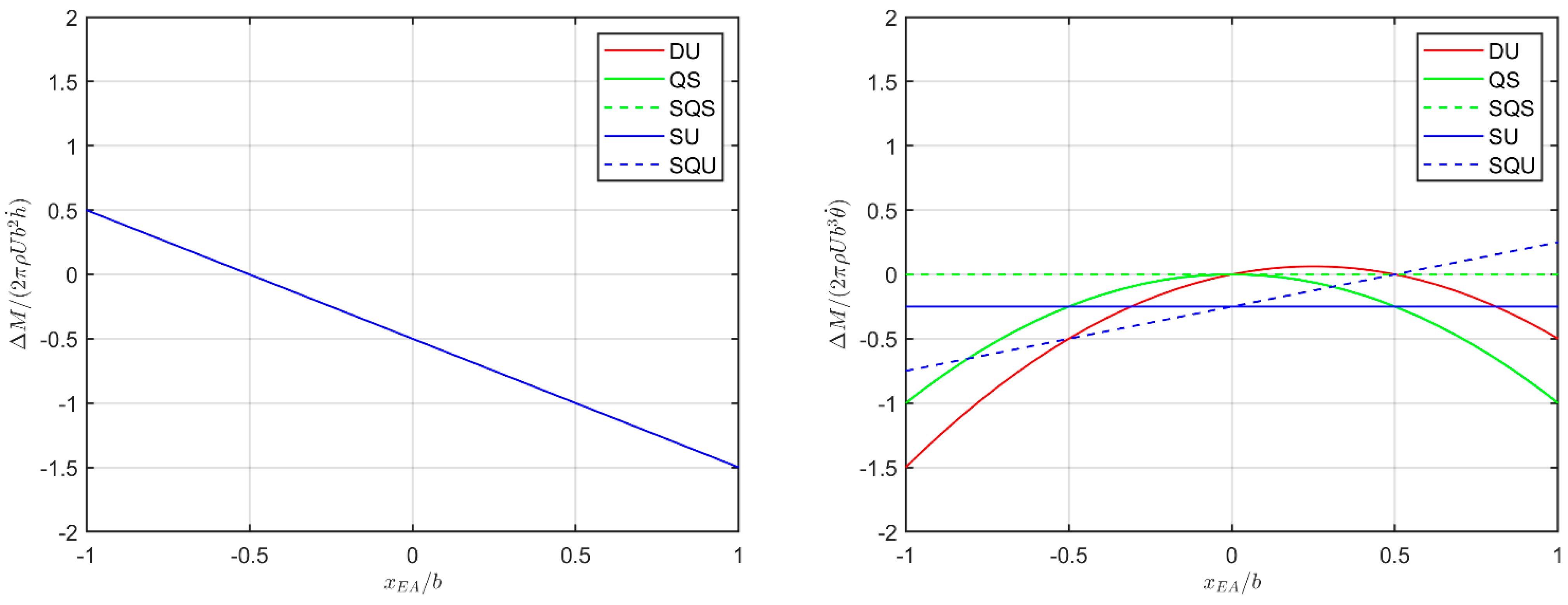
Figure 2.
Normalised aerodynamic damping derivatives for the aerofoil’s moment: plunge rate (left), pitch rate (right).
Variations in the characterisation of the aeroelastic stability of the typical section are then mostly driven by the pitch rate, the contribution of which differs among almost all aerodynamic models. In particular, the lift derivative of the DU model decreases with the elastic axis moving backwards but does remain always destabilising, whereas the moment derivative shows a parabolic dependence on the position of the elastic axis and is destabilising when the latter lies between the aerofoil’s mid-chord and control point (i.e., between the second and third quarter chord). Thus, this aerodynamic approximation gave controversial flutter results [4], since some cancellations between the circulatory and non-circulatory contributions to the unsteady airload do not hold in the absence of wake vorticity [15] and such inconsistencies can lead to very unrealistic results. The lift derivative of the QS model also decreases with the elastic axis moving backwards, but it becomes stabilising only when the latter lies beyond the aerofoil’s control point, whereas the moment derivative shows a parabolic dependence on the position of the elastic axis and is always stabilising but at the aerofoil’s mid-chord; however, this aerodynamic approximation also gave controversial flutter results [2]. The derivatives of the SQS model are always zero and thus do not contribute to the stability, which can lead to unrealistic results; the lift derivative of the SU model is also always zero, but the moment derivative is constant and always stabilising. Finally, the lift derivative of the SQU model is constant and always destabilising, whereas the moment derivative increases with the elastic axis moving backwards and becomes destabilized when the latter lies beyond the aerofoil’s control point (where SQU and DU models, as well as SU and QS models, are equivalent). The SQU aerodynamic approximation shall then not be used in such a case, which is, however, unlikely for practical application (due to both the geometrical features of real wings and static divergence issues in the first place).
Note that an iterative process where the value of these aerodynamic derivatives is refined based on successive flutter solutions was also proposed [9,80] (e.g., by updating the real part of Theodorsen’s function with a predictor-corrector scheme using the flutter reduced-frequency calculated at the last iteration, rather than just fixing the unitary value a priori). However, this approach is not considered here, since it is deemed ultimately inefficient in terms of computational cost when compared to that of the exact US model.
4. Flutter Analysis
From combining structural and aerodynamic models in vector-matrix form, the governing coupled ODEs become [2]:
where the structural inertia and stiffness matrices are constant, whereas the aerodynamic inertia, damping and stiffness matrices depend on the airload model adopted; as stated, two-dimensional, incompressible, inviscid flow is hereby assumed. With Laplace’s complex variable (where and relate to damping and frequency of the oscillations, respectively), the flutter instability may generally be investigated as [6]:
and the parametric aeroelastic stability boundary is obtained by monitoring the root locus as the reference airspeed increases in
the low-subsonic regime using the p-k method [88]. The latter is appropriate for lightly damped modes only, since structural dynamics and aerodynamic load are separately expressed in Laplace’s and Fourier’s domains, with s = iω on the flutter boundary (i.e., for resonant harmonic motion). When the airload is entirely expressed in the time domain only, the aeroelastic equations are formulated in the state space directly [10] and the continuation method [89] is particularly suitable; the characteristic equation for the flutter determinant is then a high-order polynomial in the reference airspeed, for which an exact quasi-steady solution exists at the flutter point [28].
In the absence of aerodynamic load, the coupled and uncoupled natural vibration frequencies are explicitly found as:
respectively, whereas retaining steady airload and
structural stiffness only results in the static aeroelastic divergence speed UD being [2]:
Note that the typical section has extensively been used to study and understand the flutter mechanism of flexible slender wings [90,91,92,93], both numerically [94,95] and experimentally [96,97]; steady and quasi-steady aerodynamics have been used to derive exact analytical solutions and grasp fundamental theoretical insights on the aeroelastic stability boundary [83,84,85]. In particular, such formulations grant a clear and complete overview of the problem at a conceptual level, which is essential for any engineering application, providing full control in terms of both results and their underlying assumptions. Although inherently limited, analytical approaches offer a wealth of qualitative information and quantitative details, as well as rigorous validation, for both educational and practical purposes [12,13]. As far as the p-k method is adopted for flutter analyses in the reduced frequency domain, all presented aerodynamic approximations lead to similar negligible computational cost with modern computers; however, unsteady and quasi-unsteady aerodynamics become more expensive as soon as added aerodynamic states are defined to write the unsteady airload in the time domain [18] within a state-space formulation (typically required to study the stability of nonlinear aeroelastic equations) where the p method can then be directly adopted for flutter analyses in Laplace’s domain [6]. Of course, the exact analytical expressions available for the stability boundary of linear aeroelastic equations within the lowest fidelity models come at no computational cost and ideal efficiency.
5. Results and Discussion
Numerical flutter test cases found in the literature for the typical section of a flexible wing are now analysed and clarified, specifying the input data and then critically assessing the influence of different aerodynamic approximations on the aeroelastic stability boundary, from both physical and mathematical perspectives. All relevant data are given in Table 2, where the position of elastic axis and gravity centre are expressed as the percentage of the aerofoil’s chord from the leading edge; incompressible flow is assumed in all cases with air density at sea level from the standard atmosphere [98]. Note that data for Case B [2] originally came from a previous book [8] where the centre of gravity (i.e., the static moment of inertia) is also stated incorrectly and has hence been amended here.
Table 2.
Aero-structural properties of test cases from the literature for flutter of a typical section in incompressible flow.
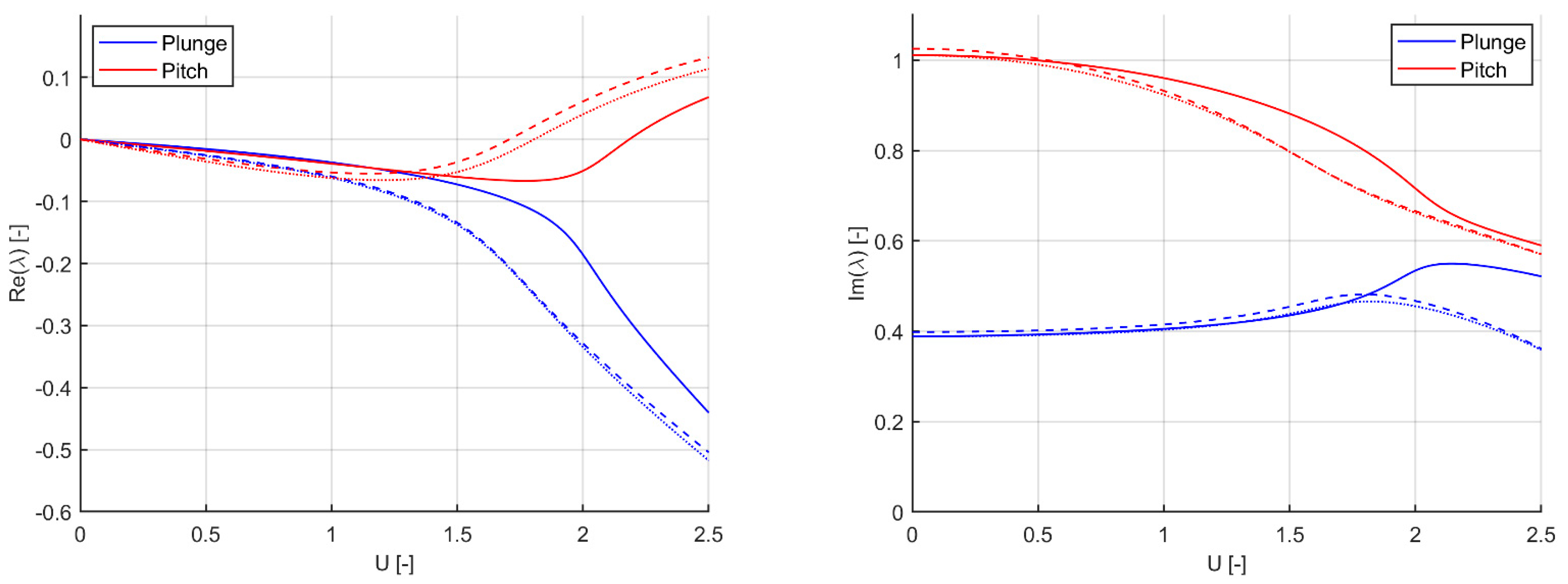
Flutter results for Case A [6] are given in Table 3; the related flutter diagrams for the evolution of the nondimensional complex eigenvalues are shown in Figure 3 and Figure 4, for selected aerodynamic models. In particular, the results from DU and SS models are not plotted since they are less relevant, as anticipated in the dedicated sections: those from the former model are questionable from a physical standpoint, while those from the latter model are already available in the references and provide no realistic evolution of modal damping.
Table 3.
Flutter analysis results for Case A using different aerodynamic models.
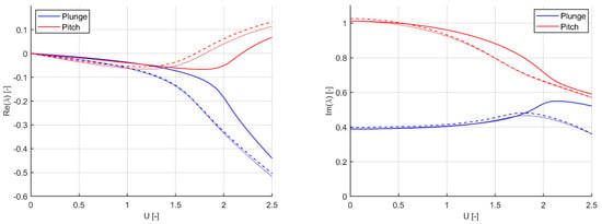
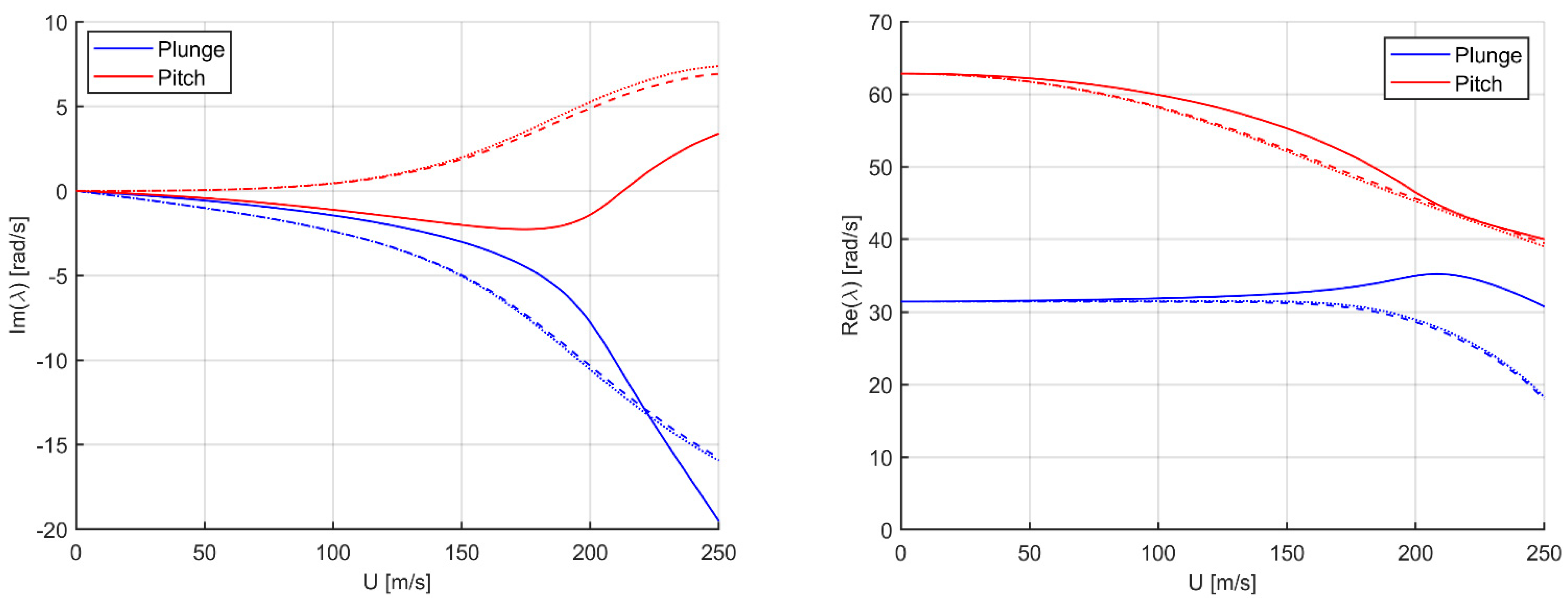
Figure 3.
Evolution of the complex eigenvalues for Case A: real part (left), imaginary part (right); continuous, dashed and dotted lines for US, SU and SQU aerodynamic models, respectively.
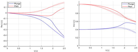
Figure 4.
Evolution of the complex eigenvalues for Case A: real part (left), imaginary part (right); continuous, dashed and dotted lines for QU, QS and SQS aerodynamic models, respectively.
With ωh = 0.398 rad/s and ωθ = 1.026 rad/s as the coupled natural vibration frequencies for the plunge and pitch modes, respectively, the static divergence speed is then found as UD = 2.83 m/s by all models, whereas the flutter speed varies considerably (note that these very low speeds satisfy the hypothesis of incompressible flow but are not meant to be practical per se, since they are only due to the convenient yet unrealistic choices of unitary semi-chord as well as uncoupled natural vibration frequency for the pitch mode). While flutter results from the QU and US models are rather close, all other aerodynamic approximations are quite conservative with respect to the latter but draw the same flutter mechanism, where the pitch modes become unstable and extract energy from the airflow through the plunge mode. Employing either the SU or SQU model leads to very similar flutter results, which are remarkably better than those obtained with the DU, SQS or QS model. This difference is confirmed by the evolution of the complex eigenvalues in the flutter diagrams (where the effect of the apparent flow inertia reducing the eigen-frequencies can be appreciated even at rest and the stability branches then depart progressively from the exact ones of the US model) and is exacerbated in the flutter reduced-frequency. Although quite higher than theoretically suitable for all quasi-steady aerodynamic models (especially for the QS one), the latter can still be used as a key indicator of the quality of the aerodynamic approximation with respect to the US model. The SS model is a special case though, as it provides a good approximation of the flutter point but brings no information about the evolution of the damping (which is essential to understand the evolution of the aeroelastic stability and run safe flight tests, for instance).
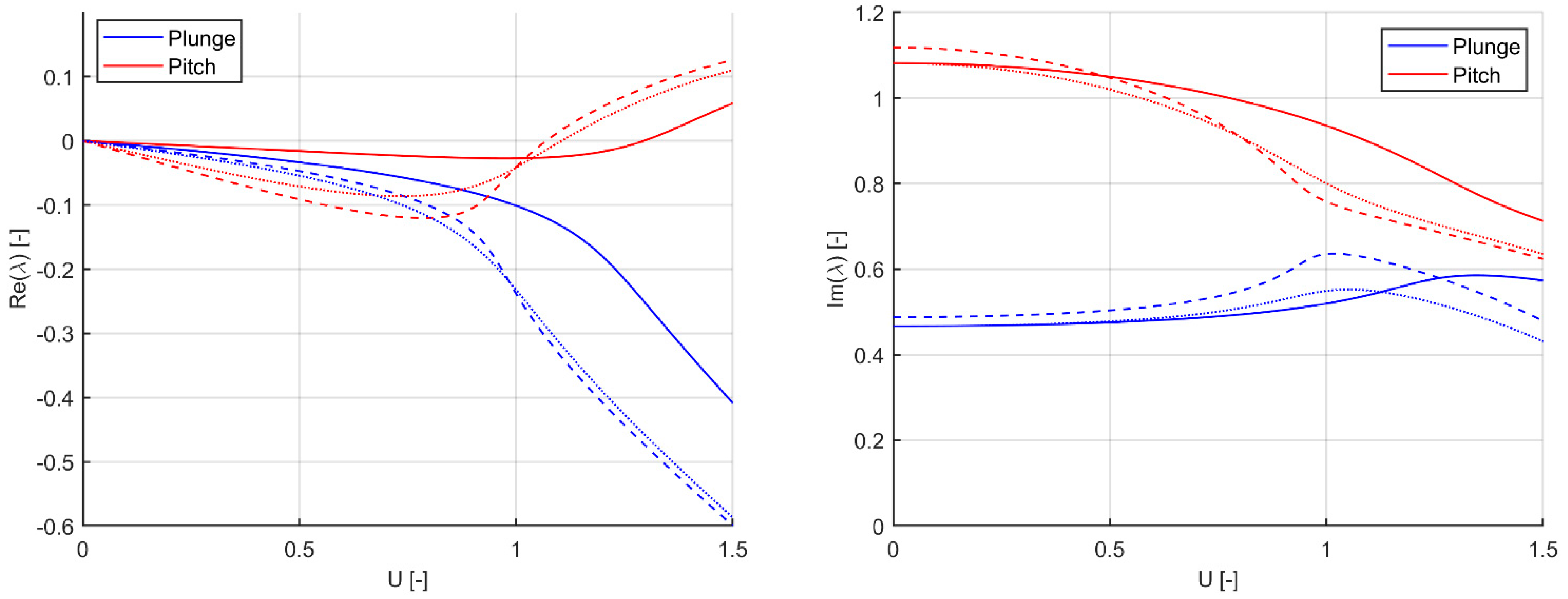
Flutter results for Case B [2] are given in Table 4; the related flutter diagrams for the evolution of the nondimensional complex eigenvalues are shown in Figure 5 and Figure 6 for the selected aerodynamic models. With ωh = 0.488 rad/s and ωθ = 1.118 rad/s, the coupled natural vibration frequencies for plunge and pitch modes, respectively, the static divergence speed is found as UD = 1.77 m/s by all models, while the flutter speed varies considerably (still, these very low speeds also satisfy the hypothesis of incompressible flow but are not meant to be any practical per se, since just due to the convenient yet unrealistic choices of unitary semi-chord as well as uncoupled natural vibration frequency for the pitch mode). The same general discussion as per Case A applies; nevertheless, it is worth stressing that the DU model is inherently unstable, the absence of apparent flow inertia lowers the flutter frequency calculated by the QU model significantly, whereas the SS model gives more conservative results than SU and SQU models.
Table 4.
Flutter analysis results for Case B using different aerodynamic models.
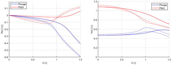
Figure 5.
Evolution of the complex eigenvalues for Case B: real part (left), imaginary part (right); continuous, dashed and dotted lines for US, SU and SQU aerodynamic models, respectively.
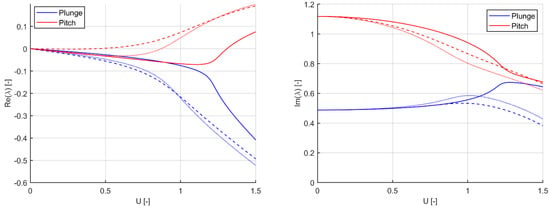
Figure 6.
Evolution of the complex eigenvalues for Case B: real part (left), imaginary part (right); continuous, dashed and dotted lines for QU, QS and SQS aerodynamic models, respectively.
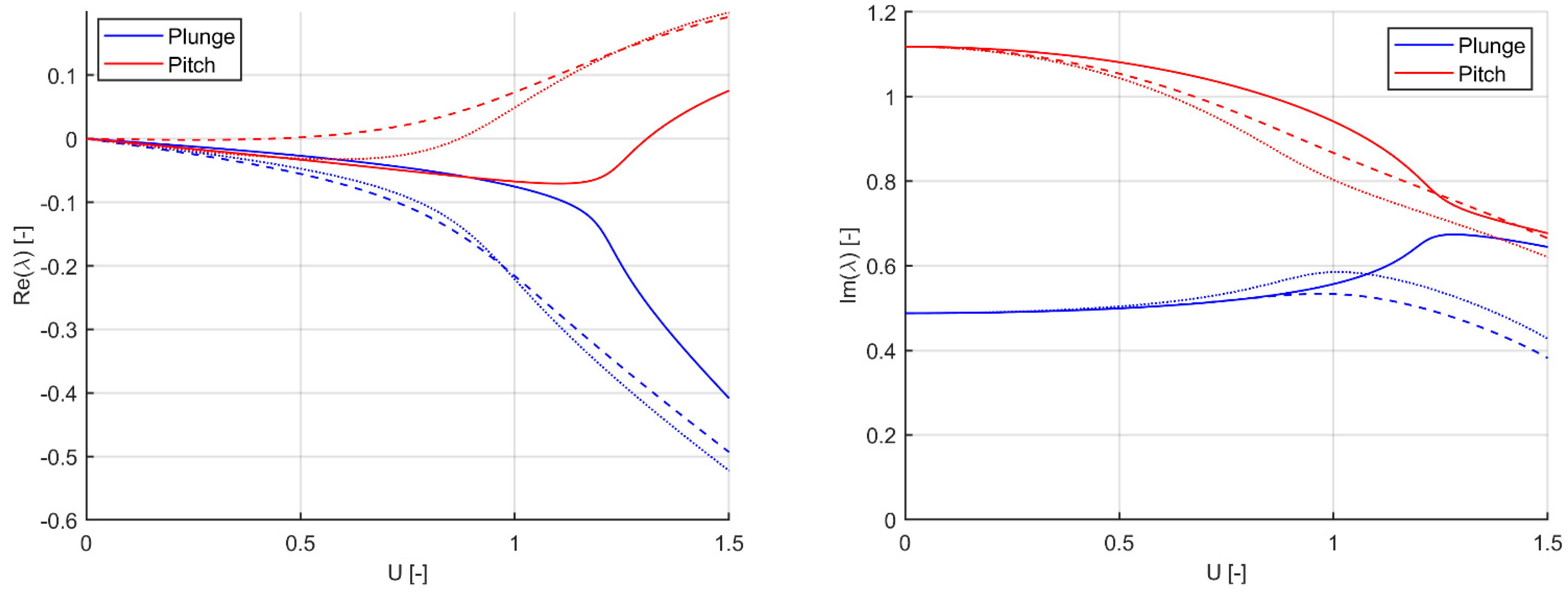
Flutter results for Case C [9] are given in Table 5; the related flutter diagrams for the evolution of the complex eigenvalues are shown in Figure 7 and Figure 8 for the selected aerodynamic models. The coupled natural vibration frequencies for plunge and pitch modes coincide with the uncoupled ones (since elastic axis and centre of gravity coincide), and the static divergence speed is found as UD = 261.5 m/s by all models, whereas the subsonic flutter speed varies considerably. The same general discussion as per Case A still applies; nevertheless, it is worth stressing that DU, QS and SQS models are inherently unstable, whereas the SS model finds no coalescence between plunge and pitch modes. Finally, Table 6 and Table 7 show a sensitivity analysis where the elastic axis is moved at the aerodynamic centre (where no static divergence occurs) and at the control point (where UD = 244.6 m/s), respectively. In the former case, a significant improvement is observed for the results obtained with all aerodynamic approximations (especially the SQS model) but the DU one; in the latter case, flutter would actually occur at a speed much higher than static divergence speed, but this is not foreseen by any quasi-steady approximation, as the DU and SQU models (which give same flutter results, as expected), as well as the QS and SQS models (which also give same flutter results, as expected), behave conservatively.
Table 5.
Flutter analysis results for Case C using different aerodynamic models; elastic axis at midchord.
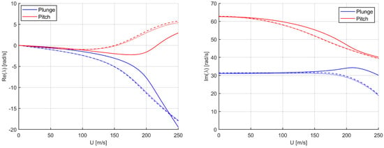
Figure 7.
Evolution of the complex eigenvalues for Case C: real part (left), imaginary part (right); continuous, dashed and dotted lines for US, SU and SQU aerodynamic models, respectively.
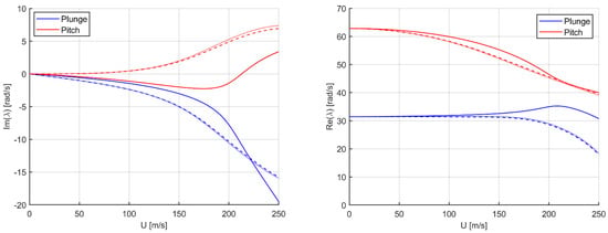
Figure 8.
Evolution of the complex eigenvalues for Case C: real part (left), imaginary part (right); continuous, dashed and dotted lines for QU, QS and SQS aerodynamic models, respectively.
Table 6.
Flutter analysis results for Case C using different aerodynamic models; elastic axis at aerodynamic centre.
Table 7.
Flutter analysis results for Case C using different aerodynamic models; elastic axis at control point.
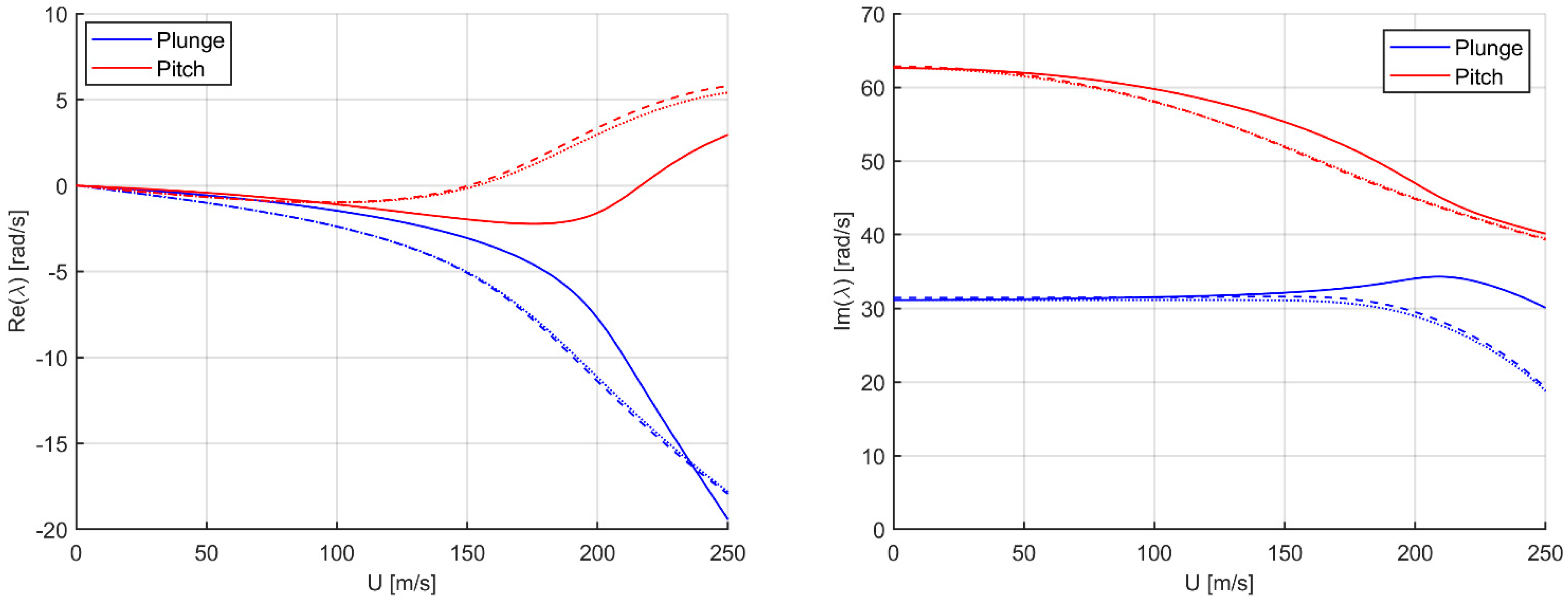
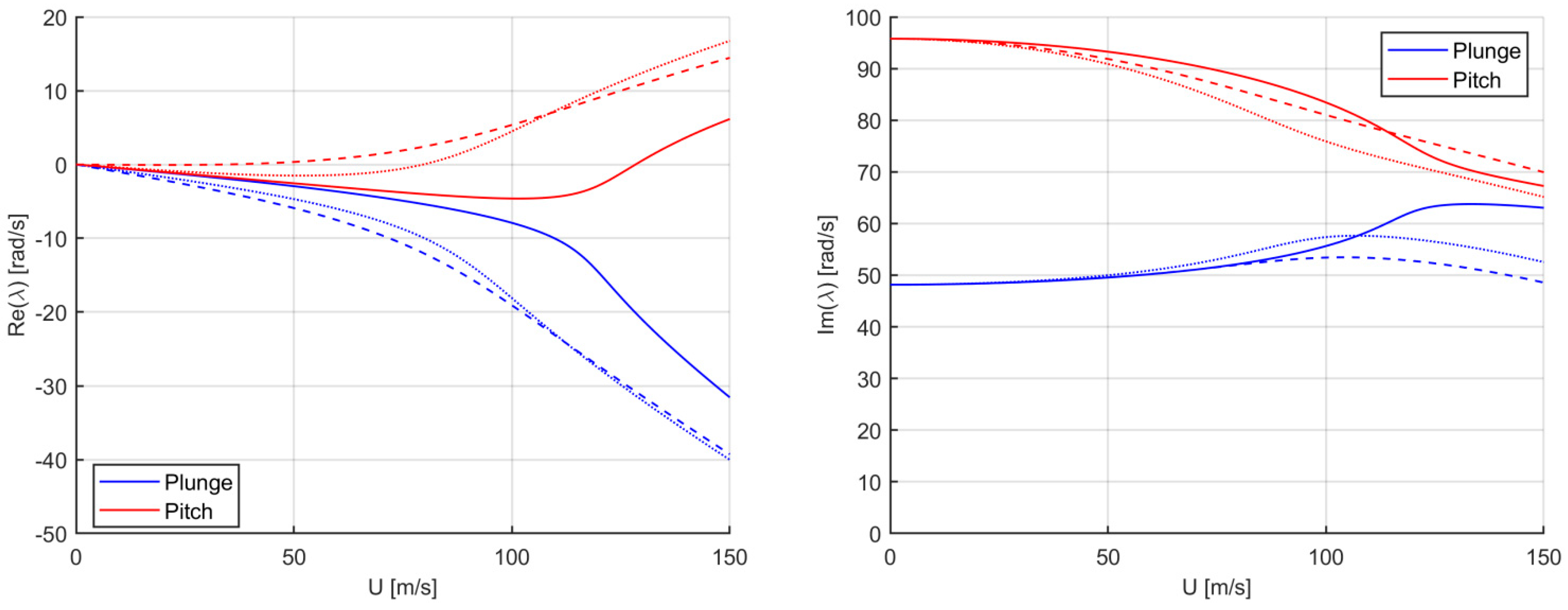
Within the proposed unified theoretical framework, the accuracy and robustness of all aerodynamic approximations presented have been assessed with respect to the exact unsteady theory for thin aerofoil. Goland’s wing [99,100] is now considered as a standard benchmark for validation and practical source of comparison with higher-fidelity data, since it has widely been used to assess many numerical methods and tools ranging from a Euler–Bernoulli beam coupled with unsteady [101] or quasi-steady [86] aerodynamics, an intrinsic beam formulation coupled with inflow theory [102,103], a beam-based finite element model coupled with doublet lattice [104] or unsteady vortex lattice [104,105], or boundary element [87] aerodynamics. It is a uniform, thin, flat, rectangular and cantilevered wing with its root clamped at its elastic axis; the properties of its typical section idealisation are given in Table 8. The wing is aligned with the horizontal freestream and exhibits the prototypical flutter mechanism coupling its fundamental bending and torsion modes, with the latter becoming unstable and extracting energy from the airstream through the former. Assuming standard atmosphere at sea level [98] and multiplying the off-diagonal terms of all aero-structural matrices by the modal cross-projection factor r ≈ 0.959 [6,87], Table 9 and Figure 9 and Figure 10 show the flutter results for all aerodynamic approximations. With ωh = 48.16 rad/s and ωθ = 95.78 rad/s, the coupled natural vibration frequencies for the plunge and pitch modes, respectively, the static divergence speed is readily found as UD = 252.3 m/s by all models whereas the flutter speed varies considerably, as expected. In particular, the present results for the US model are in perfect agreement with those already found in the literature for two-dimensional flow [99,100,101,102,103], providing full higher-fidelity validation as well as confirming the assumption of incompressible fluid at low speeds [7]. Note that the present results for DU and QS models are also in exact agreement with higher-fidelity ones based on a Euler–Bernoulli beam model [86], granting further validation as well as confirming the typical section concept is suitable for flutter analysis of slender wings in subsonic flow when their aero-structural properties are rather homogeneous and their natural vibration modes are well separated [13].
Table 8.
Aero-structural properties for the typical section of Goland’s wing in incompressible flow.
Table 9.
Flutter analysis results for Goland’s wing using different aerodynamic models.
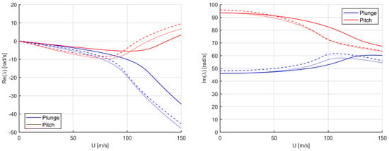
Figure 9.
Evolution of the complex eigenvalues for Goland’s wing: real part (left), imaginary part (right); continuous, dashed and dotted lines for US, SU and SQU aerodynamic models, respectively.
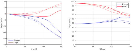
Figure 10.
Evolution of the complex eigenvalues for Goland’s wing: real part (left), imaginary part (right); continuous, dashed and dotted lines for QU, QS and SQS aerodynamic models, respectively.
The numerical assessment revealed that the accuracy of all aerodynamic approximations for flutter analysis is highly dependent on the aero-structural configuration of the typical section [83,84,85]; this is true for the QU model too, whenever apparent flow inertia effects are predominant. However, SU and SQU models were demonstrated to be quite robust in providing reliable flutter analyses when the elastic axis lay ahead of the aerofoil’s control point and flutter occurs before static divergence, as is typical in practice [8,9]. As for the computational cost, lower-fidelity semi-analytical solutions are almost instantaneous and demand minimal pre- and post-processing (if any at all), while providing an enhanced theoretical understanding; therefore, they enable efficient multidisciplinary exploration of a large design variable space for innovative aircraft concepts and configurations [12,13]. Note that further numerical savings may be obtained by exploiting efficient tuning techniques and surrogate models [106,107] with the effective synthesis of problem complexity.
6. Conclusions
Different analytical formulations for the time-dependent aerodynamic load of a thin aerofoil have been reviewed in this work and numerical flutter results available in the literature for the typical section of a flexible wing have hence been clarified; inviscid, two-dimensional, incompressible, potential flow is considered in all test cases. The latter have been investigated using exact theory for small airflow perturbations, complemented by p-k flutter analysis. Starting from unsteady aerodynamics and ending with steady aerodynamics, quasi-unsteady and quasi-steady aerodynamic models have been systematically derived by successive simplifications within a unified vorticity-based approach, where the circulatory or non-circulatory nature of all effects can explicitly be identified and the physical meaning of all terms can fully be traced. Thus, the proposed theoretical framework allows drawing practical guidelines for the most appropriate use of all aerodynamic approximations. Special focus has been devoted to the aerodynamic damping terms as a function of the elastic axis position along the aerofoil’s chord in the analytical expressions of lift and moment, and they have been shown to provide key insights on the aeroelastic stability, especially through the role of the pitch rate. In particular, the derivatives of the simplified quasi-steady model with respect to the latter are always zero and thus do not contribute to the aeroelastic stability, which can lead to unreliable flutter results; the lift derivative of the simplified unsteady model is also always zero, but the moment derivative is constant and always stabilising. In addition, note that including the time rate of the circulatory vorticity in the absence of wake vorticity provides the aerofoil with an unphysically loaded trailing edge as a stagnation point.
The non-circulatory contributions involve but are not limited to apparent flow inertia effects: while the former have been found essential for a reliable representation of both aeroelastic stability root locus and flutter mechanism, the latter tend to lower the flutter frequency and become important in the presence of light damping. Neglecting the wake’s inflow eliminates lag effects on the circulatory flow around the aerofoil due to feedback from the shed vorticity (governed by Kutta’s condition at the unloaded trailing edge) and thus avoids an inconvenient formulation for the unsteady airload in both time and frequency domains. However, some cancellations between circulatory and non-circulatory contributions do not occur anymore: a degenerate model results that is inherently inconsistent as well as unstable when the elastic axis lies between the aerofoil’s mid-chord and its control point (i.e., between the second and third quarter chord) and often gives controversial flutter results otherwise. It has also been found that higher complexity does not imply higher accuracy and generality, depending on the specific application. In particular, the plunge rate provides all approximations with the same effects: the lift derivative is independent of the position of the elastic axis and always stabilising, while the moment derivative decreases with the elastic axis moving backward and becomes stabilised only when the latter is beyond the aerodynamic centre (i.e., the first quarter chord). Thus, the aeroelastic stability of a typical section is mostly characterised by the pitch rate, the contribution of which differs among almost all aerodynamic models. Disregarding the pitch rate in the effective instantaneous angle of attack makes the latter uniform along the aerofoil’s chord and avoids inconvenient singularities, which tend to trigger unphysical behaviours for harmonic motion at low reduced frequency: this choice was found to provide the typical section with a more realistic aeroelastic stability boundary even beyond the hypothesis of quasi-steady flow, especially when either the simplified unsteady or simplified quasi-unsteady aerodynamic model is employed.
The latter aerodynamic approximations are hence suggested for robust estimations of the aeroelastic response of a flexible wing in practical cases, whenever the elastic axis lies ahead of the control point (i.e., the third quarter chord): they both feature a stabilising couple proportional to the pitch rate, but the simplified quasi-unsteady model also embeds apparent flow inertia effects (which are important, as some non-circulatory effects were found to be induced by the wake’s vorticity within the exact unsteady model). However, within a rigorous assessment from both physical and mathematical perspectives supported by comprehensive numerical results and sensitivity analyses, their accuracy for flutter analysis is still found to be dependent on the specific aero-structural configuration, even when the airflow is actually quasi-steady with small aerofoil’s oscillations at a very low reduced frequency.
Funding
This research received no external funding.
Conflicts of Interest
The author declares no conflict of interest.
Nomenclature
| aerofoil semi-chord | |
| aerofoil chord | |
| Theodorsen’s lift-deficiency function | |
| sectional lift derivative with respect to angle of attack | |
| , | aerodynamic and structural damping matrices |
| sectional plunge displacement (positive upwards) | |
| Hankel’s function of n-th order and m-th kind | |
| , | reduced frequency of aerofoil oscillations and flutter |
| , | stiffness of vertical/flexural and angular/torsional springs |
| , | aerodynamic and structural stiffness matrices |
| sectional aerodynamic lift (positive upwards) | |
| sectional mass per unit span | |
| sectional aerodynamic moment (positive clockwise) | |
| , | aerodynamic and structural stiffness matrices |
| sectional net pressure airload along the aerofoil | |
| aerodynamic load matrix | |
| Laplace’s complex variable | |
| physical time | |
| Chebyshev’s polynomials | |
| , | horizontal flow velocity (flow perturbation) |
| horizontal reference airspeeds | |
| , | flutter and divergence airspeeds |
| vertical aerofoil velocity (flow perturbation) | |
| , | vertical flow velocity and wake’s inflow (flow perturbation) |
| vertical velocity of aerofoil’s control point | |
| , | longitudinal coordinates from aerofoil’s mid-chord (positive aft) |
| , | longitudinal coordinates of the sectional centre of gravity and elastic axis |
| aerofoil’s vertical displacement | |
| , | instantaneous effective angle of attack and Glauert’s coefficients |
| , , | global, aerofoil and wake vorticity distributions |
| , , | global, aerofoil and wake vorticity circulations |
| normalised longitudinal coordinate from aerofoil’s mid-chord (positive aft) | |
| sectional pitch displacement (positive clockwise) | |
| , | sectional mass moments of inertia at centre of gravity and elastic axis |
| air density | |
| damping of aerofoil oscillations (real Laplace variable) | |
| , | reduced time |
| , | fluid potential function (flow perturbation) |
| Wagner’s indicial lift function | |
| Glauert’s angle along aerofoil chord | |
| , | frequencies of aerofoil oscillations and flutter (imaginary Laplace variable) |
| , | natural frequencies of sectional plunge and pitch modes |
| , | quasi-steady and unsteady contributions (for any aerodynamic quantity) |
| , | circulatory and non-circulatory contributions (for any aerodynamic quantity) |
Appendix A
The overall analytical strategy for modelling unsteady aerodynamic loads may be summarised as follows. Adopting a vorticity-based approach for the incompressible potential flow around a thin rigid aerofoil [1,32], the horizontal component of the instantaneous perturbation velocity is found to be directly proportional to the local vorticity along the latter [4], whereas the vertical component is given by Hilbert’s formula and must satisfy both Neumann’s and Kutta–Joukowski’s conditions for inviscid irrotational flow [3,4]. While Dirichlet’s boundary condition for the asymptotic airflow is inherently embedded in the freestream [7], Neumann’s impermeability boundary condition imposes the airflow as always tangential to aerofoil’s mean line [14]. Kutta’s and Joukowski’s theorems [39,40] establish the resultant aerodynamic force as being normal to freestream and proportional to circulation, as the airflow leaves the aerofoil’s trailing edge smoothly with finite speed [7,15]. While Kutta’s condition enforces physical consistence without flow singularity at the trailing edge [16,17], Bernoulli’s unsteady linearised equation [4,14] provides the net pressure airload acting across upper and lower surfaces of the aerofoil. Finally, the aerodynamic lift and moment are obtained by integrating such pressure airload as an explicit function of the aerofoil’s kinematic [5,10].
In particular, for a flat aerofoil the vertical perturbation velocity may alternatively be expressed using the aerofoil’s impermeability condition and Glauert’s expansion as [7]:
where the latter are Chebyshev’s polynomials of the first kind [32,43], with ; these are consistent with a generalised form of the unsteady bound vorticity and circulation that satisfy Kutta’s condition at the aerofoil’s trailing edge, namely [7]:
and can eventually be integrated to give the unsteady airload in terms of Glauert’s coefficients directly, which include the wake’s inflow [5,33]. Note that this model was recently generalised for a thin aerofoil with morphing camber [36,37,38,43].
However, when the wake’s inflow is marginal, the solution is solely driven by the aerofoil’s kinematics as [7]:
and the vorticity distribution along the aerofoil’s chord reduces to:
which coincides with the expression found by thin aerofoil theory [15,36] and provides the aerofoil’s trailing edge with a stagnation point (i.e., regardless of the motion of the typical section). After integration of the pressure distribution [7]:
the total lift and moment around the elastic axis read:
however, note that the aerofoil’s trailing edge is loaded unless the rate of change of the bound circulation is marginal. It is also worth stressing that the bound circulation is indeed proportional to the airfoil’s instantaneous kinematics at the control point, as per an equivalent lumped-vortex model in steady airflow [30] where the counter-rotating wake vortex is infinitely far behind the aerofoil.
When all apparent inertia terms are also negligible, the pressure distribution grants an unloaded trailing edge and the aerofoil’s quasi-steady airload simplifies to [28]:
where the rate of change of the bound circulation is also disregarded.
References
- Jones, R.T. Classical Aerodynamic Theory; NASA-RP-1050; NASA: Washington, DC, USA, 1979.
- Dowell, E.H. A Modern Course in Aeroelasticity; Springer: Berlin/Heidelberg, Germany, 2004. [Google Scholar]
- Gulcat, U. Fundamentals of Modern Unsteady Aerodynamics; Springer: Berlin/Heidelberg, Germany, 2011. [Google Scholar]
- Bisplinghoff, R.L.; Ashley, H.; Halfman, R.L. Aeroelasticity; Dover: Mineola, NY, USA, 1996. [Google Scholar]
- Peters, D.A. Two-Dimensional Incompressible Unsteady Airfoil Theory–A Review. J. Fluids Struct. 2008, 24, 295–312. [Google Scholar] [CrossRef]
- Hodges, D.; Pierce, G. Introduction to Structural Dynamics and Aeroelasticity; Cambridge University Press: Cambridge, UK, 2002. [Google Scholar]
- Katz, J.; Plotkin, A. Low-Speed Aerodynamics; Cambridge University Press: Cambridge, UK, 2001. [Google Scholar]
- Bisplinghoff, R.L.; Ashley, H. Principles of Aeroelasticity; Dover: Mineola, NY, USA, 2013. [Google Scholar]
- Wright, J.R.; Cooper, J.E. Introduction to Aircraft Aeroelasticity and Loads; Wiley: Hoboken, NJ, USA, 2014. [Google Scholar]
- Leishman, J.G. Principles of Helicopter Aerodynamics; Cambridge University Press: Cambridge, UK, 2006. [Google Scholar]
- Berci, M. Semi-analytical static aeroelastic analysis and response of flexible subsonic wings. Appl. Math. Comput. 2015, 267, 148–169. [Google Scholar] [CrossRef]
- Berci, M.; Cavallaro, R. A Hybrid Reduced-Order Model for the Aeroelastic Analysis of Flexible Subsonic Wings—A Parametric Assessment. Aerospace 2018, 5, 76. [Google Scholar] [CrossRef] [Green Version]
- Berci, M.; Torrigiani, F. Multifidelity Sensitivity Study of Subsonic Wing Flutter for Hybrid Approaches in Aircraft Multidisciplinary Design and Optimisation. Aerospace 2020, 7, 161. [Google Scholar] [CrossRef]
- Newman, J.N. Marine Hydrodynamics; MIT Press: Cambridge, MA, USA, 1977. [Google Scholar]
- Epps, B.P.; Roesler, B.T. Vortex Sheet Strength in the Sears, Küssner, Theodorsen, and Wagner Aerodynamics Problems. AIAA J. 2018, 56, 889–904. [Google Scholar] [CrossRef]
- Theodorsen, T. General Theory of Aerodynamic Instability and the Mechanism of Flutter; NACA-TR-496; NACA: Washington, DC, USA, 1935. [Google Scholar]
- Wagner, H. Uber die Entstenhung des Dynamischen Auftriebes von Tragflugeln. Z. Angew. Math. und Mech. 1925, 5, 17–35. [Google Scholar] [CrossRef] [Green Version]
- Dimitriadis, G. Introduction to Nonlinear Aeroelasticity; Wiley: Hoboken, NJ, USA, 2017. [Google Scholar]
- Dennis, S.T. Undergraduate Aeroelasticity: The Typical Section Idealization Re-Examined. Int. J. Mech. Eng. Educ. 2013, 41, 72–91. [Google Scholar] [CrossRef]
- Weisshaar, T.A. Static and Dynamic Aeroelasticity. In Encyclopedia of Aerospace Engineering; Wiley: Hoboken, NJ, USA, 2010. [Google Scholar]
- Quarteroni, A.; Rozza, G. Reduced Order Methods for Modeling and Computational Reduction; Springer International Publishing: Cham, Switzerland, 2014. [Google Scholar]
- Qu, Z.Q. Model. Order Reduction Techniques with Applications in Finite Element Analysis; Springer: Berlin/Heidelberg, Germany, 2004. [Google Scholar]
- Silva, W.A. AEROM: NASA’s Unsteady Aerodynamic and Aeroelastic Reduced-Order Modeling Software. Aerospace 2018, 5, 41. [Google Scholar] [CrossRef] [Green Version]
- Theodorsen, T.; Garrick, L.E. Flutter Calculations in Three Degrees of Freedom; NACA-TR-741; NASA: Washington, DC, USA, 1942.
- Theodorsen, T.; Garrick, L.E. Nonstationary Flow about a Wing-Aileron-Tab Combination Including Aerodynamic Balance; NACA-736; NASA: Washington, DC, USA, 1942.
- Zeiler, T.A. Results of Theodorsen and Garrick Revisited. J. Aircr. 2000, 37, 918–920. [Google Scholar] [CrossRef]
- Kussner, H.G.; Schwartz, I. The Oscillating Wing with Aerodynamically Balanced Elevator; NACA-TM-991; NASA: Washington, DC, USA, 1941.
- Fung, Y.C. An Introduction to the Theory of Aeroelasticity; Dover: Mineola, NY, USA, 1993. [Google Scholar]
- Yang, B. Strain, Stress and Structural Dynamics; Elsevier: Amsterdam, The Netherlands, 2005. [Google Scholar]
- Karamcheti, K. Principles of Ideal-Fluid Aerodynamics; Wiley: New York, NY, USA, 1967. [Google Scholar]
- Prandtl, L. Applications of Modern Hydrodynamics to Aeronautics; NACA-TR-116; NASA: Washington, DC, USA, 1921.
- Glauert, H. The Elements of Aerofoil and Airscrew Theory; Cambridge University Press: Cambridge, UK, 1983. [Google Scholar]
- Von Karman, T.; Sears, W.R. Airfoil Theory for Non-Uniform Motion. J. Aeronaut. Sci. 1938, 5, 379–390. [Google Scholar] [CrossRef]
- Jones, R.T. The Unsteady Lift of a Wing of Finite Aspect Ratio; NACA-TR-681; NASA: Washington, DC, USA, 1940.
- Anderson, J.D. Fundamentals of Aerodynamics; McGraw-Hill: New York, NY, USA, 2017. [Google Scholar]
- Johnston, C.O. Review, Extension and Application of Unsteady Thin Airfoil Theory; CIMSS-04-101; CIMSS: Madison, WI, USA, 2004. [Google Scholar]
- Johnston, C.O.; Mason, W.H.; Han, C. Unsteady thin airfoil theory revisited for a general deforming airfoil. J. Mech. Sci. Technol. 2010, 24, 2451–2460. [Google Scholar] [CrossRef]
- Gaunaa, M. Unsteady 2D Potential-Flow Forces on a Thin Variable Geometry Airfoil Undergoing Arbitrary Motion; Risø–R–1478; Risø: Roskilde, Denmark, 2006. [Google Scholar]
- Kutta, W.M. Auftriebskräfte in Strömenden Flüssigkeiten. Illus. Aeronaut. Mitt. 1902, 6, 133–135. [Google Scholar]
- Joukowski, N.E. Sur les Tourbillons Adjionts. Traraux Sect. Phys. Soc. Imp. Amis Sci. Nat. 1906, 13, 261–284. [Google Scholar]
- Bungartz, H.J.; Schafer, M. Fluid-Structure Interaction: Modelling, Simulation, Optimization; Springer: Berlin/Heidelberg, Germany, 2006. [Google Scholar]
- Neumark, S. Vortex Pressure Distribution on an Airfoil in Nonuniform Motion. J. Aeronaut. Sci. 1952, 19, 214–215. [Google Scholar] [CrossRef]
- Peters, D.A.; Hsieh, M.-C.A.; Torrero, A. A State-Space Airloads Theory for Flexible Airfoils. J. Am. Helicopter Soc. 2007, 52, 329–342. [Google Scholar] [CrossRef]
- Queijo, M.J.; Wells, W.R.; Keskar, D.A. Approximate Indicial Lift Function for Tapered, Swept Wings in Incompressible Flow; NASA-TP-1241; NASA: Washington, DC, USA, 1978.
- Berci, M.; Righi, M. An enhanced analytical method for the subsonic indicial lift of two-dimensional aerofoils–with numerical cross-validation. Aerosp. Sci. Technol. 2017, 67, 354–365. [Google Scholar] [CrossRef]
- Righi, M.; Berci, M. On Elliptical Wings in Subsonic Flow: Indicial Lift Generation via CFD Simulations-with Parametric Analytical Approximations. ASD J. 2019, 7, 1–17. [Google Scholar]
- Ronch, A.D.A.; Ventura, A.; Righi, M.; Franciolini, M.; Berci, M.; Kharlamov, D. Extension of analytical indicial aerodynamics to generic trapezoidal wings in subsonic flow. Chin. J. Aeronaut. 2018, 31, 617–631. [Google Scholar] [CrossRef]
- Jones, W.P. Aerodynamic Forces on Wings in Non-Uniform Motion; ARC-R&M-2117; ARC: London, UK, 1945. [Google Scholar]
- Berci, M. Lift-Deficiency Functions of Elliptical Wings in Incompressible Potential Flow: Jones’ Theory Revisited. J. Aircr. 2016, 53, 599–602, Erratum in 2017, 54, 1–2. [Google Scholar] [CrossRef]
- Boutet, J.; Dimitriadis, G. Unsteady Lifting Line Theory Using the Wagner Function for the Aerodynamic and Aeroelastic Modeling of 3D Wings. Aerospace 2018, 5, 92. [Google Scholar] [CrossRef] [Green Version]
- Sears, W.R. Operational methods in the theory of airfoils in non-uniform motion. J. Frankl. Inst. 1940, 230, 95–111. [Google Scholar] [CrossRef]
- Vepa, R. Finite State Modeling of Aeroelastic Systems; NASA-CR-2779; NASA: Washington, DC, USA, 1977.
- Berci, M.; Dimitriadis, G. A combined Multiple Time Scales and Harmonic Balance approach for the transient and steady-state response of nonlinear aeroelastic systems. J. Fluids Struct. 2018, 80, 132–144. [Google Scholar] [CrossRef]
- Reissner, E. On the General Theory of Thin Airfoils for Non-Uniform Motion; NACA-TN-946; NASA: Washington, DC, USA, 1944.
- Radok, J.R.M. The Theory of Aerofoils in Unsteady Motion. Aeronaut. Q. 1952, 3, 297–320. [Google Scholar] [CrossRef]
- Van De Vooren, A.I. Unsteady Aerofoil Theory. Adv. Appl. Mech. 1958, 5, 35–89. [Google Scholar]
- Perry, B. Comparison of Theodorsen’s Unsteady Aerodynamic Forces with Doublet Lattice Generalized Aerodynamic Forces; NASA/TM–2017-219667; NASA: Washington, DC, USA, 2017.
- Mateescu, D.; Abdo, M. Theoretical Solutions for Unsteady Flows Past Oscillating Flexible Airfoils Using Velocity Singularities. J. Aircr. 2003, 40, 153–163. [Google Scholar] [CrossRef]
- Berci, M.; Gaskell, P.H.; Hewson, R.W.; Toropov, V.V. A semi-analytical model for the combined aeroelastic behaviour and gust response of a flexible aerofoil. J. Fluids Struct. 2013, 38, 3–21. [Google Scholar] [CrossRef]
- Kemp, N.H.; Homicz, G. Approximate unsteady thin-airfoil theory for subsonic flow. AIAA J. 1976, 14, 1083–1089. [Google Scholar] [CrossRef]
- Mateescu, D. Theoretical Solutions for Unsteady Compressible Subsonic Flows Past Oscillating Rigid and Flexible Airfoils. Math. Eng. Sci. Aerosp. 2011, 2, 1–27. [Google Scholar]
- Hewson-Browne, R.C. The Oscillation of a Thick Aerofoil in an Incompressible Flow. Q. J. Mech. Appl. Math. 1963, 16, 79–92. [Google Scholar] [CrossRef]
- Woods, L.C. The Lift and Moment Acting on a Thick Aerofoil in Unsteady Motion. Philosophical Transactions of the Royal Soci-ety of London-Series, A. Math. Phys. Sci. 1954, 247, 131–162. [Google Scholar]
- Giesing, J.P. Nonlinear two-dimensional unsteady potential flow with lift. J. Aircr. 1968, 5, 135–143. [Google Scholar] [CrossRef]
- Riso, C.; Riccardi, G.; Mastroddi, F. Semi-analytical unsteady aerodynamic model of a flexible thin airfoil. J. Fluids Struct. 2018, 80, 288–315. [Google Scholar] [CrossRef]
- Liu, T.; Wang, S.; Zhang, X.; He, G. Unsteady Thin-Airfoil Theory Revisited: Application of a Simple Lift Formula. AIAA J. 2015, 53, 1492–1502. [Google Scholar] [CrossRef]
- Ericsson, L.E.; Reding, J.P. Unsteady Airfoil Stall, Review and Extension. J. Aircr. 1971, 8, 609–616. [Google Scholar] [CrossRef]
- Ahaus, L. An Airloads Theory for Morphing Airfoils in Dynamic Stall with Experimental Correlation; Washington University in St. Louis: St. Louis, MO, USA, 2010. [Google Scholar]
- Hoblit, F.M. Gust Loads on Aircraft: Concepts and Applications; American Institute of Aeronautics and Astronautics (AIAA): Reston, VA, USA, 1988. [Google Scholar]
- Kussner, H.G. Zusammenfassender Beritch uber den Instationaren Auftrieb von Flugeln. Luftfahrtforsch 1936, 13, 410–424. [Google Scholar]
- Kayran, A. Kussner’s Function in the Sharp Edged Gust Problem–A Correction. J. Aircr. 2006, 43, 1596–1599. [Google Scholar] [CrossRef]
- Jones, A.R.; Cetiner, O. Overview of Unsteady Aerodynamic Response of Rigid Wings in Gust Encounters. AIAA J. 2021, 59, 731–736. [Google Scholar] [CrossRef]
- Garrick, L.E. On Some Reciprocal Relations in the Theory of Nonstationary Flows; NACA-TR-629; NASA: Washington, DC, USA, 1938.
- Sears, W.R.; Kuethe, A.M. The Growth of the Circulation of an Airfoil Flying through a Gust. J. Aeronaut. Sci. 1939, 6, 376–378. [Google Scholar] [CrossRef]
- Pratt, K.G. A Revised Formula for the Calculation of Gust Loads; NACA-TN-2964; NASA: Washington, DC, USA, 1953.
- Basu, B.C.; Hancock, G.J. The unsteady motion of a two-dimensional aerofoil in incompressible inviscid flow. J. Fluid Mech. 1978, 87, 159–178. [Google Scholar] [CrossRef]
- Berci, M.; Mascetti, S.; Incognito, A.; Gaskell, P.H.; Toropov, V.V. Dynamic Response of Typical Section Using Variable-Fidelity Fluid Dynamics and Gust-Modeling Ap-proaches–With Correction Methods. J. Aerosp. Eng. 2014, 27, 1–24. [Google Scholar] [CrossRef]
- Zimmerman, N.H.; Weissenburger, J.T. Prediction of flutter onset speed based on flight testing at subcritical speeds. J. Aircr. 1964, 1, 190–202. [Google Scholar] [CrossRef]
- Rodden, W.P. Theoretical and Computational Aeroelasticity; Crest Publishing: Los Angeles, CA, USA, 2011. [Google Scholar]
- Hancock, G.J.; Wright, J.R.; Simpson, A. On the Teaching of the Principles of Wing Flexure-Torsion Flutter. Aeronaut. J. 1985, 89, 285–305. [Google Scholar]
- Miles, J.W. Quasi-stationary airfoil theory. J. Aeronaut. Sci. 1949, 16, 440. [Google Scholar]
- Miles, J.W. Quasi-stationary airfoil theory in subsonic compressible flow. J. Aeronaut. Sci. 1949, 16, 509. [Google Scholar] [CrossRef] [Green Version]
- Goland, M. The Quasi-Steady Air Forces for Use in Low-Frequency Stability Calculations. J. Aeronaut. Sci. 1950, 17, 601–608. [Google Scholar] [CrossRef]
- Dugundji, J. Effect of Quasi-Steady Air Forces on Incompressible Bending-Torsion Flutter. J. Aerosp. Sci. 1958, 25, 119–121. [Google Scholar] [CrossRef]
- Gravitz, S.I.; Laidlaw, W.R.; Bryce, W.W.; Cooper, R.E. Development of a Quasi-Steady Approach to Flutter and Correlation With Kernel-Function Results. J. Aerosp. Sci. 1962, 29, 445–459. [Google Scholar] [CrossRef]
- Haddadpour, H.; Firouz-Abadi, R. Evaluation of quasi-steady aerodynamic modeling for flutter prediction of aircraft wings in incompressible flow. Thin-Walled Struct. 2006, 44, 931–936. [Google Scholar] [CrossRef]
- Torrigiani, F.; Berci, M. Multifidelity Parametric Aeroelastic Stability Analyses of Goland’s Wing. In AIAA Scitech 2021 Forum; American Institute of Aeronautics and Astronautics (AIAA): Reston, VA, USA, 2021. [Google Scholar]
- Hassig, H.J. An approximate true damping solution of the flutter equation by determinant iteration. J. Aircr. 1971, 8, 885–889. [Google Scholar] [CrossRef]
- Mantegazza, P.; Cardani, C. Continuation and Direct Solution of the Flutter Equation. Comput. Struct. 1978, 8, 185–192. [Google Scholar] [CrossRef]
- Theodorsen, T.; Garrick, L.E. Mechanism of Flutter–A Theoretical and Experimental Investigation of the Flutter Problem; NACA-TR-685; NASA: Washington, DC, USA, 1938.
- Biot, M.A.; Arnold, L. Low-Speed Flutter and Its Physical Interpretation. J. Aeronaut. Sci. 1948, 15, 232–236. [Google Scholar] [CrossRef]
- Dugundji, J. A Nyquist Approach to Flutter. J. Aeronaut. Sci. 1952, 19, 422–423. [Google Scholar] [CrossRef]
- Rheinfurth, M.; Swift, F. A New Approach to the Explanation of the Flutter Mechanism; NASA-TN-D-3125; NASA: Washington, DC, USA, 1966.
- Goland, M.; Luke, Y.L. A Study of the Bending-Torsion Aeroelastic Modes for Aircraft Wings. J. Aeronaut. Sci. 1949, 16, 389–396. [Google Scholar] [CrossRef]
- Balakrishnan, A.V.; Iliff, K.W. Continuum Aeroelastic Model for Inviscid Subsonic Bending-Torsion Wing Flutter. J. Aerosp. Eng. 2007, 20, 152–164. [Google Scholar] [CrossRef]
- Cicala, P. Comparison of Theory with Experiment in the Phenomenon of Wing Flutter; NACA-TM-887; NASA: Washington, DC, USA, 1939.
- Bollay, W.; Brown, C.D. Some Experimental Results on Wing Flutter. J. Aeronaut. Sci. 1941, 8, 313–318. [Google Scholar] [CrossRef]
- National Oceanic and Atmospheric Administration. US Standard Atmosphere; NASA TM-X-74335; NASA: Washington, DC, USA, 1976.
- Goland, M. The Flutter of a Uniform Cantilever Wing. J. Appl. Mech. 1945, 12, A197–A208. [Google Scholar] [CrossRef]
- Goland, M.; Luke, Y.L. The Flutter of a Uniform Wing with Tip Weights. J. Appl. Mech. 1948, 15, 13–20. [Google Scholar] [CrossRef]
- Banerjee, J.R. Flutter Sensitivity Studies of High Aspect Ratio Aircraft Wings. WIT Trans. Built Environ. 1993, 2, 374–387. [Google Scholar]
- Sotoudeh, Z.; Hodges, D.H.; Chang, C.S. Validation Studies for Aeroelastic Trim and Stability Analysis of Highly Flexible Aircraft. J. Aircr. 2010, 47, 1240–1247. [Google Scholar] [CrossRef]
- Palacios, R.; Epureanu, B. An Intrinsic Description of the Nonlinear Aeroelasticity of Very Flexible Wings. In Proceedings of the 52nd AIAA/ASME/ASCE/AHS/ASC Structures, Structural Dynamics and Materials Conference, Denver, CO, USA, 4–7 April 2011; American Institute of Aeronautics and Astronautics (AIAA): Reston, VA, USA, 2011. [Google Scholar]
- Wang, Z.; Chen, P.C.; Liu, D.D.; Mook, D.T.; Patil, M. Time Domain Nonlinear Aeroelastic Analysis for HALE Wings. In Proceedings of the 47th AIAA/ASME/ASCE/AHS/ASC Structures, Structural Dynamics, and Materials Conference 14th AIAA/ASME/AHS Adaptive Structures Conference 7th, Newport, RI, USA, 1–4 May 2006; American Institute of Aeronautics and Astronautics (AIAA): Reston, VA, USA, 2006. [Google Scholar]
- Murua, J.; Palacios, R.; Graham, J.M. Modeling of Nonlinear Flexible Aircraft Dynamics Including Free-Wake Effects. In Proceedings of the AIAA Atmospheric Flight Mechanics Conference, Grapevine, TX, USA, 9–13 January 2017; American Institute of Aeronautics and Astronautics (AIAA): Reston, VA, USA, 2010. [Google Scholar]
- Berci, M.; Gaskell, P.H.; Hewson, R.W.; Toropov, V.V. Multifidelity metamodel building as a route to aeroelastic optimization of flexible wings. Proc. Inst. Mech. Eng. Part C J. Mech. Eng. Sci. 2011, 225, 2115–2137. [Google Scholar] [CrossRef]
- Berci, M.; Toropov, V.V.; Hewson, R.W.; Gaskell, P.H. Multidisciplinary multifidelity optimisation of a flexible wing aerofoil with reference to a small UAV. Struct. Multidiscip. Optim. 2014, 50, 683–699. [Google Scholar] [CrossRef]


Publisher’s Note: MDPI stays neutral with regard to jurisdictional claims in published maps and institutional affiliations. |
© 2021 by the author. Licensee MDPI, Basel, Switzerland. This article is an open access article distributed under the terms and conditions of the Creative Commons Attribution (CC BY) license (https://creativecommons.org/licenses/by/4.0/).