Spot-Weld Defect Detection with YOLOv8n Integrating Multi-Receptive-Field Attention and Structural Re-Parameterization

Abstract

The reliable detection of spot-weld defects in automotive structural components is challenged by large variations in defect scale, severe background interference and limited detection accuracy. Here, we propose YOLOv8-RFA-iEMA-RH, an improved YOLOv8n-based detector for spot-weld defects. A receptive field attention convolution module (RFACM) is introduced into the backbone to strengthen local texture representation through multi-receptive-field feature modelling. An improved Efficient Multi-scale Attention module (iEMA) is incorporated into the neck to enhance global context modelling and suppress background interference. In addition, a structurally re-parameterized RepHead is integrated into the detection head to enhance feature learning during training while maintaining a simplified single-branch structure for inference. On the self-built spot-weld defect dataset, the proposed model achieves 92.7% Recall, 91.2% F1, 97.9% mAP@0.5 and 71.9% mAP@0.5:0.95, improving on the YOLOv8n baseline by 2.3, 1.3, 2.5 and 3.1 percentage points, respectively. Cross-dataset evaluation on NEU-DET further yields 78.8% mAP@0.5 and 48.7% mAP@0.5:0.95. These results demonstrate improved detection accuracy and cross-dataset adaptability; actual inference speed and memory consumption require further validation on specific deployment hardware.

1. Introduction

As the automotive industry moves towards lightweight and intelligent manufacturing, quality control of the body-in-white (BIW) has become increasingly important. Automotive structural components are typically joined by thousands of resistance spot-welding (RSW) joints, and the integrity of these joints underpins body stiffness and crash safety [1]. In high-throughput production, fluctuations in welding current, electrode pressure and surface contamination can induce weld defects. Complex component geometry and variable metallic reflections further complicate automated inspection [2].

Conventional spot-weld quality control mainly relies on manual visual inspection, destructive chisel testing and traditional machine-learning methods. Manual inspection is affected by subjectivity and fatigue, whereas destructive testing is costly and incompatible with online inspection. Hand-crafted features also generalize poorly to reflective backgrounds, weak-texture defects and visually similar classes.

One-stage detectors in the YOLO family offer end-to-end inference with a favourable speed–accuracy trade-off for industrial inspection. YOLOv8n is the lightweight member of this family and has low parameter and computational costs [3]. However, direct application to spot-weld inspection remains challenging. Splash, edge loss and fake welds may occupy only local parts of a weld, so fixed-receptive-field convolutions can miss fine abnormal textures. Oil contamination, scratches, welding traces and metallic reflections can generate false positives, while similar defect morphologies increase classification confusion. Recent attention-based and domain-adaptation studies provide useful directions for addressing these limitations. Transformer attention-guided dual-path architectures have been developed for bearing-fault diagnosis, showing how long-range attention can complement local feature extraction. Trust-aware domain adaptation combined with physics-guided reliability learning has also been explored for the cross-condition fault diagnosis of milling machines, highlighting the importance of reliable feature alignment under distribution shifts. These studies motivate the joint use of local receptive-field modelling, global contextual interaction and robustness to domain variation in industrial visual inspection. Existing multi-scale fusion, attention and YOLO-improvement strategies can improve performance in specific tasks, but many optimize only one component and do not jointly model local texture, global context and detection-head representation. Feature Pyramid Networks (FPNs) fuse features across levels to improve multi-scale detection [4], and Path Aggregation Networks (PANets) strengthen information flow between shallow and deep features to improve localization [5]. Attention mechanisms such as Squeeze-and-Excitation (SE) [6], CBAM [7] and Coordinate Attention (CA) [8] enhance channel, spatial or position-aware representations. For industrial defect detection, WSS-YOLO optimizes feature extraction and loss functions for steel surface defects [9], improved YOLOv8 models use multi-scale fusion for steel-defect detection [10], and SFW-YOLO introduces lightweight dynamic attention in the detection head for weld-defect detection [11]. These methods still leave room for the joint optimization of local texture extraction, global contextual interaction and detection-head discrimination.

To address these issues, we propose YOLOv8-RFA-iEMA-RH for spot-weld defect detection in automotive structural components. RFACM is inserted into the backbone to strengthen local texture representation through multi-receptive-field feature modelling. An improved Efficient Multi-scale Attention module (iEMA) is added to the neck to enhance global context modelling and suppress background interference. RepHead is integrated into the detection head through structural re-parameterization, enriching training-time feature learning while retaining a simplified inference topology. The effectiveness of these modifications is evaluated through ablation, comparative and cross-dataset experiments.

2. Improved YOLOv8n Network

2.1. Overall Architecture of YOLOv8-RFA-iEMA-RH

YOLOv8 is a one-stage object detector proposed by Ultralytics. It uses an anchor-free detection mechanism, a decoupled head and multi-scale feature fusion, providing a favourable balance between detection accuracy and inference efficiency [3]. YOLOv8n is the lightweight version of the YOLOv8 family, with lower parameter count and computational complexity, making it a suitable candidate for resource-constrained industrial visual inspection. The network mainly consists of a backbone, neck and head. The backbone extracts.

For spot-weld defect detection in automotive structural components, the original YOLOv8n has three limitations. First, weld defects vary substantially in size and often show subtle local texture changes, limiting the backbone representation of small and weak-texture defects. Second, strong background interference from metallic reflections, oil stains and surface scratches makes insufficient global-context use in the neck prone to false and missed detections. Third, the detection head must handle weak textures, small objects and irregular boundaries, leaving room to improve the discriminative capacity of the original decoupled head.

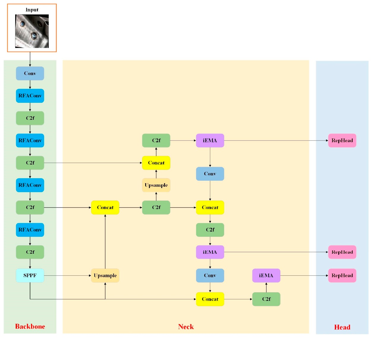
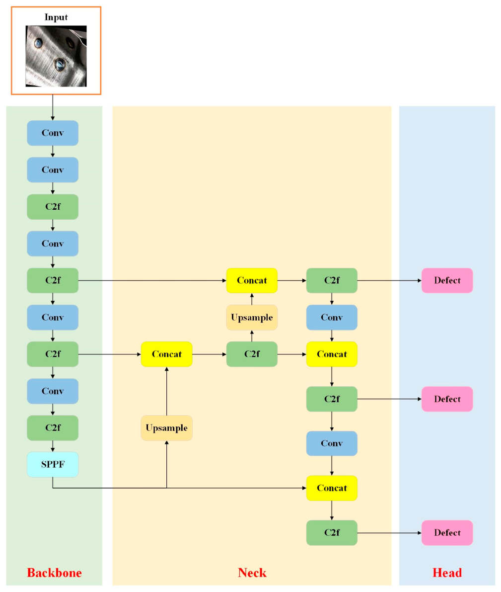
We therefore introduce three modifications to YOLOv8n, with the overall architecture shown in Figure 1 and Figure 2. RFACM is inserted into the backbone to enhance the representation of local weld textures and edge abnormalities through multi-receptive-field feature modelling. The iEMA module combines EMA attention with an inverted residual structure to strengthen information exchange between local details and global context. RepHead is used in the detection head, exploiting multi-branch training and single-branch inference through structural re-parameterization. These modules act on feature extraction, feature enhancement and object prediction, respectively, and jointly improve the stability of weld-defect detection in complex industrial scenes.

2.2. RFACM

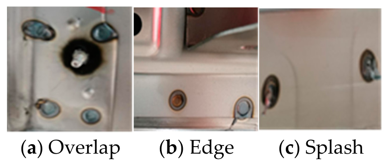
In industrial spot-weld defect detection, the original YOLOv8n backbone mainly extracts features with fixed convolution kernels. This assumes that the same convolution parameters can respond appropriately at different spatial positions. In real weld images, however, defect regions often appear only as local edge damage, splash particles, slight deformations or local texture abnormalities. When defect scales vary markedly and abnormal regions are small, fixed receptive fields can weaken key local information. Figure 3 shows representative samples of edge-defect welds.

Standard convolution (SC) uses fixed kernels and shared parameters, applying the same convolution parameters at different spatial positions. This design is computationally efficient, but it cannot dynamically adjust feature responses to local texture changes in weld regions. Tiny cracks, edge loss, fake welds and slight deformation are often embedded in normal weld structures. Without modelling differences across receptive-field regions, defect information can be overwhelmed by background texture. Standard convolution extracts features with shared kernel parameters, as follows:

$$Y\left(i,j\right)=\sum _m \sum _n W\left(m,n\right)X\left(i+m,j+n\right)$$

(1)

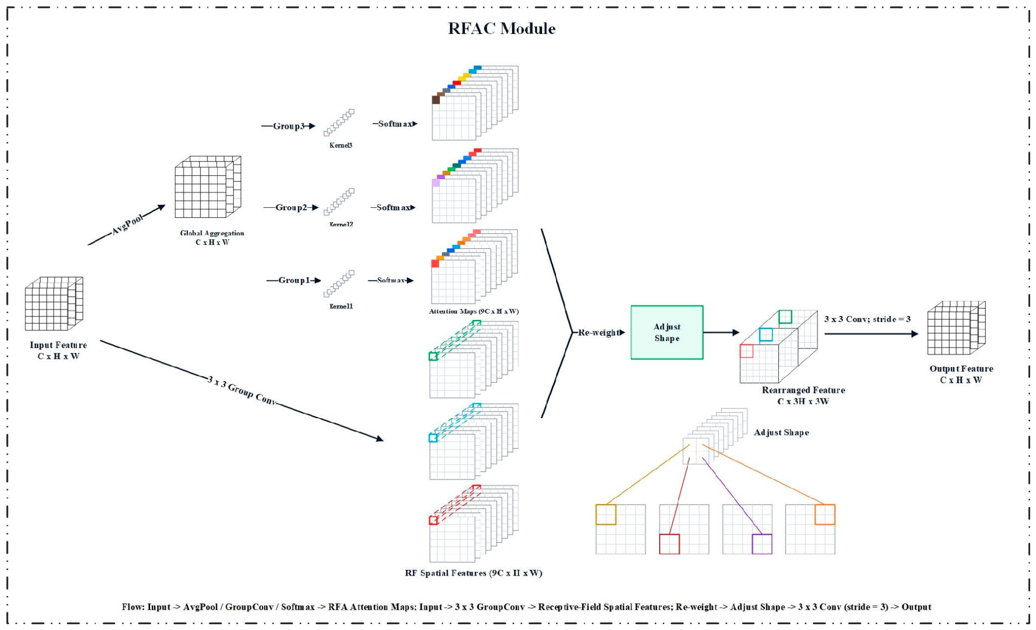
where X denotes the input feature map, W denotes the shared convolution kernel and Y denotes the output feature. Because the convolution parameters are shared across all spatial positions, standard convolution applies the same response to normal and defective weld regions, making it difficult to distinguish edge damage, local splash and background texture. RFACM introduces a receptive-field spatial feature representation [12] by reorganizing local regions within the convolution window. In Figure 4, the upper branch corresponds to global average pooling and grouped 1 × 1 convolution followed by Softmax, which produces the attention maps in Equation (4); the lower branch corresponds to the 3 × 3 grouped convolution that produces the receptive-field features in Equation (2). The re-weighting and shape-adjustment steps implement Equation (5), after which a stride-3 3 × 3 convolution produces the output feature. This explicit mapping links each processing step in Figure 4 with the RFACM equations.

$$F_{rf}=ReLU\left(Norm\left(g_{\left(k\times k\right)\left(X\right)}\right)\right)$$

(2)

where k is the kernel size, and $F_{rf}$ denotes the receptive-field feature map produced by grouped convolution over the local regions. This definition makes Equation (2) explicit and distinguishes $F_{rf}$ from the input feature map X. The grouped convolution operation preserves local spatial structure and texture variation $F_{rf}$.

To further increase attention to key defect regions, RFACM introduces attention-weight learning on the basis of receptive-field features. Global average pooling is first used to obtain global contextual information from the input feature:

$$F_g=AvgPool\left(X\right)$$

(3)

A 1 × 1 grouped convolution is then used to exchange information between different receptive fields:

$$A_{r,f}=Softmax\left({{Conv}_g}^{1\times 1}\left(F_g\right)\right)$$

(4)

The receptive-field attention weights represent the importance of different local regions, and Softmax normalizes the weight distribution. This process adaptively adjusts feature responses according to defect location and texture variation in weld images, encouraging the network to focus on edge abnormalities, local texture changes, morphological damage and abnormal structural regions. Unlike conventional spatial attention, which mainly acts on pixel positions, RFACM applies attention within receptive-field features and therefore produces a weighting scheme better suited to fine-grained weld-defect detection. After receptive-field features and attention weights are obtained, an enhanced feature is generated by element-wise fusion:

$$F=A_{r,f}\times F_{rf}$$

(5)

Through this fusion, RFACM extends fixed convolution into a feature-extraction operation with local adaptive perception, allowing the network to adjust feature responses according to spatial variations in weld-defect regions.

Overall, RFACM is intended to enhance the local representation of small-scale and weak-texture weld defects. For splash, edge loss and fake welds that occupy only local weld regions, RFACM strengthens key textures inside the receptive field. For visually similar classes such as normal welds, fake welds and overlap, dynamic weight allocation improves the discriminability of local features.

2.3. iEMA Module

YOLOv8n extracts features layer by layer through convolutional structures and therefore has high detection efficiency. Nevertheless, convolution primarily models local neighbourhoods. Although the receptive field expands with network depth, semantic associations between distant regions may remain insufficient. In automotive spot-weld inspection, different defect classes can be visually similar. For example, Twist and Overlap both appear as morphological deformation, and Fake regions may resemble background areas. Metallic reflection, weld splash and surface texture further increase the risk of false detection. RFACM strengthens local detail representation, but global context is still needed to support defect discrimination.

Efficient Multi-scale Attention (EMA) can establish long-range dependencies through cross-spatial information interaction with low computational overhead, enabling global context modelling [13]. The original EMA mainly uses attention weights to recalibrate features, but semantic information transfer may still be insufficient in complex industrial scenes. Inverted Residual Mobile Block (iRMB), by contrast, uses an inverted residual structure for efficient feature transfer and helps mitigate information loss in deep networks [14]. We therefore embed EMA attention in a lightweight inverted residual framework to construct iEMA, which combines global context modelling, background-noise suppression and efficient feature transfer.

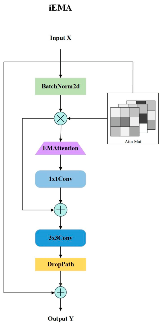
For an input feature map, iEMA first applies Batch Normalization to adjust the feature distribution and improve training stability [15]. The normalized features are then passed into the EMA attention branch. EMA divides the input features into multiple sub-features through grouping and extracts spatial information using convolutions at different scales. The sub-features then enter parallel branches: a 1 × 1 convolution branch builds cross-channel information interaction, while a 3 × 3 convolution branch supplements local spatial texture information. The overall iEMA architecture is illustrated in Figure 5.

$$X=\left[X,, \dots ,X_G\right],X_i \in R^{{\displaystyle \frac{C}{G}}\times H\times W}$$

(6)

$$F_1=\left({Conv}_{1\times 1}\left(X\right)\right)$$

(7)

$$F_2=\left({Conv}_{3\times 3}\left(X\right)\right)$$

(8)

The 1 × 1 convolution branch mainly learns channel dependencies, the 3 × 3 branch supplements local spatial details, and G denotes the number of feature groups. Through multi-scale feature fusion, the network can capture both fine-grained texture information in weld regions and broader contextual information. After multi-scale features are obtained, EMA further uses spatial attention to adaptively adjust the importance of different regions:

$$X_{EMA}=A\odot X$$

(9)

The multi-scale fused features are multiplied element-wise by the spatial attention weights, enhancing defect-region responses while suppressing background noise and irrelevant regions. This operation helps the model recognize weak-texture defects and easily confused classes under complex backgrounds.

To further improve feature-transfer efficiency, a lightweight inverted residual structure from iRMB is introduced after the EMA output. The structure first expands channels through a 1 × 1 convolution, then extracts local spatial features with a depthwise 3 × 3 convolution, and finally restores the channel dimension through another 1 × 1 convolution. Compared with ordinary convolution, depthwise convolution reduces parameters and computation while retaining spatial feature-extraction ability. The enhanced features are then fused with the input features through a residual connection:

$$Y=X+DropPath\left(\left({Conv}_{3\times 3}\left(F\right)\right)\right)$$

(10)

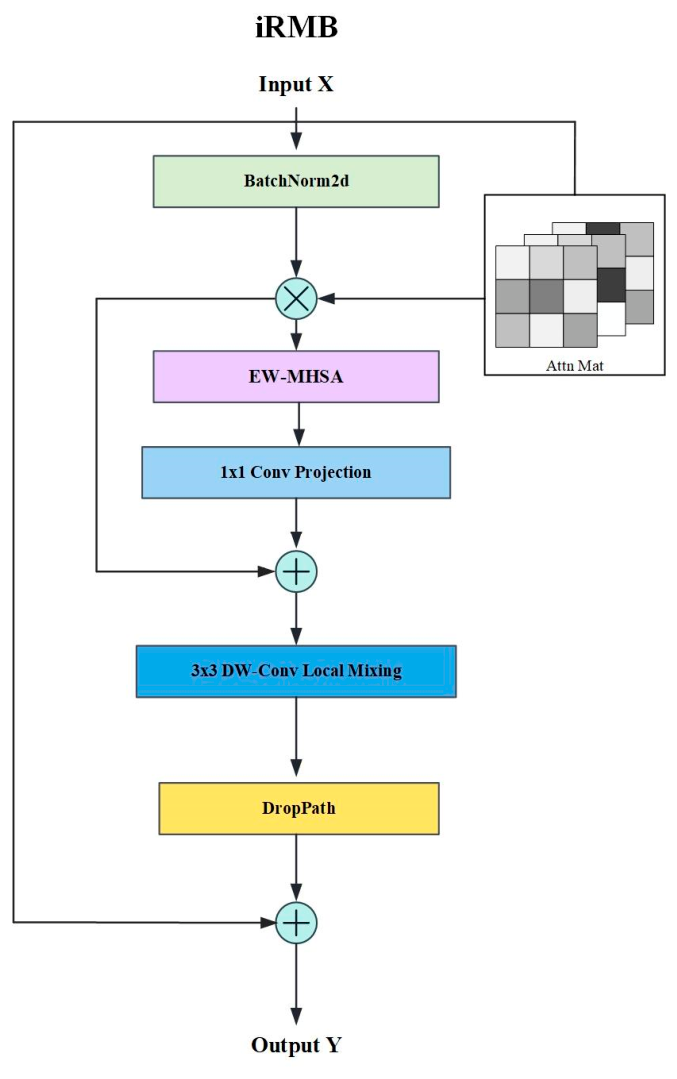
In Equation (10), F denotes the multi-scale feature map after EMA weighting and Y denotes the residual output. DropPath improves generalization during training [16], while the residual connection helps preserve the original feature information. The resulting output is used as the enhanced feature of the iEMA module. The iRMB branch used in this operation is shown in Figure 6.

The iEMA module compensates for the limited global-context modelling of local convolution. EMA attention builds semantic links between the overall weld structure and local defect regions, reducing interference from metallic reflection, welding splash and surface texture. The inverted residual structure improves feature-transfer efficiency, allowing global semantic information to participate more fully in subsequent detection.

2.4. RepHead Module

The original YOLOv8n detection head uses a decoupled structure for bounding-box regression and class prediction, providing high inference efficiency in general object detection. In spot-weld defect detection for automotive structural components, however, splash, fake welds and edge loss are usually small, weak in texture and irregular in boundary shape. The detection head therefore needs stronger feature discrimination between shallow detail features and deep semantic features. Directly stacking more convolution layers or complex multi-branch structures may improve representation during training, but it increases computation and memory-access cost during inference.

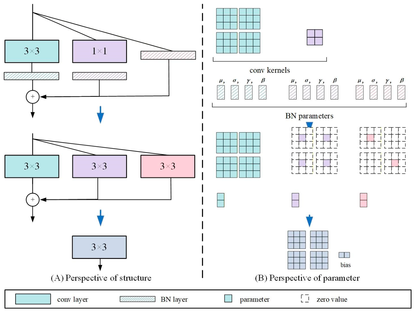
To strengthen detection-head representation while keeping the inference structure compact, we integrate the structural re-parameterization principle from RepVGG [17] into the YOLOv8n detection head and construct RepHead. During training, RepHead uses 3 × 3 convolution, 1 × 1 convolution and identity branches to jointly extract weld-defect features, providing richer gradient paths and stronger local texture modelling. During inference, the multi-branch structure can be equivalently converted into a single 3 × 3 convolutional branch. The overall training and inference structures are illustrated in Figure 7.

Specifically, for an input feature map, the basic re-parameterization unit in RepHead consists of 3 × 3 convolution, 1 × 1 convolution and identity branches during training. When the input and output channel numbers are identical and the stride is 1, the outputs of the three branches are added element-wise:

$$Y=\phi \left({BN}_3\left(W_{3\times 3}\ast X\right)+{BN}_1\left(W_{1\times 1}\ast X\right)+{BN}_0\left(X\right)\right)$$

(11)

where X denotes the input feature map; W3×3 and W1×1 denote the kernels of the 3 × 3 and 1 × 1 convolution branches; BN3, BN1 and BN0 denote the batch-normalization operations in the corresponding branches; phi denotes the nonlinear activation function; and Y denotes the output feature of the RepHead unit during training. When the input and output dimensions differ or the convolution stride is not 1, the identity branch is removed and only the 3 × 3 and 1 × 1 branches are retained.

Because each branch contains convolution and batch normalization, the convolution layer can be fused with the subsequent BN layer before deployment. For any input feature M, the inference process of the BN layer can be written as:

$$BN\left(M_{\mathrm{i}}\right)={\displaystyle \frac{{\gamma }_{\mathrm{i}}\left(M_{\mathrm{i}}-{\mu }_{\mathrm{i}}\right)}{\sqrt{{{\sigma }_{\mathrm{i}}}^2+\epsilon }}}+{\beta }_{\mathrm{i}}$$

(12)

where ${\mu }_{\mathrm{i}}$ and ${\sigma }_{\mathrm{i}}$ squared are the running mean and variance of the i-th output channel, ${\gamma }_{\mathrm{i}}$ and ${\beta }_{\mathrm{i}}$ are the BN scale and bias parameters, and epsilon is a small constant used to prevent division by zero. Equation (12) therefore defines the batch-normalization transform used before branch fusion.

In practice, if the convolution layer has no bias term, $b_{\mathrm{i}}$ can be set to 0. Through this transformation, both the 3 × 3 and 1 × 1 convolution branches can be converted into biased convolution operations. For the 1 × 1 branch, the kernel is expanded into a 3 × 3 kernel by zero padding, with the original 1 × 1 kernel placed at the centre:

$${\tilde{W}}_{1\times 1}=Pad\left({\hat{\mathrm{W}}}_{1\times 1}\right)$$

(13)

The identity branch can likewise be regarded as a special 1 × 1 convolution with an identity-matrix kernel. Let this identity kernel be I. After fusion with BN0, the equivalent kernel and bias of the identity branch are obtained:

$${\hat{\mathrm{W}}}^0={\displaystyle \frac{{\gamma }^{0}I}{\sqrt{{\sigma }^{02}+\epsilon }}}$$

(14)

$${\widehat{b}}^0={\beta }^0-{\displaystyle \frac{{\gamma }^0{\mu }^0}{\sqrt{{\sigma }^{02}+\epsilon }}}$$

(15)

Thus, the multi-branch structure of the RepHead unit during training can be equivalently re-parameterized into a standard 3 × 3 convolution during inference. The final kernel and bias are:

$$Wr={\hat{\mathrm{W}}}_{3\times 3}+Pad\left({\hat{\mathrm{W}}}_{1\times 1}\right)+{\hat{\mathrm{W}}}^0$$

(16)

$$br={\widehat{b}}_{3\times 3}+{\widehat{b}}_{1\times 1}+{\widehat{b}}^0$$

(17)

$$Y=\phi \left(Wr\ast X+br\right)$$

(18)

Through this equivalent conversion, RepHead exploits the multi-branch structure to enhance feature learning during training while retaining only a single-path 3 × 3 convolution during inference. The 3 × 3 branch helps capture local edges, splash particles and burn-through texture changes. The 1 × 1 branch strengthens inter-channel information exchange and improves discrimination between defect classes. The identity branch preserves original feature information and reduces the excessive smoothing of small defects during detection-head mapping. RepHead’s deployment advantage should still be evaluated with actual FPS, per-frame latency and memory use, rather than inferred from GFLOPs or parameter count alone.

In summary, RepHead unifies multi-branch enhancement during training with single-branch re-parameterization during inference. This design can improve detection-head representation for weak-texture, small-scale and irregular-boundary spot-weld defects while maintaining a simplified inference topology.

3. Experimental Results and Analysis

3.1. Experimental Dataset

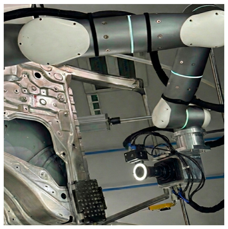
The raw images used in this study were obtained partly from automated enterprise production scenes and partly from a visual acquisition platform built by the research team, as shown in Figure 8. To ensure experimental authenticity, the dataset and sample split were constructed from case data collected during actual welding operations.

The dataset constructed in this study contains 3500 raw images and was divided into training, validation and test sets at a ratio of 8:1:1. LabelImg(version 1.8.6) was used to manually identify and annotate the weld regions of interest in the images, resulting in a total of 13,349 annotated weld instances. The split was performed at the image level. Because component identifiers, collection sequences and production-batch identifiers were not retained, possible correlations between images from the same component or batch cannot be completely excluded and should be examined in a future group-wise split.

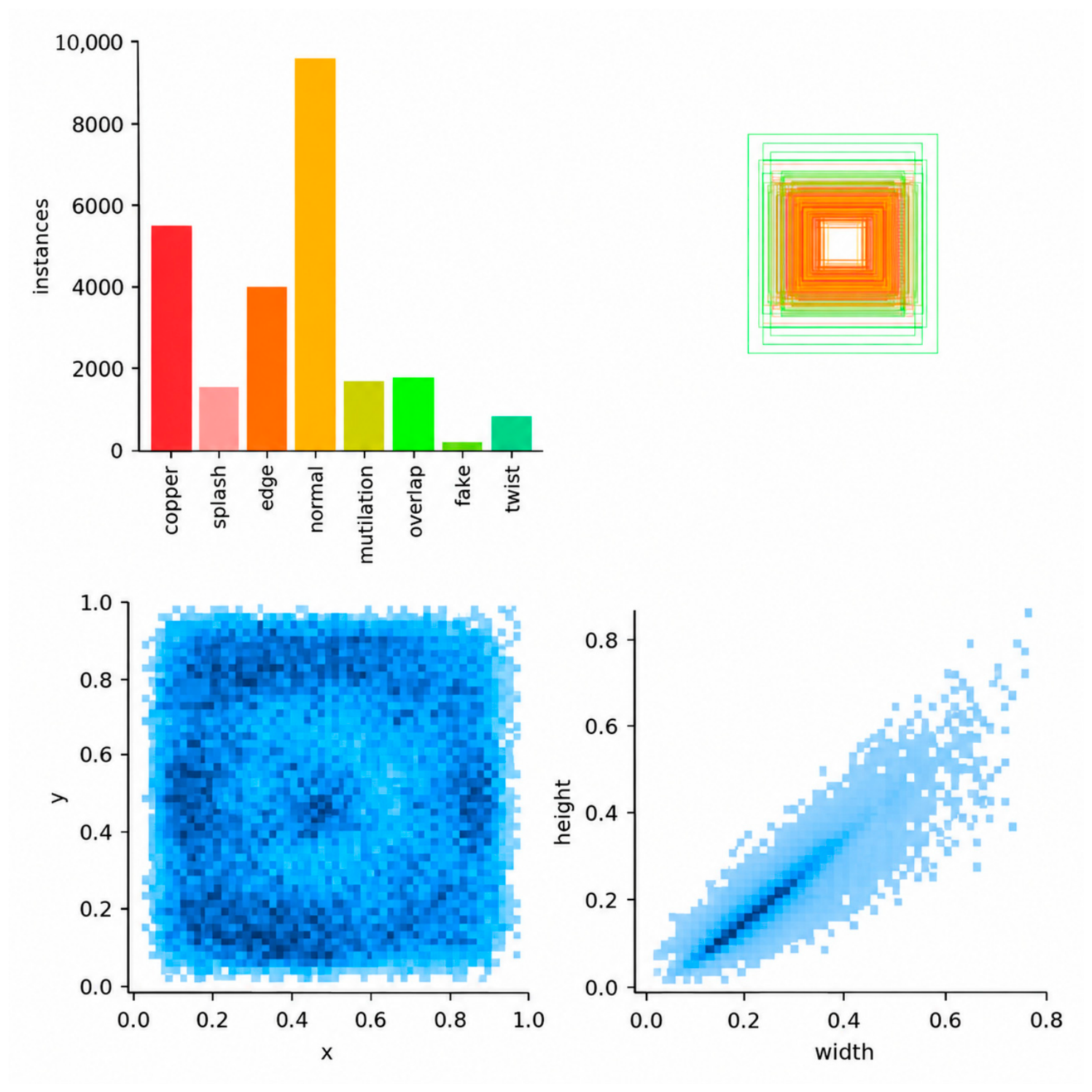
The sample-distribution statistics show that the dataset contains eight weld categories, as shown in Figure 9 and Figure 10. The Normal category contains 10,115 instances, while the remaining seven defect categories contain 3234 instances in total. Therefore, the dataset exhibits a pronounced class imbalance, with Normal samples accounting for approximately 75.77% of all annotated instances. To avoid relying solely on overall detection metrics, the subsequent experiments additionally consider class-wise recognition performance and per-class AP, together with confusion-matrix analysis for the minority defect categories.

3.2. Experimental Settings

To keep model training controllable, development and experiments were conducted on a local laptop, with Jupyter Notebook (version 7.1.2) integrated in Visual Studio Code (version 1.85.2) as the main interactive development environment. Notebook cells were used for model initialization, parameter setting, training monitoring and visualization. The laptop ran 64-bit Windows 11 Professional, with 32 GB physical memory and an NVIDIA GeForce RTX 5070 Laptop GPU with 8 GB video memory. The training platform used the Ultralytics YOLOv8 framework (version 8.3.229), PyTorch (version 2.7.1), CUDA (version13.0) and Python (version3.9.23).

YOLOv8n was used as the base network, initialized with the yolov8n.pt weights. Training used the SGD optimizer with explicit settings for learning-rate scheduling, image augmentation and label smoothing to improve reproducibility. The input image size was 640 × 640, the batch size was 16, and training was run for 100 epochs. The initial learning rate was 0.005 and was dynamically adjusted with cosine annealing. Momentum was set to 0.85 and weight decay to 0.001. To improve robustness, image augmentation included rotation of ±15°, scale ratio of 0.7, colour perturbation (hsv_s = 0.8) and additive noise affecting 1.5% of pixels [18,19]. The label smoothing factor was fixed at 0.4 for the reported run. Because this value is higher than commonly used settings, it should be regarded as a dataset-specific heuristic rather than a generally optimal choice; a dedicated sensitivity analysis remains necessary. Early stopping was enabled and stopped training if validation performance did not improve for 30 consecutive epochs. During validation, the confidence threshold was 0.001, and the IoU threshold for non-maximum suppression was 0.6. To examine sensitivity to stochastic initialization and data-order effects, the training procedure was repeated with independent random seeds while keeping the image split, hyperparameters and evaluation protocol unchanged. For the ablation and NEU-DET experiments, the reported mAP values are expressed as mean ± standard deviation across the completed seed runs. The mean is the point estimate, and the standard deviation describes run-to-run variability.

3.3. Evaluation Metrics

Model performance was evaluated using Precision, Recall, F1, mAP@0.5, mAP@0.5:0.95, parameter count (Params) and computational cost (GFLOPs) [20]. Precision measures the proportion of predicted objects that are correct, Recall measures the proportion of true objects that are detected, and F1 summarizes the balance between Precision and Recall. mAP@0.5 denotes mean average precision at an IoU threshold of 0.5, while mAP@0.5:0.95 evaluates localization quality across multiple IoU thresholds and is more stringent for bounding-box accuracy. Params and GFLOPs measure model complexity, but practical deployment efficiency should also be judged with FPS, per-frame latency and device-side memory use.

$$P={\displaystyle \frac{TP}{TP+FP}}$$

(19)

$$R={\displaystyle \frac{TP}{TP+FN}}$$

(20)

$$mAP={\displaystyle \frac{{\sum }_{i=1}^K {AP}_i}{K}}$$

(21)

$$F_1={\displaystyle \frac{2\times Precision\times Recall}{Precision+Recall}}$$

(22)

TP denotes the number of true-positive samples, FP the number of false-positive samples, FN the number of false-negative samples and TN the number of true-negative samples. Higher Precision indicates fewer false detections, higher Recall indicates fewer missed detections, F1 reflects the combined performance of Precision and Recall, and higher mAP indicates better overall classification and localization performance.

3.4. Ablation Experiments

To verify the effectiveness of the three proposed modules, a series of ablation experiments was designed. The modules include RFACM embedded in the backbone, iEMA for enhanced global-context modelling and the structurally re-parameterized RepHead detection head. By progressively introducing these modules, we compared detection accuracy, parameter count and computational complexity, systematically evaluating each module’s contribution to spot-weld defect detection and the synergy between modules. Visualization results were further used to show the performance of the improved algorithm in complex industrial scenes.

• Ablation experiments

Eight experimental settings were designed around RFACM, iEMA and RepHead. YOLOv8n was used as the baseline. Models with only RFACM, only iEMA and only RepHead were denoted YOLOv8-RFA, YOLOv8-iEMA and YOLOv8-RH, respectively. The model containing all three modules was denoted YOLOv8-RFA-iEMA-RH. All experiments used the same data split and training settings, allowing the contribution of each module to be compared under controlled conditions. The reported ablation and comparison values come from one fixed random seed; no repeated-seed mean or standard deviation was available, so differences of a few tenths of a percentage point should be interpreted descriptively rather than as evidence of statistical significance.

Table 1. Ablation experiments.

Model	Precision (%)	Recall (%)	F1	mAP@0.5 (%)	mAP@0.5:0.95 (%)	Params (M)	GFLOPs (G)
YOLOv8n	89.4	90.4	89.9	95.4 ± 0.12	68.8 ± 0.15	3.4158	8.1
YOLOv8-RFA	89.4	92.0	90.7	96.3 ± 0.16	70.6 ± 0.16	3.0332	8.6
YOLOv8-iEMA	90.0	91.9	90.9	96.4 ± 0.20	71.1 ± 0.16	3.3667	8.8
YOLOv8-RH	89.8	90.9	90.3	95.9 ± 0.10	69.9 ± 0.14	4.0106	8.4
YOLOv8-RFA-iEMA	90.1	91.9	91.0	96.5 ± 0.14	71.3 ± 0.20	3.3731	9.0
YOLOv8-RFA-RH	88.8	92.0	90.4	96.3 ± 0.26	70.5 ± 0.18	4.0409	8.7
YOLOv8-iEMA-RH	89.3	92.3	90.8	96.4 ± 0.18	71.4 ± 0.12	4.2605	9.1
YOLOv8-RFA-iEMA-RH	89.6	92.7	91.2	97.9 ± 0.18	71.9 ± 0.10	4.3869	9.2

shows that each module improved detection performance to varying degrees when introduced individually. RFACM increased mAP@0.5 from 95.4% to 96.3% and mAP@0.5:0.95 to 70.6% while reducing the parameter count to 3.0332 M and GFLOPs to 8.6 G. This suggests that RFACM improves local feature representation while controlling model complexity. iEMA gave strong single-module performance, reaching 96.4% mAP@0.5 and 71.1% mAP@0.5:0.95, indicating that global context modelling supports defect recognition under complex backgrounds. RepHead provided a smaller accuracy gain but reduced GFLOPs to 8.4 G, suggesting that structural re-parameterization may improve the inference structure of the detection head. The standard deviations in the mAP columns are small relative to the corresponding means, indicating that the reported ranking is reasonably stable across the tested seeds. These dispersion estimates describe repeatability within the fixed image split and should not be interpreted as evidence of generalization to unseen production lines.

Pairwise combinations further show complementarity between local multi-receptive-field enhancement and global attention modelling. The RFACM + iEMA combination reached 96.5% mAP@0.5 and 71.3% mAP@0.5:0.95. The iEMA + RepHead combination reached 71.4% mAP@0.5:0.95, indicating that a stronger detection head can further exploit attention-enhanced features. In contrast, the RFACM + RepHead combination reached 70.5% mAP@0.5:0.95, slightly below RFACM alone at 70.6% and clearly below iEMA + RepHead at 71.4%. This negative interaction is consistent with partially redundant local feature enhancement: RFACM changes receptive-field responses in the backbone, whereas RepHead further remaps those features in the head. Without iEMA’s complementary global context, the extra branches may amplify local responses without improving strict localization. The final gain is therefore better explained by the interaction of all three modules, with iEMA providing the main complement to RepHead, rather than by simply stacking modules.

Taken together, RFACM, iEMA and RepHead improved YOLOv8n from three aspects: local texture enhancement, global semantic modelling and detection-head representation. When all three modules are introduced, YOLOv8-RFA-iEMA-RH achieves 97.9% mAP@0.5 and 71.9% mAP@0.5:0.95, improving on the original YOLOv8n by 1.4 and 3.1 percentage points, respectively, within the ablation setting. Because the complete model has a higher parameter count and more GFLOPs than the baseline, it is best described as achieving higher accuracy within a controlled complexity range rather than as a uniformly lightweight model. The Params and GFLOPs reported in Table 1 and

Table 2. Comparison of different models.

Model	Precision (%)	Recall (%)	FPS	mAP@0.5 (%)	mAP@0.5:0.95 (%)	Params (M)	GFLOPs (G)
YOLOv3-tiny	84.9	80.1	34.0	85.4	65.3	12.1307	18.9
YOLOv5	88.3	89.5	45.8	95.2	68.1	2.5041	7.1
YOLOv6	89.4	92.9	19.6	96.7	73.8	16.299	43.7
YOLOv8n	89.4	90.4	41.6	95.3	68.8	3.4158	8.1
YOLOv9t	88.0	91.4	47.5	94.9	69.1	2.0066	7.9
YOLOv10n	88.6	91.3	42.3	96.3	71.4	2.7094	8.4
YOLOv11	90.4	91.3	47.2	96.5	70.9	2.5833	6.3
RT-DETR	89.3	91.2	45.8	96.3	71.1	2.5246	6.9
YOLOv8-RFA-iEMA-RH	89.6	92.7	38.9	97.9	71.9	4.3869	9.2

refer to the graph used for the reported experiments; a separately exported, post-fusion RepHead graph was not benchmarked. The approximately 1M parameter increase in RFACM + RepHead therefore reflects the multi-branch training representation and should not be interpreted as the final deployment overhead.

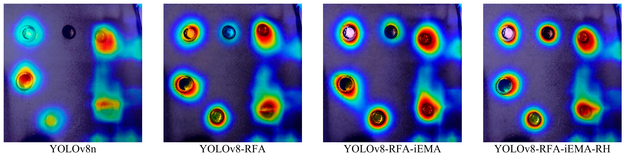
The feature-response heatmaps in Figure 11 provide a qualitative check of the intermediate representations. Relative to YOLOv8n, the progressively enhanced models concentrate stronger responses around weld boundaries and defect-related texture, while suppressing more diffuse background activation. Because these maps are visualization outputs rather than calibrated importance scores, they are interpreted as supporting evidence for the proposed feature-extraction mechanism and not as an independent performance metric.

• Comparative experiments

To further verify the effectiveness of the proposed algorithm, the improved model was compared with mainstream detectors, including YOLOv3-tiny, YOLOv5, YOLOv6, YOLOv8n, YOLOv9t, YOLOv10n, YOLOv11 and RT-DETR. The results are shown in Table 2.

As shown in Table 2, YOLOv8-RFA-iEMA-RH achieved 97.9% mAP@0.5 and a reported throughput of 38.9 FPS. Compared with the YOLOv8n baseline, Recall increased from 90.4% to 92.7%, while FPS decreased from 41.6 to 38.9, a reduction of 2.7 FPS. The model also improved mAP@0.5 from 95.3% to 97.9% and mAP@0.5:0.95 from 68.8% to 71.9%, corresponding to gains of 2.5 and 3.1 percentage points. The FPS values were compared under the same table setting, but the source record did not document warm-up, numerical precision, preprocessing/NMS inclusion or device-side memory. They should therefore be interpreted as reported throughput rather than as complete end-to-end production latency.

Among the other YOLO-family models, YOLOv6 obtained the highest mAP@0.5:0.95 at 73.8%, exceeding the proposed model’s 71.9%. Its parameter count, however, reached 16.30 M, and its GFLOPs reach 43.7 G, which was substantially higher than the proposed model. YOLOv11 had a lower computational cost (6.3 G), but its mAP@0.5 and mAP@0.5:0.95 were 96.5% and 70.9%, both lower than those of the proposed model. RT-DETR is competitive as a Transformer-based detector, but its mAP@0.5:0.95 was 0.8 percentage points lower than that of the proposed model.

The proposed model is therefore not optimal for every single metric. Rather, it provides a favourable compromise among mAP@0.5, Recall and model complexity. Compared with YOLOv6, it remains lower on the stricter localization metric, but it achieves high detection accuracy with fewer parameters and lower computational cost, indicating a better accuracy–complexity balance for the target application.

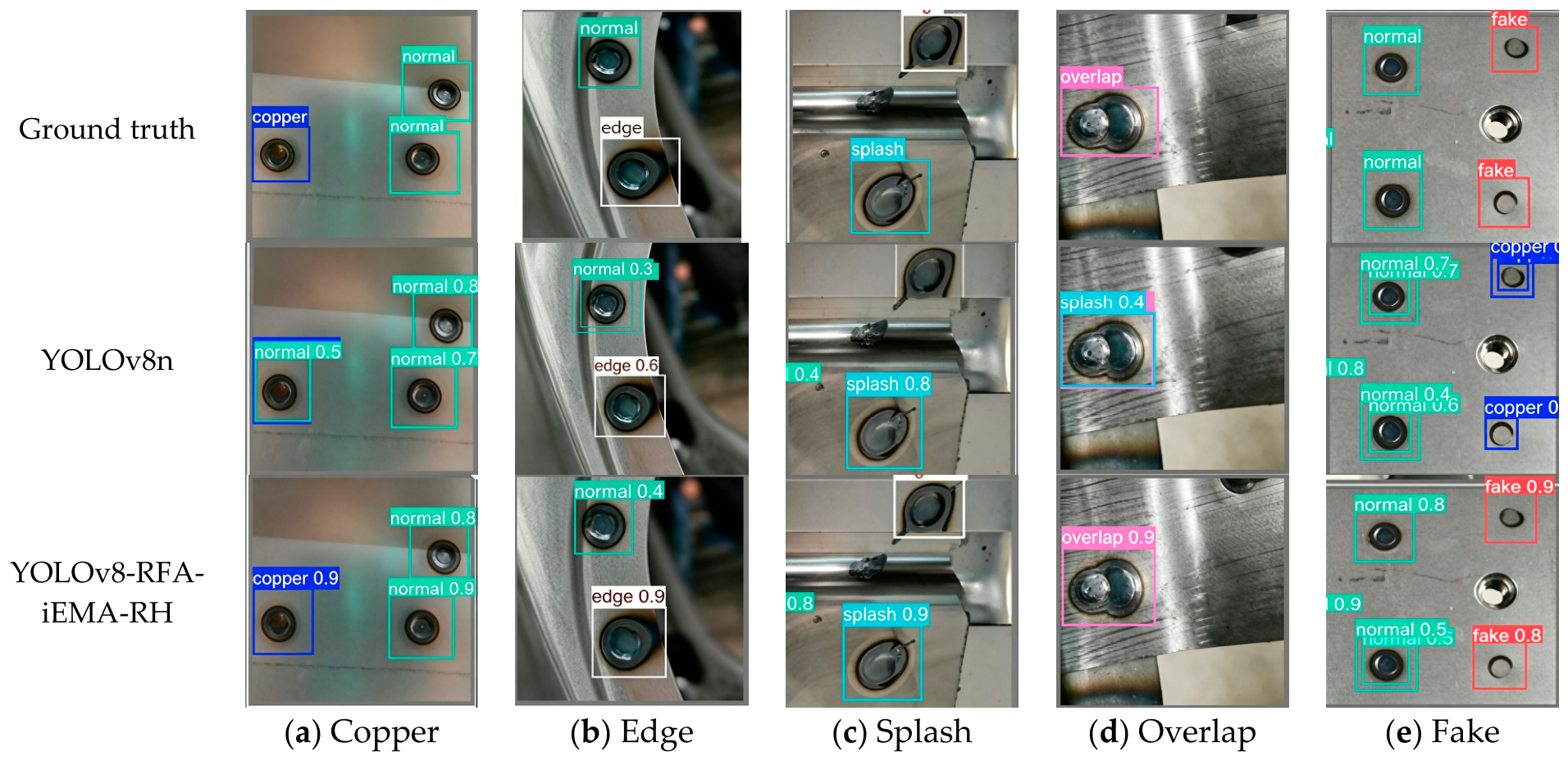
To visually assess YOLOv8-RFA-iEMA-RH relative to YOLOv8n in resistance spot-weld defect detection, ground-truth annotations from the original images were compared with validation-set detection results. The examples cover common defect classes, including Copper, Edge, Splash, Overlap and Fake, as shown in Figure 12.

The detection results are shown in Figure 11. Compared with the original YOLOv8n, the improved model gives more stable detection across several spot-weld defect scenes. For easily confused classes such as Copper and Fake, it reduces some missed detections and misclassifications. For Edge, Splash and Overlap samples with weak edge features or complex backgrounds, its predicted boxes overlap better with the ground truth. This section mainly presents representative successful examples. Future analysis should also include false positives, missed detections and samples where both models fail to more completely define the model’s applicability boundaries.

• Class-wise recognition analysis

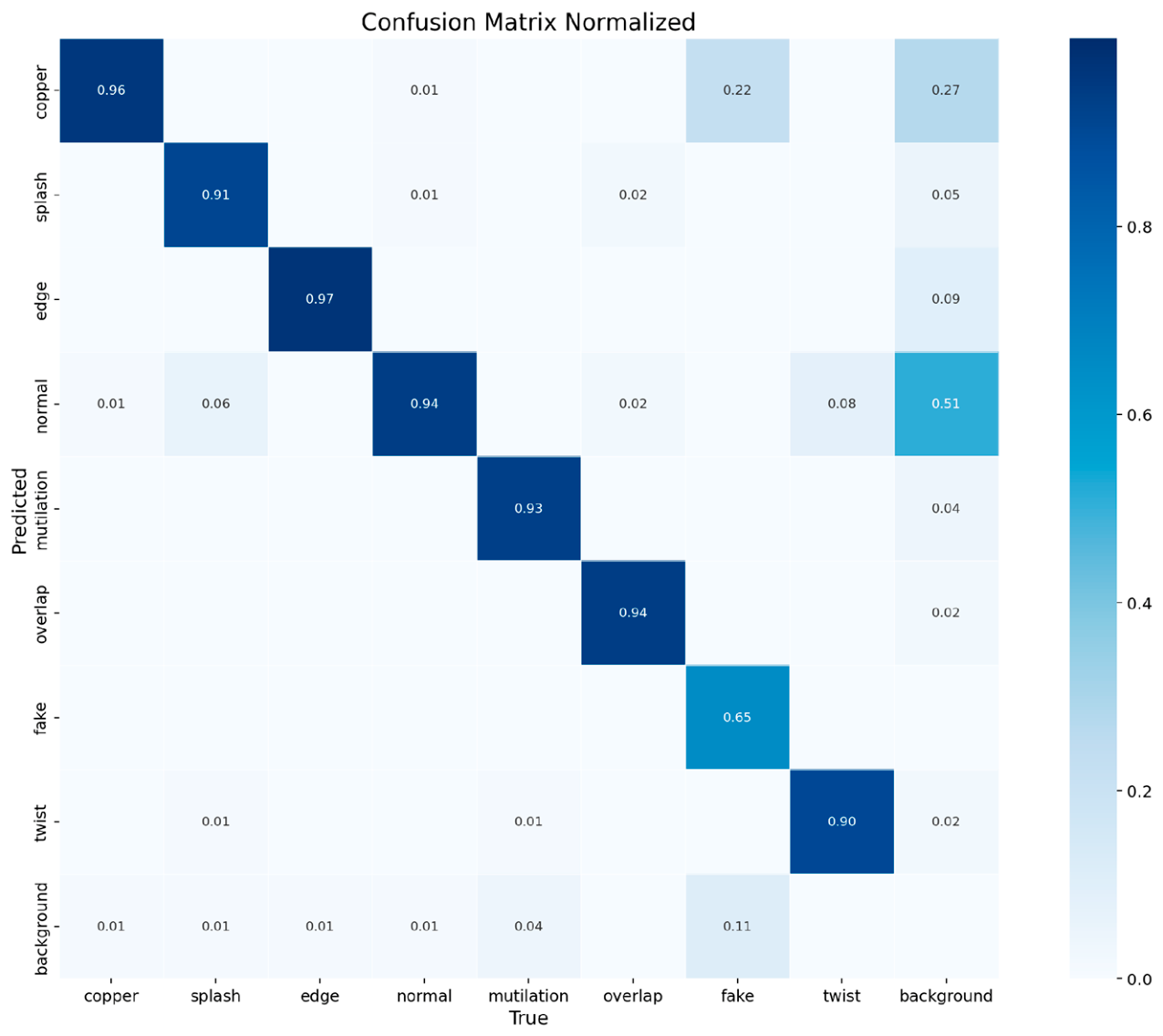
To evaluate the classification and recognition ability of the two models across different spot-weld defect classes, a confusion matrix [20] was used. The horizontal axis represents the ground-truth defect class, and the vertical axis represents the predicted class. Higher values on the diagonal indicate more accurate recognition of the corresponding class, whereas off-diagonal values indicate misclassification or confusion. Comparing confusion-matrix distributions therefore provides an intuitive evaluation of class-wise detection performance.

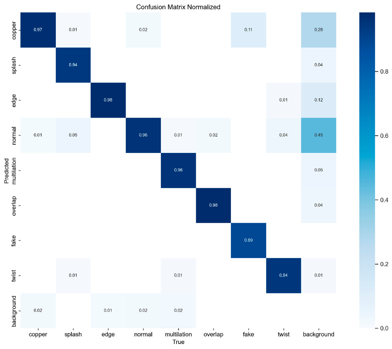
Based on validation-set results, normalized confusion matrices were plotted for YOLOv8n and YOLOv8-RFA-iEMA-RH, as shown in Figure 13 and Figure 14.

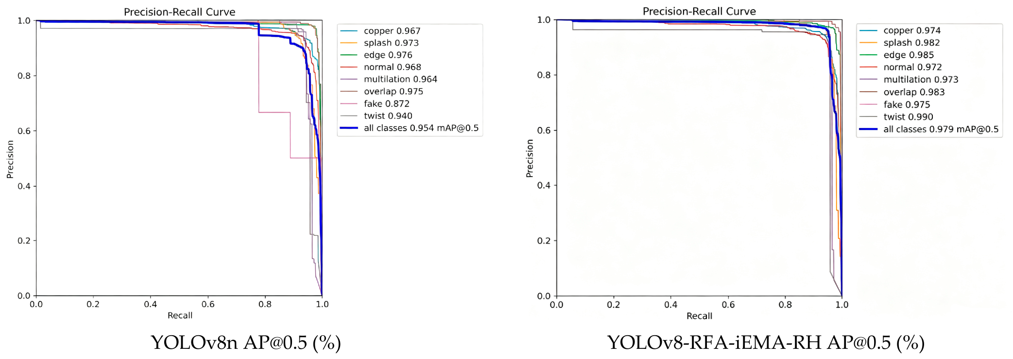
Both models show clear diagonal dominance for the main defect classes, indicating that they learn discriminative features for different spot-weld defects. Compared with the YOLOv8n baseline, the normalized diagonal values of the improved model for Copper, Splash, Edge, Normal, Mutilation, Overlap, Fake and Twist increased from 0.96, 0.91, 0.97, 0.94, 0.93, 0.94, 0.65 and 0.90 to 0.97, 0.94, 0.98, 0.96, 0.96, 0.98, 0.89 and 0.94, respectively. The improvement was most pronounced for Fake, increasing from 0.65 to 0.89, which indicates stronger recognition of weak-texture and easily confused defect classes. Figure 15 reports the corresponding class-wise AP@0.5 values in the order Normal, Copper, Splash, Mutilation, Twist, Overlap, Edge and Fake: 96.8%, 96.7%, 97.3%, 96.4%, 94.0%, 97.5%, 97.6% and 87.2% for YOLOv8n and 98.2%, 97.4%, 98.2%, 97.3%, 95.3%, 99.0%, 98.5% and 97.5% for YOLOv8-RFA-iEMA-RH, respectively. These AP values complement the confusion-matrix results and the aggregate metrics in Table 1 and Table 2. The all-class AP values displayed in the plotted legends should be read as the values associated with the exported precision-recall curves; the tabulated mAP values remain the primary quantitative results because the source record does not document whether the curves and tables used identical evaluation exports.

The off-diagonal distribution shows that the baseline model is unstable for the Fake class, with some samples misclassified as Copper or Background. The improved model markedly strengthened the diagonal response for Fake and reduced confusion with visually similar weld classes. Consistent with this pattern, Fake AP@0.5 increased from 87.2% to 97.5% in Figure 15. The AP curves show that the largest gain occurred for the minority Fake class, whereas the already strong classes changed more modestly. These results suggest that RFACM-enhanced local receptive-field textures, iEMA-based global context modelling and RepHead-based detection-head representation act complementarily to improve class discrimination under complex backgrounds. Background regions are still sometimes misclassified as Normal, Copper or Edge, indicating that background areas and weld regions retain similar local texture and reflection patterns.

• Cross-dataset validation

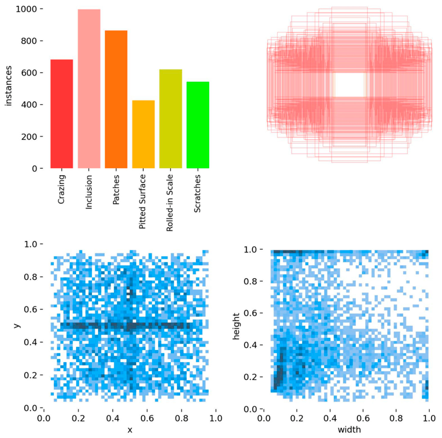
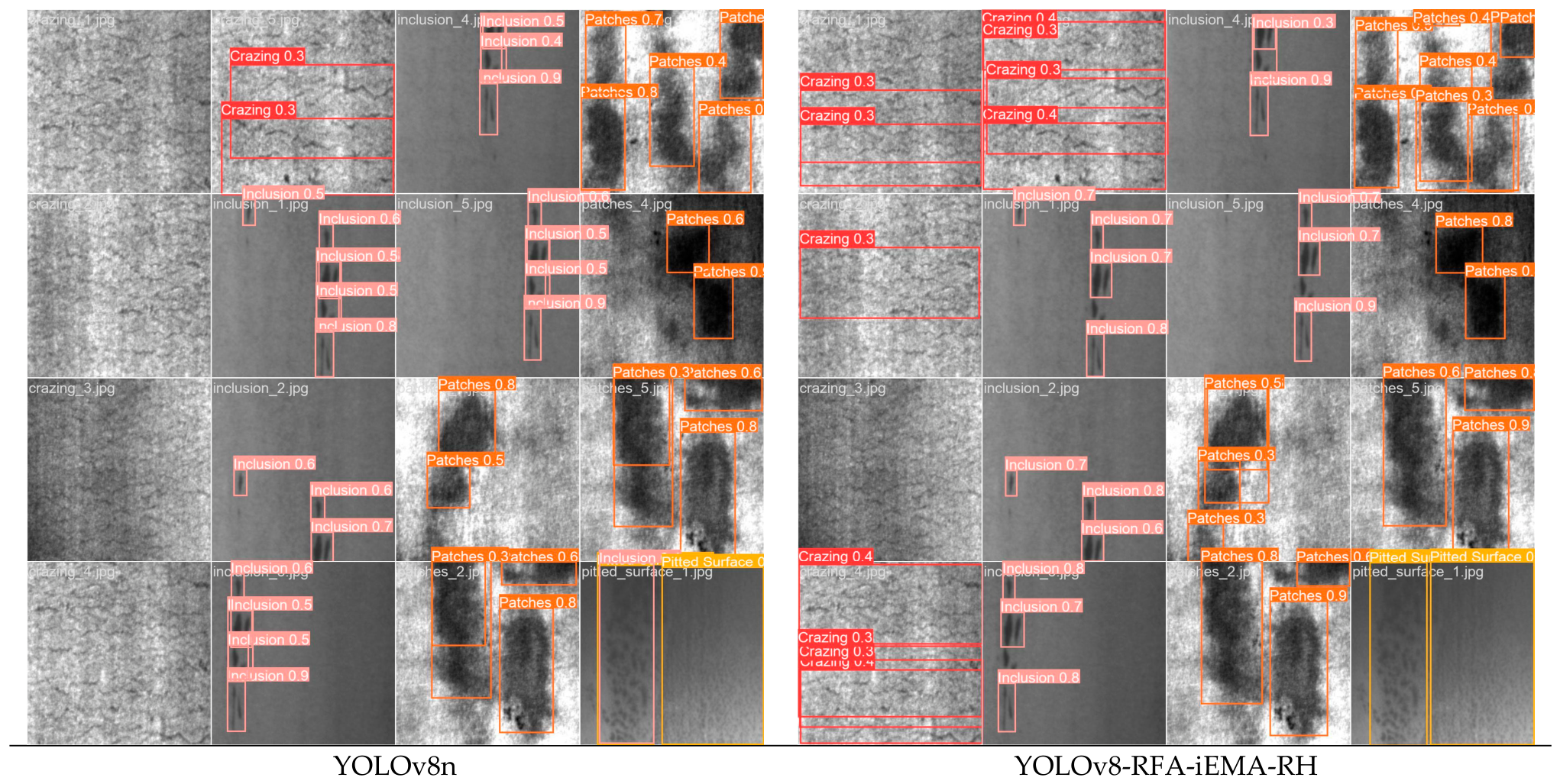
To preliminarily evaluate adaptability to other industrial surface-defect scenes, the NEU-DET steel surface defect dataset provided by Northeastern University was used for cross-dataset validation [21]. Comparisons of different defect types are shown in Figure 16, Figure 17 and Figure 18. The dataset contains 1799 images from six defect types: crazing, inclusion, patches, pitted surface, rolled-in scale and scratches. For this auxiliary experiment, YOLOv8n and YOLOv8-RFA-iEMA-RH were each trained on the NEU-DET training split and evaluated on the held-out validation split using the same 640 × 640 input size, batch size 16, SGD optimizer and fixed seed. Because NEU-DET differs from automotive spot-weld images in object morphology and imaging conditions, it is used here as a domain-shifted auxiliary test rather than as direct evidence of generalization to real spot-weld production lines. The experimental protocol and data split are reported together with the quantitative comparison in

Table 3. Comparison of two models for steel defect detection.

Model	Precision (%)	Recall (%)	F1	mAP@0.5 (%)	mAP@0.5:0.95 (%)	Params (M)	GFLOPs (G)
YOLOv8n	64.6	68.3	66.4	71.1	43.3	3.068	8.1
YOLOv8-RFA-iEMA-RH	79.5	69.8	74.3	78.8	48.7	4.387	9.2

.

The results are shown in Table 3. Compared with the original YOLOv8n, the proposed model improved performance on NEU-DET to different extents. Precision increased from 64.6% to 79.5%, a gain of 14.9 percentage points; Recall increased from 68.3% to 69.8%, a gain of 1.5 percentage points; F1 increased from 66.4% to 74.3%, a gain of 7.9 percentage points; mAP@0.5 increased from 71.1% to 78.8%, a gain of 7.7 percentage points; and mAP@0.5:0.95 increased from 43.3% to 48.7%, a gain of 5.4 percentage points. Although the parameter count increased from 3.068 M to 4.387 M and GFLOPs from 8.1 G to 9.2 G, the computational complexity remained moderate. These results indicate that the proposed method has some adaptability to steel surface defect detection. Because NEU-DET differs from the automotive spot-weld task, however, the results should be interpreted only as cross-dataset validation, and model stability still needs further testing on multi-scene spot-weld data and in real production environments.

4. Conclusions and Outlook

This study proposed an improved YOLOv8n-based algorithm for spot-weld defect detection in automotive structural components, addressing large target-scale variation, complex background interference and limited detection accuracy. The algorithm integrates RFACM into the backbone to enhance local texture representation, constructs iEMA to strengthen global context modelling, and uses a structurally re-parameterized RepHead to improve detection-head feature learning while retaining a simplified inference topology. On the self-built spot-weld defect dataset, the improved model achieved 92.7% Recall, 91.2% F1, 97.9% mAP@0.5 and 71.9% mAP@0.5:0.95, improving on the original YOLOv8n across these metrics in the reported split. Ablation and comparative experiments verify the descriptive contribution of the proposed modifications, while the RFACM+RepHead result shows that RepHead was not uniformly beneficial without complementary global-context modelling. Experiments on the public NEU-DET dataset further showed a degree of domain-shifted adaptability, but they should be interpreted as auxiliary cross-dataset evaluation rather than direct evidence of generalization to automotive production scenes. Several limitations remain: the class imbalance requires further class-wise error analysis on an independently grouped split; although repeated-seed results and standard deviations are now reported for the ablation and NEU-DET experiments, confidence intervals and formal significance tests were not prespecified; and actual device-level inference speed, end-to-end latency and memory consumption were not fully benchmarked after RepHead fusion. Future work will focus on group-wise multi-scene spot-weld data, prespecified statistical analysis, detailed per-class evaluation and deployment-oriented benchmarking on representative industrial hardware.

References

1. Feng, Y.; Wang, Y.; Liu, F. Four-diagnosis and four-dimensional analysis method for open weld problems in automotive body spot welding. Automob. Maint. 2025, 5–10. [Google Scholar]
2. Yang, C.; Wang, Y.; Hu, Y.; Wang, W. Vehicle minor damage detection algorithm based on deep learning. Comput. Eng. Des. 2025, 46, 2986–2993. [Google Scholar]
3. Jocher, G.; Chaurasia, A.; Qiu, J.; Jaiswal, A.; Mehta, A.; Karthik, R.; Mankowski, D.; Qiao, S.; Ultralytics Team. Ultralytics YOLOv8. 2023. Available online: https://github.com/ultralytics/ultralytics (accessed on 7 September 2026).
4. Lin, T.Y.; Dollár, P.; Girshick, R.; He, K.; Hariharan, B.; Belongie, S. Feature Pyramid Networks for Object Detection. In Proceedings of the IEEE Conference on Computer Vision and Pattern Recognition; IEEE: Honolulu, HI, USA, 2017; pp. 2117–2125. [Google Scholar]
5. Liu, S.; Qi, L.; Qin, H.; Shi, J.; Jia, J. Path Aggregation Network for Instance Segmentation. In Proceedings of the IEEE Conference on Computer Vision and Pattern Recognition; IEEE: Salt Lake City, UT, USA, 2018; pp. 8759–8768. [Google Scholar]
6. Hu, J.; Shen, L.; Sun, G. Squeeze-and-Excitation Networks. In Proceedings of the IEEE Conference on Computer Vision and Pattern Recognition; IEEE: Salt Lake City, UT, USA, 2018; pp. 7132–7141. [Google Scholar]
7. Woo, S.; Park, J.; Lee, J.Y.; Kweon, I.S. CBAM: Convolutional Block Attention Module. In Proceedings of the European Conference on Computer Vision; Springer: Munich, Germany, 2018; pp. 3–19. [Google Scholar]
8. Hou, Q.; Zhou, D.; Feng, J. Coordinate Attention for Efficient Mobile Network Design. In Proceedings of the IEEE/CVF Conference on Computer Vision and Pattern Recognition; IEEE: Nashville, TN, USA, 2021; pp. 13713–13722. [Google Scholar]
9. Lu, M.; Sheng, W.; Zou, Y.; Chen, Z. WSS-YOLO: An Improved Industrial Defect Detection Network for Steel Surface Defects. Measurement 2024, 245, 115060. [Google Scholar] [CrossRef] [Scilit]
10. Zhang, T.; Pan, P.; Zhang, J.; Zhang, X. Steel Surface Defect Detection Algorithm Based on Improved YOLOv8n. Appl. Sci. 2024, 14, 5325. [Google Scholar] [CrossRef] [Scilit]
11. Luo, Y.; Ling, J.; Wang, J.; Zhang, H.; Chen, F.; Xiao, X.; Lu, N. SFW-YOLO: A Lightweight Multi-Scale Dynamic Attention Network for Weld Defect Detection in Steel Bridge Inspection. Measurement 2025, 257, 117608. [Google Scholar] [CrossRef] [Scilit]
12. Zhang, X.; Liu, C.; Yang, D.; Song, T.; Ye, Y.; Li, K.; Song, Y. RFAConv: Innovating Spatial Attention and Standard Convolutional Operation. arXiv 2023, arXiv:2304.03198. [Google Scholar] [CrossRef] [Scilit]
13. Ouyang, D.; He, S.; Zhang, G.; Luo, M.; Guo, H.; Zhan, J.; Huang, Z. Efficient Multi-Scale Attention Module with Cross-Spatial Learning. arXiv 2023, arXiv:2305.13563. [Google Scholar] [CrossRef] [Scilit]
14. Zhang, J.; Li, X.; Li, J.; Liu, L.; Xue, Z.; Zhang, B.; Jiang, Z.; Huang, T.; Wang, Y.; Wang, C. Rethinking Mobile Block for Efficient Attention-based Models. arXiv 2023, arXiv:2301.01146. [Google Scholar] [CrossRef] [Scilit]
15. Ioffe, S.; Szegedy, C. Batch Normalization: Accelerating Deep Network Training by Reducing Internal Covariate Shift. In Proceedings of the 32nd International Conference on Machine Learning; PMLR: Lille, France, 2015; pp. 448–456. [Google Scholar]
16. Huang, G.; Sun, Y.; Liu, Z.; Sedra, D.; Weinberger, K.Q. Deep Networks with Stochastic Depth. In Proceedings of the European Conference on Computer Vision; Springer: Amsterdam, Netherlands, 2016; pp. 646–661. [Google Scholar]
17. Ding, X.; Zhang, X.; Ma, N.; Han, J.; Ding, G.; Sun, J. RepVGG: Making VGG-style ConvNets Great Again. In Proceedings of the IEEE/CVF Conference on Computer Vision and Pattern Recognition, Nashville, TN, USA, 19–25 June 2021; pp. 13733–13742. [Google Scholar] [CrossRef] [Scilit]
18. Krizhevsky, A.; Sutskever, I.; Hinton, G.E. ImageNet Classification with Deep Convolutional Neural Networks. Adv. Neural Inf. Process. Syst. 2012, 25, 1097–1105. [Google Scholar]
19. Shorten, C.; Khoshgoftaar, T.M. A survey on Image Data Augmentation for Deep Learning. J. Big Data 2019, 6, 60. [Google Scholar] [CrossRef] [Scilit]
20. Tharwat, A. Classification assessment methods. Appl. Comput. Inform. 2021, 17, 168–192. [Google Scholar] [CrossRef] [Scilit]
21. Song, K.; Yan, Y. A noise robust method based on completed local binary patterns for hot-rolled steel strip surface defects. Appl. Surf. Sci. 2013, 285, 858–864. [Google Scholar] [CrossRef] [Scilit]
Figure 1. YOLOv8 network architecture.
Ai 07 00379 g001
Figure 2. YOLOv8-RFA-iEMA-RH network architecture.
Ai 07 00379 g002
Figure 3. Weld images with edge defects.
Ai 07 00379 g003
Figure 4. RFACM architecture and equation mapping. Different colors denote different receptive-field groups and their corresponding spatial positions within the convolution window. Solid colored squares indicate the selected receptive-field elements, whereas dashed lines and arrows represent grouping, reshaping, or feature-routing operations. The upper branch generates receptive-field attention maps using global average pooling, grouped 1 × 1 convolution and Softmax (Equation (4)). The lower branch constructs receptive-field spatial features through grouped 3 × 3 convolution (Equation (2)). The re-weighting and shape-adjustment operations correspond to Equation (5), followed by a 3 × 3 convolution with stride 3 to produce the output feature.
Ai 07 00379 g004
Figure 5. Overall architecture of iEMA. Overall architecture of iEMA. Solid blocks denote feature tensors and convolutional transformations; dashed arrows denote residual or reshape routing; the 1 × 1 and 3 × 3 branches represent channel-interaction and local-spatial processing, respectively. The diagram follows Equations (6)–(10): grouping, multi-scale convolution, attention weighting, projection, local mixing, DropPath and residual addition.
Ai 07 00379 g005
Figure 6. iRMB architecture. Solid blocks denote pointwise expansion, depthwise spatial mixing and pointwise projection; the dashed shortcut denotes residual addition. The block follows the inverted-residual design used after EMA weighting.
Ai 07 00379 g006
Figure 7. RepHead structural re-parameterization. During training, the 3 × 3, 1 × 1 and identity branches are optimized jointly; before inference, convolution–BN fusion, kernel padding and branch summation merge them into one equivalent 3 × 3 branch. Coloured solid blocks indicate the three trainable branches, and the dashed arrow indicates the deployment-time fusion path.
Ai 07 00379 g007
Figure 8. Visual platform for image acquisition.
Ai 07 00379 g008
Figure 9. Sample distribution of spot-weld defects. Counts of five or more digits use comma separators.
Ai 07 00379 g009
Figure 10. Eight spot-weld morphologies.
Ai 07 00379 g010
Figure 11. Feature-response heatmap comparison of ablation models.
Ai 07 00379 g011
Figure 12. Visual comparison of detection results. Overlapping boxes are retained where they correspond to distinct ground-truth instances; no overlap obscures the class labels or prevents scientific interpretation.
Ai 07 00379 g012
Figure 13. YOLOv8n confusion matrix.
Ai 07 00379 g013
Figure 14. YOLOv8-RFA-iEMA-RH confusion matrix.
Ai 07 00379 g014
Figure 15. Class-wise precision-recall curves and class-wise AP@0.5.
Ai 07 00379 g015
Figure 16. Sample distribution of steel surface defects.
Ai 07 00379 g016
Figure 17. Examples of steel surface defects.
Ai 07 00379 g017
Figure 18. Experimental comparison of the two models. The panels are arranged to avoid overlap; the figure position may be adjusted during production.
Ai 07 00379 g018