Semi-Supervised Generative Adversarial Networks (GANs) for Adhesion Condition Identification in Intelligent and Autonomous Railway Systems

Abstract

Safe and reliable railway operation forms an integral part of autonomous transport systems and depends on accurate knowledge of the adhesion conditions. Both the underestimation and overestimation of adhesion can compromise real-time decision-making in traction and braking control, leading to accidents or excessive wear at the wheel–rail interface. Although limited research has explored the estimation of adhesion forces using data-driven algorithms, most existing approaches lack self-reliance and fail to adequately capture low adhesion levels, which are critical to identify. Moreover, obtaining labelled experimental data remains a significant challenge in adopting data-driven solutions for domain-specific problems. This study implements self-reliant deep learning (DL) models as perception modules for intelligent railway systems, enabling low adhesion identification by training on raw time sequences. In the second phase, to address the challenge of label acquisition, a semi-supervised generative adversarial network (SGAN) is developed. Compared to the supervised algorithms, the SGAN achieved superior performance, with 98.38% accuracy, 98.42% precision, and 98.28% F1-score in identifying seven different adhesion conditions. In contrast, the MLP and 1D-CNN models achieved accuracy of 91% and 93.88%, respectively. These findings demonstrate the potential of SGAN-based data-driven perception for enhancing autonomy, adaptability, and fault diagnosis in intelligent rail and robotic mobility systems. The proposed approach offers an efficient and scalable solution for real-time railway condition monitoring and fault identification, eliminating the overhead associated with manual data labelling.

1. Introduction

Among the various parameters of railway systems, the adhesion force is one of the most critical and complex parameters which plays an essential role in designing the traction and braking systems of the railway vehicle. Maintaining the adhesion level between the track and wheel is essential for safe operation and it depends on various operational and environmental parameters [1]. The adhesion level of the wheel–rail interface depends upon multiple parameters, many of which are difficult to measure or cannot be determined. Thus, it is required to go through various steps for adhesion condition estimation using these factors. It is reported that complex inter-relations between the dynamics of the wheel–rail interface are required during estimating adhesion force [2].

Adhesion affecting factors are generally classified as operational and environmental. Operational factors which are generally taken into account are kinematic oscillations of the conical wheelset, geometric parameters of the wheel and rail, disturbances in lateral or longitudinal direction, rotational dynamics, vehicle weight distribution on the contact patch, velocity of the vehicle and vehicle design [3,4,5]. Similarly, the environmental factors include weather conditions, temperature, natural contaminations such as dirt, snow, water and synthetic third body materials applied on the rail head [6].

Among various railway dynamics, the adhesion force is considered as a very complex phenomenon and it is also difficult to investigate it while considering all the parameters which directly impact on it [7,8]. Thus, there is not any single synergetic approach available that can determine it while considering all the related factors. The majority of the research work reported in this area covers few parameters and assumes ideal conditions for other parameters [9]. The research work done in this domain reports that there is no direct method to measure adhesion level [7,10]. However, it can be estimated from other relevant parameters of the wheel–rail interface. Various methods have been investigated for the adhesion estimation [7] including model-based such as Kalman filter and its different variants, estimation theory-based methods and inverse modelling techniques which are widely used for adhesion estimation. Currently, deep learning (DL) has surfaced as a potential approach for the condition monitoring of the railway assets and has been applied in various applications and its outstanding performance is reported in other domains [11,12].

Therefore, this paper presents a generative adversarial network (GAN)-based adhesion level identification mechanism to explore the potential of advanced data-driven approaches within autonomous and intelligent railway systems. To enable the effective identification of adhesion levels, we propose a semi-supervised data-driven model, referred to as SGAN, that contributes to real-time perception and control tasks. Accurate adhesion level identification is essential for the proper characterisation of traction and braking forces in autonomous transport and robotic mobility contexts. Furthermore, to extend the capabilities of deep learning (DL) architectures, a self-reliant adhesion identification framework is also investigated, capable of efficiently detecting various adhesion conditions, including those derived from unlabelled data.

The core contributions, positioned within the scope of autonomous system design and robotic perception, can be summarised as follows:

• A GAN-based semi-supervised model is developed to enhance the performance of data-driven methods for fault detection and perception-driven decision-making under low adhesion conditions.
• Simulations were conducted using a validated wheelset dynamic model to generate adhesion condition data for evaluating the proposed semi-supervised learning framework.
• A comparative analysis with conventional supervised data-driven algorithms was carried out to validate the efficacy of the proposed GAN-based perception model.
• The results demonstrate that the proposed approach is suitable for real-time railway adhesion condition monitoring and autonomous traction–braking control, offering a self-sufficient, data-driven DL framework that supports autonomous decision-making without dependence on labelled data.

The remainder of this paper is organised as follows: Section 2 reports the literature, Section 3 discusses the methods, Section 4 describes the data-driven techniques, and Section 5 reports and discusses the results. We conclude this paper in Section 6.

2. Related Works

The methods used for estimating the adhesion force can be categorised into two main streams including model-based and data-driven approaches. These streams are discussed below.

2.1. Model-Based Approaches

The major hurdle for constructing a mathematical manifestation of a physical system is the identification and incorporation of all the necessary variables that have an impact on the model behaviour. Model-based approaches have been employed to a great extent for adhesion identification [13]. The adhesion force is a highly complex phenomenon and for its estimation all the related factors cannot be taken into consideration at the same time. Therefore, researchers have implemented various models of wheelset, bogie, and full vehicle for different research purposes [14].

A single wheelset model has to be the optimal choice for the analysis of the adhesion conditions [7]. Hence, the model is extensively used for that purpose. K. Mal et al. in [15] have presented a mathematical model of a wheel for investigating the adhesion coefficient produced at the wheel–rail contact which was aimed to determine the relation between the adhesion coefficient, slip ratio and yaw rate. Furthermore, nature-inspired computation-based methods such as the Particle Swarm Optimisation (PSO) algorithm have also been investigated by some researchers [16]. However, the methods do not yield the convergence of the optimisation algorithm. Kalman filter has been extensively used for adhesion estimation purposes. In this direction, K. Mal et al. in [17] have employed a wheelset model and investigated the traction and braking modes of vehicles to determine the calculation and estimation of change in adhesion conditions during the operation of the vehicle. They have considered conditions. EKF is designed to estimate dry, wet, greasy and extremely contaminated wheel–rail contact conditions and then is implemented on two different FPGA systems for its functional verification. The authors of [18] have estimated the wheel–rail contact conditions and added a fuzzy logic block in the model-based estimator for its validation. Similarly, the authors in [16] used the wheelset dynamic model proposed by Garg et al. [14] to determine the creep forces. The obtained forces were further investigated using the unscented Kalman filter (UKF) to determine the contact condition. Furthermore, a joint UKF is employed to estimate friction at the contact patch without reusing the residuals obtained.

In [19], the authors have explored the variations in wheelset speed to determine the contact force for better controlling the slip. The authors have extended this work in [20], where slip velocity is estimated using an extended Kalman filter (EKF). The EKF is inputted with measured wheel speed which is tuned with multiple configurations. The authors of [21] have employed a wheelset model to investigate the slip/slide of the wheel and re-adhesion control of traction motors in locomotives. The proposed method employs EKF which was provided with inputs from traction motors including current, voltage and speed. This work was further extended by the authors of [22] where an UKF is investigated to estimate roller friction. Goodall et al. [23] have developed a bogie model which only considers the lateral dynamics of the body. The research covers the four adhesion conditions. An EKF-based method is employed for the identification of low adhesion and to achieve an indirect mechanism for determining the vehicle dynamic response.

In [24], the authors have developed a two-dimensional (2D) and full railway vehicle model. The research has tried to fully explore the complicated model to its advantage. This research is further explored by E. Meli et al. [25]. The 2D model has been upgraded to a three-dimensional (3D) model. The position and orientation of the 3D model were calculated along with its lateral and longitudinal motion. Strano et al. [26] have employed EKF for contact force estimation. The research was performed using a full vehicle model considering yaw and lateral dynamics. The research involved two different adhesion conditions which were labelled as high and low adhesion through quantitative analysis. In [8], the authors have presented an onboard-vehicle monitoring system to estimate the friction coefficient and creep by using the curve fitting approach. In [27], another variant of the Kalman filter, Kalman–Bucy filter (KBF), is combined with the least square technique to determine the adhesion level.

As observed from the aforementioned studies, the Kalman filter [28] and its variants such as EKF, UKF, and KBF have been widely employed for the estimation of adhesion, contact force, friction and other parameters in the railway domain [29], whereas novel mathematical observer-based methods are also implemented for that purpose.

Table 1. Summary of the model-based approaches.

Research	Model Type	Estimation Method	Modelled Parameters	Estimated Parameters
[8]	Single wheelset	Curve fitting	N/A	Friction coefficient and creep
[14]	Do	Model	N/A	N/A
[15]	Do	EKF	Lateral track disturbance and traction torque	Adhesion coefficient, slip ratio and yaw rate
[16]	Do	UKF	Do	Adhesion coefficient, slip ratio and yaw rate in switching of adhesion conditions
[17]	Do	EKF	Do	Do
[19]	Do	EKF	Track disturbances and velocity	Adhesion, slip velocity, and forces
[21]	Do	EKF	Do	Do
[22]	Half vehicle	UKF	Yaw and lateral dynamics	Adhesion coefficient
[23]	Complete bogie	EKF	Track disturbances and velocity	Adhesion, slip velocity, and forces
[24]	Complete vehicle	Model	Angular velocity/acceleration	Adhesion coefficient and forces
[25]	Do	Model	Do	Do
[26]	Do	EKF	Yaw and lateral dynamics	Adhesion coefficient
[27]	Do	KBF with least square technique	N/A	Creep forces
[29]	Locomotive/ measured data	EKF	Track disturbances, velocity	Adhesion, slip velocity, and forces

summarises the reviewed model-based approaches in this section.

2.2. Data-Driven Approaches

The data-driven approaches known as machine learning or deep learning (ML/DL) have been widely employed in various domains such as healthcare, robotics, business, and industry. These approaches have outperformed the traditional methods. Machine learning and deep learning algorithms are used [30,31,32] for the anomaly detection of railway wheel flats and railway tracks. However, these methods have been employed very limitedly for the identification of the adhesion force between wheel–rail interfaces. In this direction, the authors of [33] have used a single wheel model to acquire simulation data consisting of velocity difference and acceleration. These data are further used to develop a supervised Neural Network (NN) model with backpropagation to classify different adhesion levels. S.Falomi et al. in [34] have explored an NN-based approach to detect wheel–rail contact points. M.Malvezzi et al. [35] employed a hybrid method for estimating the adhesion condition. They collected the experimental data of three different parameters including longitudinal velocity, rotational velocity, and the brake cylinder pressure under artificially yielded low adhesion conditions. Li et al. [36] have developed an adhesion control mechanism based on a hybrid model-based on genetic algorithms (GAs) and NNs. J.J.Castillo et al. in [37] have presented a KF- and fuzzy logic (FL)-based EH brake system, whereas an NN is employed to estimate the optimal slip. However, the study did not consider adhesion estimation as a major part of the investigation.

Apart from the aforementioned research, some researchers have used a variety of ML algorithms for the identification of the adhesion level at the wheel–rail contact. In [38], a multi-condition rail surface state image dataset is constructed and a “GoogLeNet as the teacher and MobileNet as the student” co-optimisation framework is established. The proposed multi-source fusion strategy integrates rail surface condition information with maximum adhesion coefficient estimation. In [39] the authors have used an auto-encoder (AE) and support vector machine (SVM) models to classify the adhesion for a road vehicle. They obtained the data through a sliding mode cascading (SMC) observer which was implemented to measure the slip velocity and adhesion coefficient from load torque. The authors of [40] used an AE model in an unsupervised configuration. They considered a single dry creep curve in the research and identified various operating points. In [41], the authors have generated real data from a hardware in loop (HIL) simulation to train a kernel extreme learning machine (KLEM) model. However, it relied on the same observer which does not appear as self-sufficient owing to its dependence on the feature generation or estimation approaches. S. Sreshta et al. [7] have comprehensively reviewed the adhesion estimation methods and provided conclusions that these methods have not yet yielded effective results for adhesion estimation. In our published research [42], we employed a multiple supervised machine learning method for adhesion identification from raw input with a focus on low adhesion conditions. The wheelset dynamic model and Polach-based simulation framework used for data generation are consistent with those reported in our earlier study [42] and are reused here as a validated physical baseline for evaluating the proposed learning framework. In this paper, improved results based on semi-supervised GAN are presented.

Table 2. Summary of the data-driven methods used in railway research area.

Research	Supervised	Self-Sufficient	Low Adhesion Estimation
[33]	Yes	No	Yes
[34]	Yes	Only explores the contact points identification
[35]	Yes	No	Not tested
[36]	Adhesion identification is not carried out
[37]	Adhesion identification is not carried out
[39]	Yes	No	No
[40]	Unsupervised	No	No
[41]	Yes	No	No
[42]	Yes	Yes	Yes
Proposed Method	Semi-supervised	Yes	Yes

summarises the work conducted in the railway domain through data-driven methods.

Compared to the existing research, this paper presents a novel semi-supervised method for adhesion condition identification through generative adversarial methods. Efforts are put in to investigate the potential of DL architectures to develop a self-reliant adhesion identification method which can effectively classify the low adhesion levels from unprocessed data.

3. Proposed Experimental Design

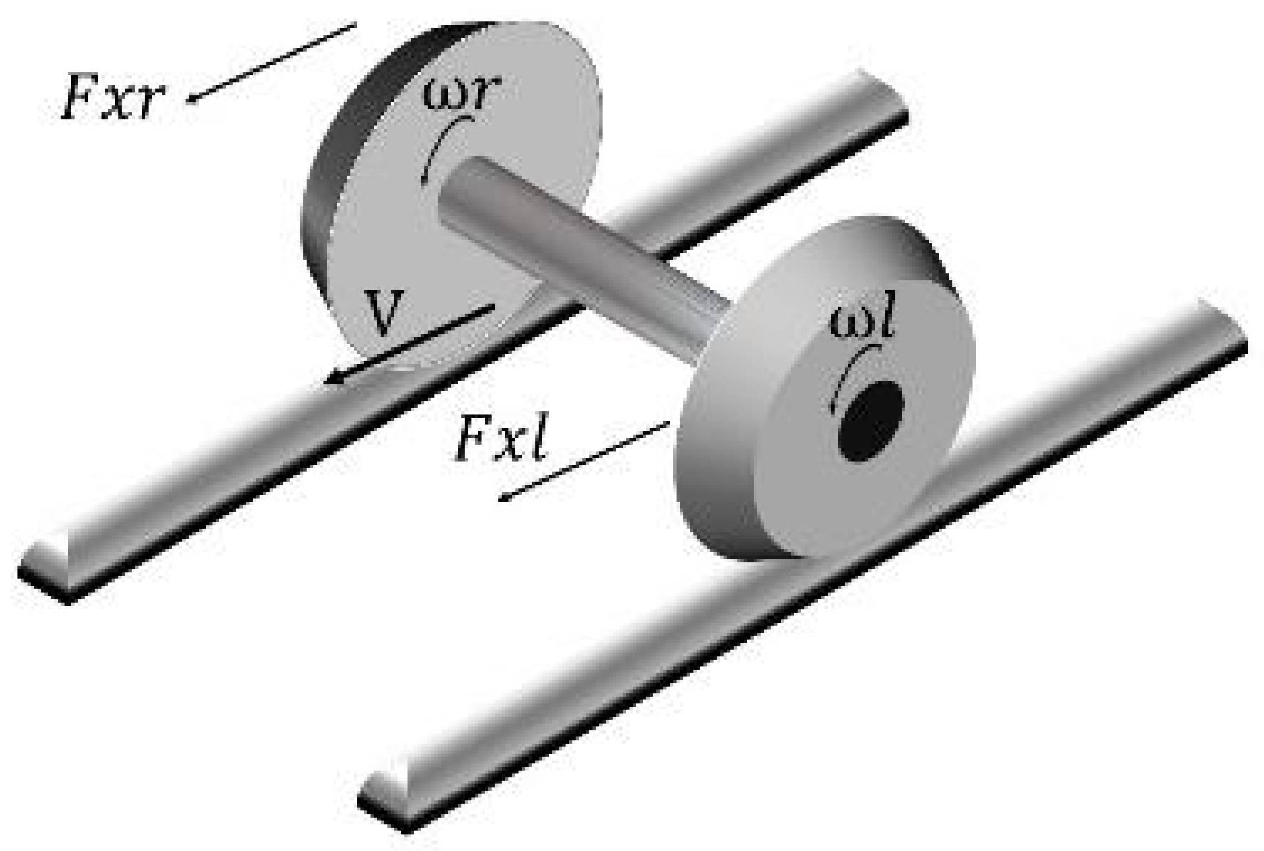
A solid axle wheelset model (shown in Figure 1) with lateral and yaw dynamics is considered as the optimal approach to carry out the adhesion classification analysis [7,23]. An indirect mechanism can be established for online adhesion information extraction from the model by exploiting the variations in the rotational and lateral dynamics in the presence of track disturbances [10,22,27]. Thus, a wheelset model with lateral and yaw dynamics is selected to carry out the investigation for implementing the adhesion identification method proposed in this research. The model and adhesion identification techniques are discussed in the following subsections.

3.1. Wheelset Modelling

Developing a mathematical manifestation of the creep is of paramount importance as it defines the dynamics of the wheel–rail contact. The wheel rolling over the steel track moves rarely in a pure roll motion due to the elastic deformation. Slip/skid of the wheel is a common occurrence that needs to be formulated as well. The creep of a solid axle wheelset could be analysed by observing the variation in the respective angular velocities of both wheels [2]. The distribution of the normal load onto narrow contact also need to be accounted for. During initial contact, both bodies in contact are compressed and adhesion takes place for a short instant. Subsequently, decompression occurs when the bodies are exiting the contact patch, leaving the track part in tension [43].

The adhesion coefficient relates the normal load to the traction effort and the relation can be expressed by Equation (1).

$$\mu ={\displaystyle \frac{F}{W.g}}={\displaystyle \frac{Tractioneffort}{Normalload}}$$

(1)

where F represents traction force, w represents weight, and g is the acceleration due to gravity.

Mathematically, creep is observed via analysing the relative motion of the vehicle with respect to the track. Creep could be observed in both the longitudinal and lateral directions. The longitudinal creep γx can be expressed by Equation (2) [2].

$${\gamma }_x={\displaystyle \frac{V_w-V_v}{V_v}}$$

(2)

where V_v represents the forward speed of the vehicle body and is calculated using Equation (3) and V_w represents the effective speed under the impact of creep.

$$V_v={\omega }_v.r$$

(3)

where ω_v denotes the angular velocity of the wheel and r denotes the contact radius which continuously varies owing to the lateral disturbances caused by the track and the conical shape of wheels. The lateral disturbances make certain that the forward velocities of individual wheels vary proportionally with the variations in the disturbances rather than maintaining the same velocities. For that case, the forward speed of the vehicle can be expressed as in Equations (4) and (5) for the left and right wheels, respectively. For simplification of expressing the relations, the wheelset has been considered as moved in the right direction.

$$V_{wL}={\omega }_{wL}.[r_o+{\lambda }_w(y_w-y_t)]$$

(4)

$$V_{wR}={\omega }_{wR}.[r_o-{\lambda }_w(y_w-y_t)]$$

(5)

where ω_wL, ω_wR denote the angular velocities of both wheels, whereas r_o represents the initial value of the contact radius when the wheel is aligned and centred. Similarly, λ_w denotes the conicity of the wheelset. The wheel profile is assumed to be a pure conical shape and standard wheel profiles are not taken into consideration [9]. Track disturbances in the lateral direction when the vehicle is in motion are denoted by y_t. Lateral disturbances having a random nature have been introduced in the model whose amplitude has been limited according to the minimum and maximum values which the wheel can tolerate without derailing. Generally, many other parameters such as track gauge, wheelset alignment, cross level, and wheelset profile could be taken into consideration but since this work studies the yaw and lateral motion of the model, only track disturbances are induced [2]. Meanwhile, the yaw motion of the wheelset also plays an important role in longitudinal creep in the reverse directions of individual wheelsets [44]. The longitudinal creepage for the left wheel and right wheel are expressed by Equations (6) and (7) respectively:

$${\gamma }_{xL}={\displaystyle \frac{r_o{\omega }_{wL}-V_v}{V_v}}+[{\displaystyle \frac{L_g{\psi }_w}{V_v}}+{\displaystyle \frac{{\omega }_{wL}{\lambda }_w(y_w-y_t)}{V_v}}]$$

(6)

$${\gamma }_{xR}={\displaystyle \frac{r_o{\omega }_{wR}-V_v}{V_v}}+[{\displaystyle \frac{L_g{\psi }_w}{V_v}}+{\displaystyle \frac{{\omega }_{wR}{\lambda }_w(y_w-y_t)}{V_v}}]$$

(7)

where L_g and ψ_w denote the half gauge of the track and yaw angle of the wheels, respectively. The y_w represents the lateral displacement of the wheel. Lateral creep could also be present due to lateral disturbances and the wheel running at an angle of attack to the track. Lateral creep represented by γ_y [2] is given in Equation (8).

$${\gamma }_y={\gamma }_{yR}={\gamma }_{yL}={\displaystyle \frac{\stackrel{.}{{\displaystyle y_w}}}{V_v}}-{\psi }_w$$

(8)

Spin creep also significantly effects the lateral creep but the wheelset modelled in this research is considered a pure conical shape without any flange [1]. Thus, the total creep magnitude in both the directions can be expressed as

$${\gamma }_R=\sqrt{{{\gamma }_{xR}}^2+{{\gamma }_y}^2}$$

(9)

$${\gamma }_L=\sqrt{{{\gamma }_{xL}}^2+{{\gamma }_y}^2}$$

(10)

Creep forces are generated when the vehicle moves along the track under the effect of creep [2,45]. This phenomenon has been exclusively analysed by Kalkar who presented a mathematical model defining the contact forces [46]. Kakar’s contact theory laid the basis of all the further research work reported on tangential force generation and its effects.

Creep forces cause a damping effect when creep is very low and are considered very helpful for stabilisation in those specific regions of operation. In this condition, adhesion is effective over the full contact area owing to the theory of normal contact by Hertz. According to the theory, the creep and creep force are linearly related to each other, and the relation is given by (11) and (12) [47]:

$$F_{xj}=f_{11}{\gamma }_{xj}, j=L,R$$

(11)

$$F_y=f_{22}{\gamma }_y$$

(12)

where f₁₁ and f₂₂ represent adhesion force coefficients and the slope of the creep curve at the region of operation of the wheelset. The contact forces become non-linear with the raise in creep and at the point where the damping effect by the forces is insignificant. This region of operation demonstrates a highly non-linear behaviour with the slope of the quickly varying creep curve. The contact forces of the left and right wheels in both the directions are given by (13) and (14):

$$F_{iR}=F_R.{\displaystyle \frac{{\gamma }_{iR}}{{\gamma }_R}}$$

(13)

$$F_{iL}=F_L.{\displaystyle \frac{{\gamma }_{iL}}{{\gamma }_L}}$$

(14)

where F_xR, F_xL, F_yR, and F_yL represent the contact forces of both the right and left wheels in both directions, respectively. The F_R and F_L represent contact force magnitudes for both the wheels at the narrow contact area which vary with respect to the vertical load and adhesion.

$$F_j={\mu }_j{N}_j, j=L,R$$

(15)

The equation takes the adhesion coefficient as the input and is obtained from Polach’s model [48]. Meanwhile, the above equations are primarily important for this investigation and were the target for explaining the railway vehicle dynamics’ thorough fundamental properties. Since this investigation is aimed at the directly measurable quantities including longitudinal linear velocity, angular velocities of both the wheels, and twist angle of the vehicle, these quantities are directly measurable using appropriate sensors. These quantities can be found using the following equations:

$$V=({\displaystyle \frac{1}{M_v}}.{\displaystyle \int (F_{xR}+F_{xL})dt})+V_o$$

(16)

where M_v represents the mass of the vehicle, F_xR is the creep force of the right wheel in the longitudinal direction, F_xL is the creep force of the left wheel in the longitudinal direction, and v0 represents the initial forward velocity of the vehicle.

$${\omega }_R=({\displaystyle \frac{1}{I_R}}.{\displaystyle \int (T_m-T_s-T_R)dt})+{\omega }_o$$

(17)

where T_m is the torque of the traction motor, T_s represents torsional torque, T_R traction torque on the right wheel, ɷ_R represents the angular velocity of the right wheel, and ɷ_o represents the initial angular velocity of the wheelset.

$${\omega }_L=({\displaystyle \frac{1}{I_L}}.{\displaystyle \int (T_s-T_L)dt})+{\omega }_o$$

(18)

where T_L is the traction torque on the left wheel and ɷ_L represents the angular velocity of the left wheel.

$${\theta }_s={\displaystyle \int ({\omega }_R-{\omega }_L)dt}$$

(19)

where θ_s represents the twist angle.

3.2. Simulating Adhesion Conditions

Polach’s model is used for generating different adhesion conditions [48]. The following equations are employed in the simulation of different adhesion conditions using the model.

$$F={\displaystyle \frac{2Q\mu }{\pi }}({\displaystyle \frac{\epsilon }{{\epsilon }^2+1}}+\arctan \epsilon )$$

(20)

$$\mu ={\mu }_o[(1-A)e^{(-BVc)}+A]$$

(21)

$$\epsilon ={\displaystyle \frac{2}{3}}{\displaystyle \frac{c\pi a^{2}b}{Q\mu }}S$$

(22)

In (20) F denotes the adhesion force, µ denotes the friction coefficient, Q denotes wheel load, and ε represents the gradient of tangential stress in the area of adhesion which is calculated using (22). In (21), A and B denote the curve tuning factors, and V_c represents creep velocity. From (22), a, b are half axes of the contact ellipses, C is contact sheer stiffness, and the total creep is represented by s.

The curve tuning factors A and B in the Polach model were selected to represent the progressive degradation of wheel–rail adhesion. Specifically, A varies from 0.4 under dry conditions to 0.1 under extremely low adhesion, while B varies from 0.6 to 0.2 across the same range, with intermediate values assigned for wet, medium, low, very low, and very very low adhesion conditions. These values follow the standard Polach-based modelling practice reported in the literature and were adopted to emulate realistic creep–adhesion behaviour. The wheel load was assumed constant throughout the simulations to isolate the effect of adhesion variation on the dynamic response.

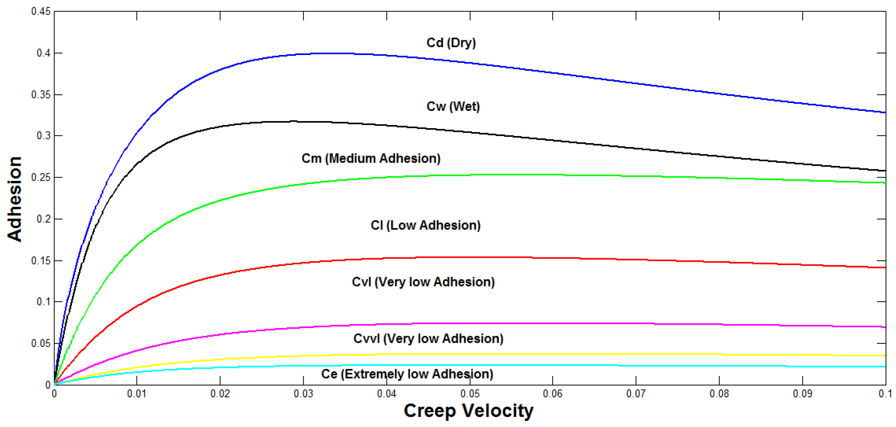
In this study, the simulation framework is primarily designed to investigate reduced adhesion regimes within the saturated region of the creep–adhesion characteristic. Accordingly, seven adhesion conditions are considered and labelled as C1–C7, representing progressively decreasing wheel–rail adhesion levels. These include dry (C1), wet (C2), medium adhesion (C3), low adhesion (C4), very low adhesion (C5), very very low adhesion (C6), and extremely low adhesion (C7). These labels are used consistently throughout Figure 2, Figure 3, Figure 4, Figure 5 and Figure 6 to indicate the adhesion condition under which the wheelset responses are generated.

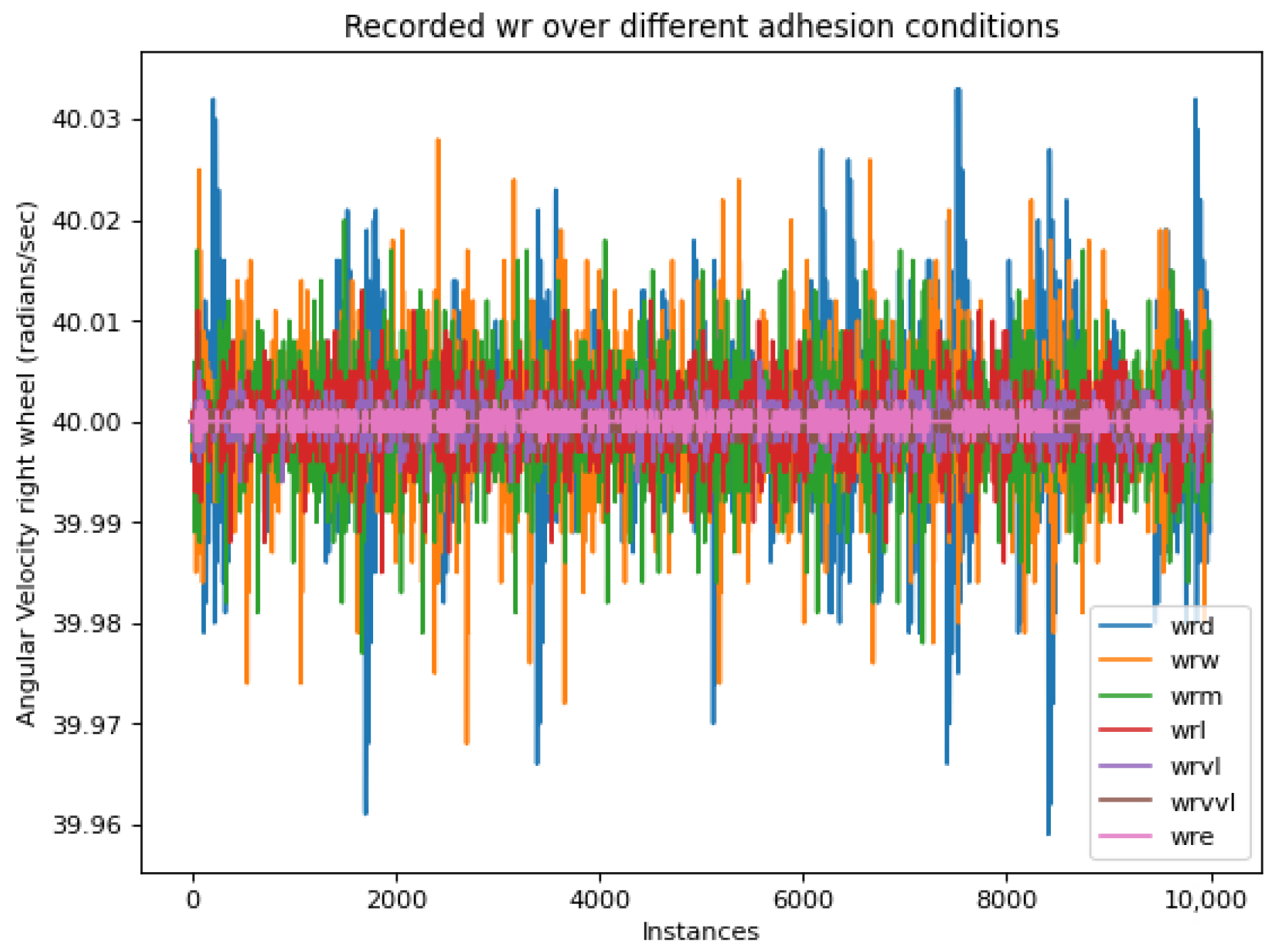
The directly measurable quantities including angular velocities of the wheels, longitudinal velocity, and twist angles are measured and investigated. The Figure 2, Figure 3, Figure 4 and Figure 5 depict the responses obtained from the wheelset model. It should be noticed that the x-axis of the following plots is given as instances rather than seconds because this investigation does not focus on time and the spectral properties of these signals. The data obtained in this research are a sequential type of data and the first ten thousand samples obtained from the model are plotted in the following figures.

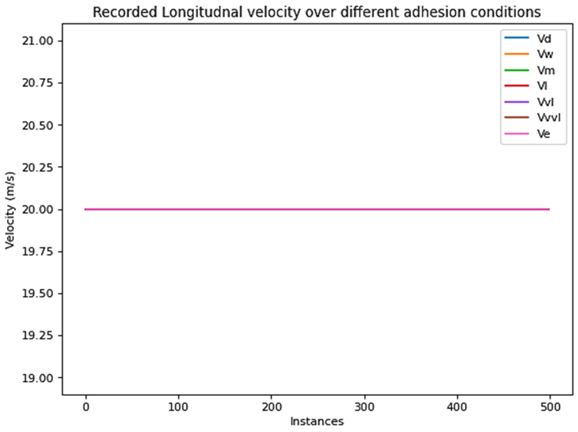
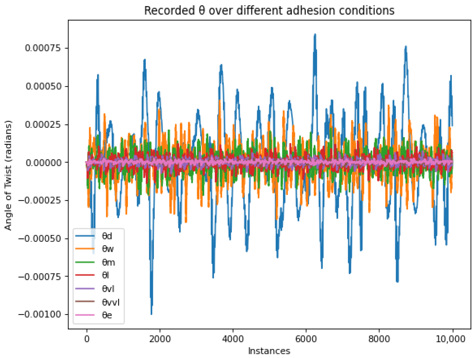
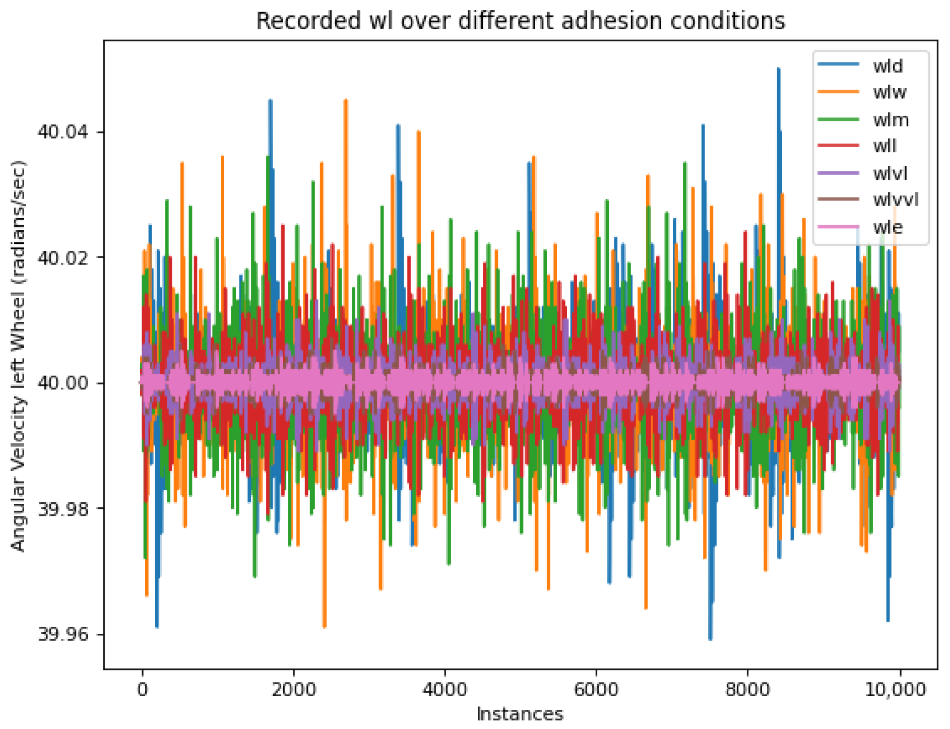
As depicted in Figure 2, variations in lateral disturbances and adhesion levels to the wheelset model have no significant impact on the longitudinal velocity. Thus, velocities at different adhesion levels are overlapped with one another. Figure 4 and Figure 5 depict the angular velocities of both the wheels at different adhesion levels. From the figures, it can be noticed that the frequency of the angular velocities increases and the amplitude decreases under different adhesion conditions. Figure 3 also shows the similar response in which the twist angle is plotted against the seven adhesion levels.

In addition to implementing a self-reliant data-driven solution for the adhesion estimation, this investigation is particularly focused on the low adhesion levels. Thus, the seven different adhesion levels are simulated in this research by employing Polach’s model. The adhesion levels were modelled for the saturated lower adhesion region. Hence, among the seven adhesion levels, four levels fall in the lower adhesion region. The adhesion levels include dry (C1), wet (C2), medium adhesion (C3), low adhesion (C4), very low adhesion (C5), very very low adhesion (C6), and extremely low adhesion (C7), which are depicted in Figure 6, where C1, C2, C3, C4, C5, C6, and C7 are the labels assigned to the adhesion levels.

3.3. Data Collection and Preparation

Polach’s model is used for the manifestation of the contact conditions; the wheelset is rotated for 5 min and the parameters can be easily measured using sensors including the angular velocity of both the wheels, the integration of their difference (θs), and longitudinal velocity (V). The data are collected for individual variables during 0.63 s of simulation of the seven different adhesion conditions and it is a sequence of 100 values. This length of the data is selected through a hit and trial process.

A smaller input size is more suitable because it decreases the prediction time required by a data-driven model. However, 0.63 s is determined as a suitable value which does not negatively affect the performance of the models. It seems a better response time and can effectively predict conditions in real time. Angular velocities, longitudinal velocity and θs demonstrate reduced amplitude; however, frequency depicts a raise with the decline in adhesion.

Considering the necessity of robustness in the model, the captured quantities are analysed and θs is selected as the training parameter of the data-driven models because it is a concise and significant characteristic of the angular velocities of both the wheels.

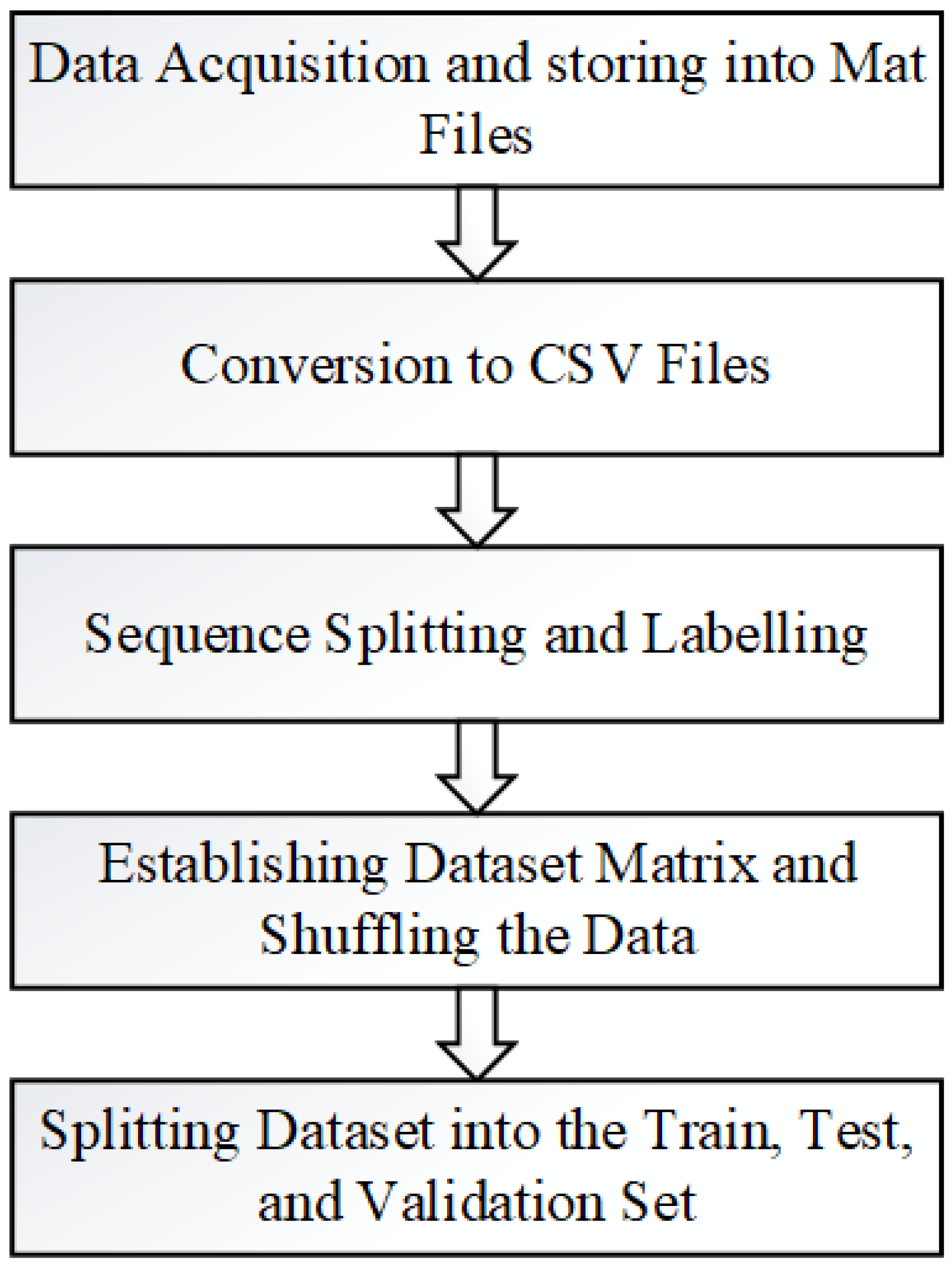
Therefore, it reduces the quantity of features and makes the convergence of the data-driven models simple and smooth. The acquired data are saved into comma-separated values (CSV) files and then pre-processed to form a structured dataset that is used for training the classification models. Labels are also assigned to the different classes of the dataset which are only assigned to the fully supervised models explored in this research. The main objective of this research is to explore a semi-supervised model, namely GAN, which only requires a subset of the labelled data to finetune its prediction capability. The dataset established in this research seems as shown in (23):

$$data=\left(\begin{array}{ccc}{\theta }_{11}& \dots & {\theta }_{1m}\\ ⋮& \dots & ⋮\\ {\theta }_{n1}& \dots & {\theta }_{nm}\\ 0& \dots & 6\end{array}\right)$$

(23)

where n represents the number of features that is 100 in a single sample of data during 0.63 s and m is the total number of examples of all the classes that is 3290 which includes 470 samples from each class. The last row includes the labels assigned to each class [0, 6].

The dataset was first segmented into fixed-length sequences prior to any shuffling or partitioning. Shuffling and splitting into training, validation, and test sets were performed at the sequence level, ensuring that raw time-series points or overlapping temporal segments were not shared across subsets. The selected sequence length of 100 samples (0.63 s) was determined through empirical evaluation, balancing classification performance with computational efficiency and response latency. While a formal sensitivity analysis across multiple sequence lengths was not conducted, preliminary testing indicated that shorter sequences reduced class separability, whereas longer sequences increased the prediction delay without significant performance gains. Figure 7 depicts the flow diagram of the dataset preparation.

4. Data-Driven Models and Performance Evaluation

In this section, we present the algorithms used for the investigation and evaluation of the metrics employed for the performance of various algorithms. The research is mainly based on a semi-supervised algorithm, namely GAN, while other supervised DL algorithms, namely MLP and 1D-CNN, are employed to compare the performance of the semi-supervised models. Each of these are discussed as follows.

4.1. Semi-Supervised Generative Adversarial Network

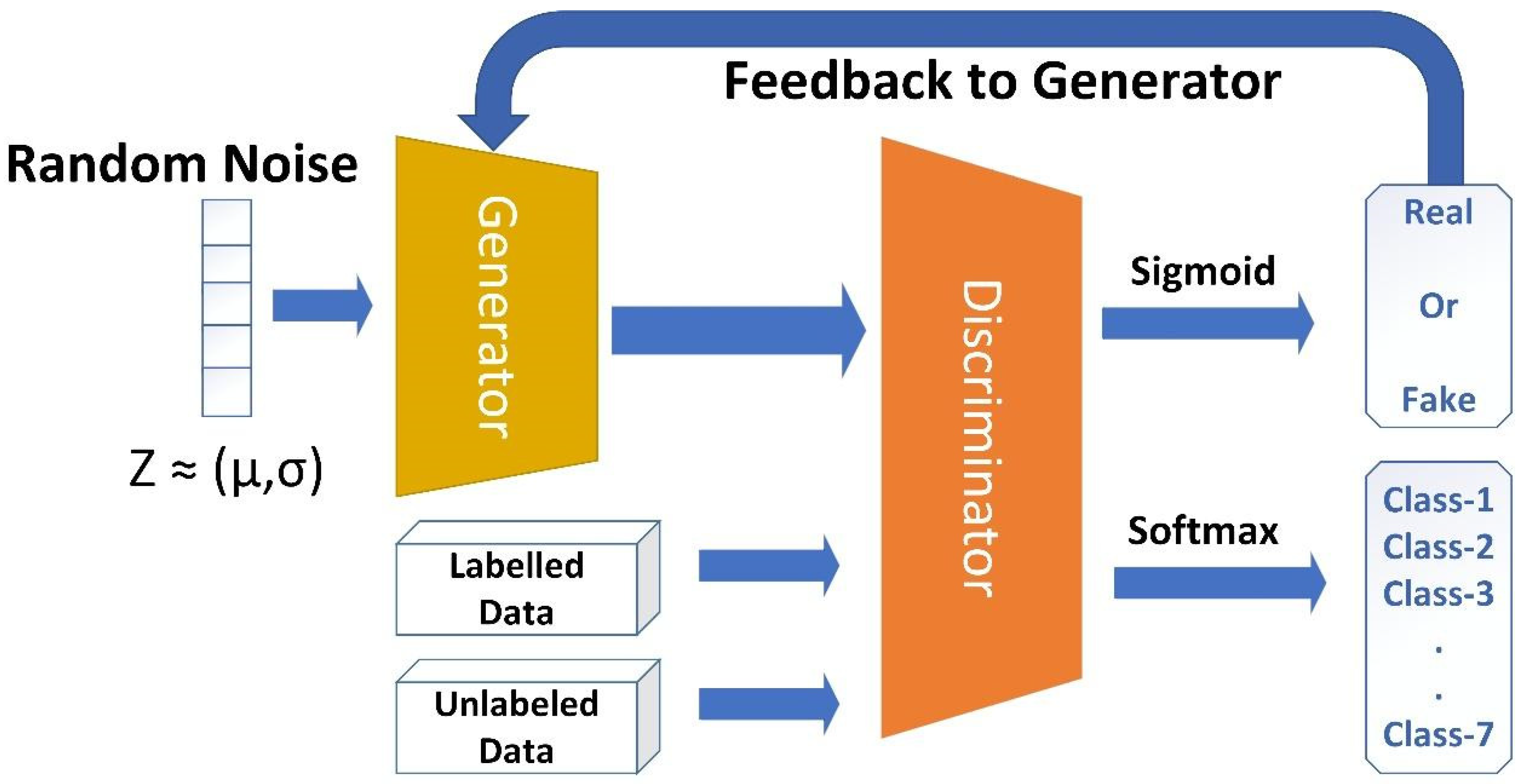
In general concept, a GAN [49] is a game theory-based algorithm. It comprises the two separate NN models including the Generator model (G-model) and Discriminator model (D-model) which are trained adversarial to improve the performance of the G-model. The G-model or D-model can be implemented through any NN topology such as MLP, DCNN or even auto-encoders. Figure 8 depicts the generalised architecture of a GAN model.

The main objective of the GAN architecture is to realise a G-model which can effectively generate samples which are indistinguishable from the actual examples. The G-model is inputted with a noise vector and then the generated data are fed to the D-model which predicts the class of the received data and whether they are real or fake. The optimisation technique of a GAN model is expressed by Equation (24):

$${\min }_G{\max }_{D}V(D,G)=E_{x-p_{data}}[\log D(x)]+E_{z-p_z(z)}[\log (1-D(G(z)))]$$

(24)

To learn the distribution of G-model P(data(x)), an input noise variable Pz (z) is specified. A mapping to latent space as G (z; θg) is provided where G represents a differentiable function mapped by a deep NN with parameter θg. The other deep NN D(x; θd) generates a single scalar. D(x) denotes the probability computed from the data rather than the variable Pg. The training of the D-model is performed to improve the probability of assigning the true labels to both the training samples and samples generated by the G-model. Moreover, in order to minimise log(1 − D(G(z))), both the G-model and D-model are trained simultaneously.

The goal behind the adversarial training of a semi-supervised GAN (SGAN) [50] is to have a discriminator with an added top layer and to optimise it for predicting the classes from the real data fed to the model. A semi-supervised GAN effectively performs the classification task with very few labelled samples. The D-model in a normal GAN yields an estimated probability that the input data are drawn from the data generating distribution. Conventionally, this model is implemented using a feed-forward network ending with a single sigmoid function. However, it can also be developed with a layer including a softmax function for predicting the classes [REAL, FAKE]. This modification allows the D-model to have N + 1 outputs corresponding to multiple classes. Figure 8 depicts the block diagram of the SGAN.

The architecture of the SGAN is almost similar to the GAN model but the SGAN is aimed at better classification performance with limited samples of labelled data. It seems clearly noticeable from the above architecture of the SGAN that the weights are shared between the classifier and discriminator, only the output units are separate for each. For GAN optimisation, the Adam optimiser was employed with an initial learning rate of 0.001. A learning rate scheduler was used to reduce the learning rate by a factor of 0.1 when the validation loss did not improve for five consecutive epochs. The categorical cross-entropy loss function was used for the classification task. Model convergence was monitored using validation loss stabilisation and classification performance, and training was terminated once no further improvement was observed.

The input data are organised as fixed-length sequential samples derived from directly measurable wheelset dynamics, including angular velocities, longitudinal velocity, and twist angle. Each sequence represents a single training instance for both the generator and discriminator–classifier networks. The SGAN architecture consists of two primary components: a generator trained to learn the underlying data distribution and produce synthetic feature representations, and a discriminator–classifier jointly optimised to distinguish real from generated samples while performing multiclass adhesion condition classification using both labelled and unlabelled data. This design enables effective representation learning under limited labelled data availability.

A noise vector with a certain number of samples is given as the input to the generator, and the same number of samples are fed from the real dataset. Subsequently, gradient descent is applied on both the discriminator and classifier. After that, more examples of the noise vector are taken and after that gradient descent is applied on the generator in response to the output generated by the discriminator and classifier. The model runs for a defined number of iterations until the desired classification results are obtained. It has been shown that the stochastic process of weight learning results in a more generalised model [50].

4.2. Comparative Deep Learning Models

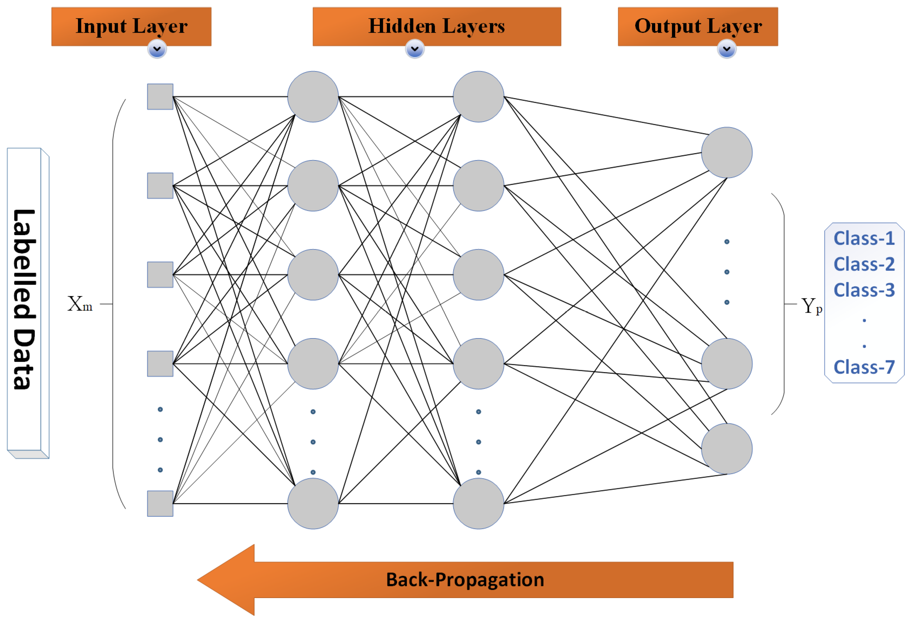
Since there has been very limited data-driven work on parameter estimation in wheel–rail contact, some baseline supervised algorithms are used first. Figure 9 depicts the structure of the MLP model employed in this research.

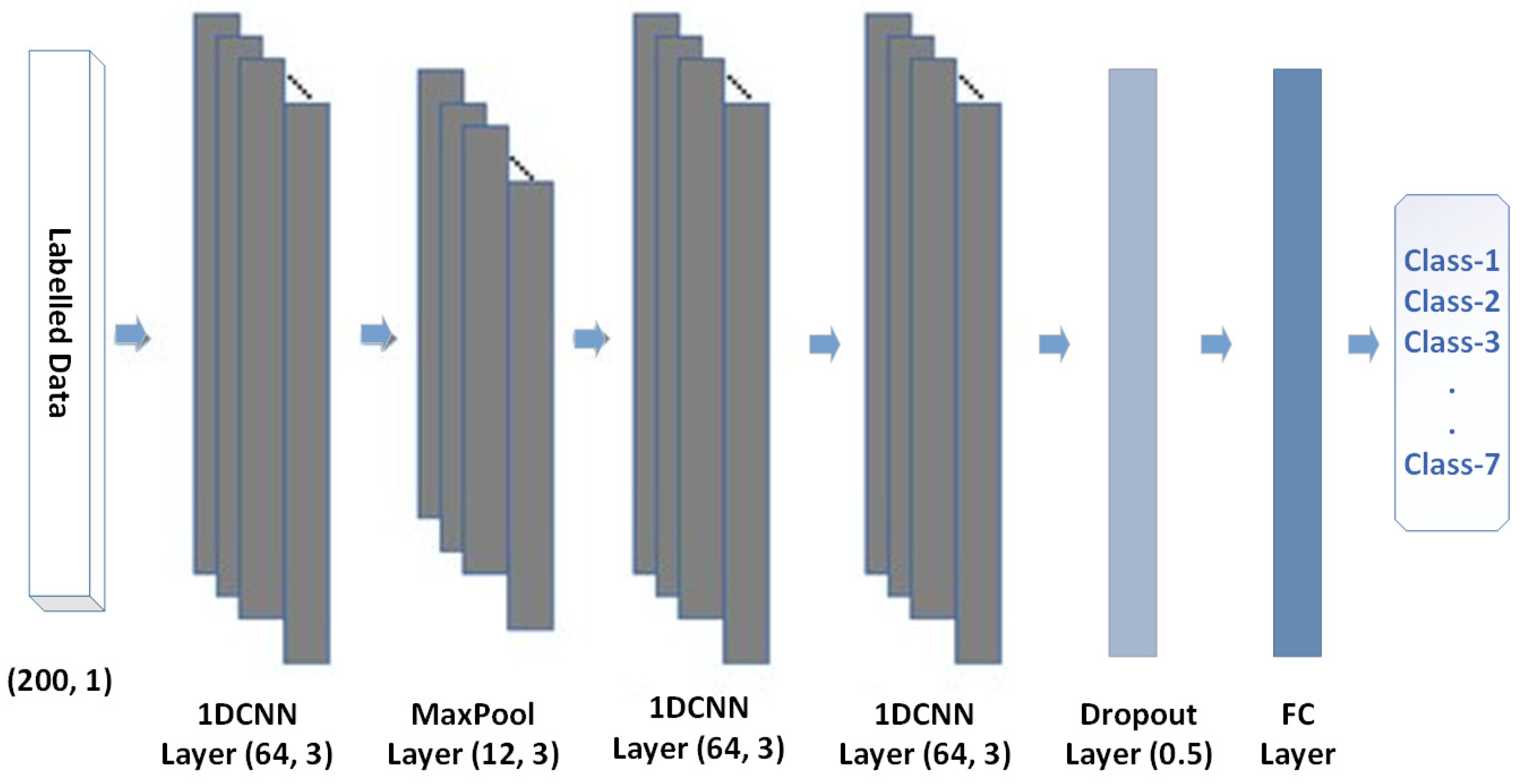
The MLP model comprises four densely connected layers each with 32 units with a RELU (rectifying linear unit) activation function. Categorical cross-entropy loss function is employed for the multiclass classification purpose. Softmax activation which is a stack of multiple sigmoid activation functions is added to the output layer and it yields the probability of each class. Similarly, the CNN model includes three 1D-CNN layers having rectified linear unit (RELU) activation functions. The model employs a pooling layer and dropout regularisation of 20% [51] to regularise the training process. Similar to the MLP model, softmax activation is added to the top of the model to compute the probabilities of the output classes. The architecture of the DCNN is depicted in Figure 10.

4.3. Experimental Configuration and Performance Evaluation of the Algorithms

The generalisation ability of a data-driven algorithm is evaluated by testing its prediction capabilities on unseen data samples [52]. The performance of DL models is evaluated using the following metrics: [53].

$$Accuracy={\displaystyle \frac{TN+TP}{TN+FP+TP+FN}}$$

(25)

$$\mathrm{Pr}ecision={\displaystyle \frac{TP}{TP+FP}}$$

(26)

$$\mathrm{Re}call={\displaystyle \frac{TP}{TP+FN}}$$

(27)

$$F1-score=2*{\displaystyle \frac{\mathrm{Pr}ecision*\mathrm{Re}call}{\mathrm{Pr}ecision+\mathrm{Re}call}}$$

(28)

where TP denotes true positives, TN denotes true negatives, FP denotes false positives, and FN denotes false negatives.

Moreover, to investigate these performance parameters various tools were used including the Simulink/Matlab (Version R2018a), GPU-based station (NVIDIA-1050ti GPU (NVIDIA Corporation, Santa Clara, CA, USA)), Python 3.7.1 (Anaconda Environment), Python libraries (Numpy, Pandas, and Scikit-learn), and DL frameworks (Keras and Tensorflow).

5. Results and Discussions

The wheelset model investigated in this study employs a pure conical wheel profile operating on a straight track at a fixed velocity, as described in the preceding section. The primary aim of this research is to implement and validate data-driven deep learning (DL) algorithms that can effectively learn from the variations in the lateral and yaw dynamics of the wheelset to accurately predict the adhesion conditions. Accordingly, directly measurable parameters were obtained from the simulated wheelset model, serving as the principal input features for the proposed data-driven framework.

5.1. Data Samples

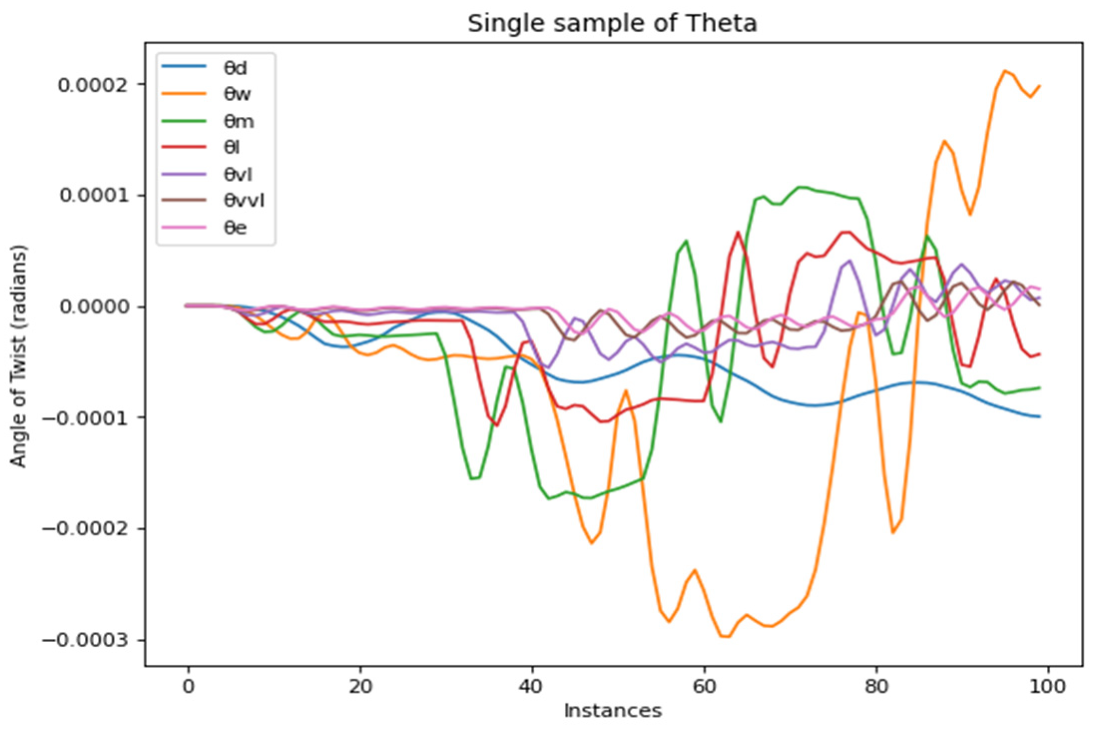
Figure 11 illustrates a single sample of the twist angle (θ), which represents the time-domain signal segment utilised by the DL models for adhesion-level classification. This feature captures the interaction dynamics between the wheel and rail, reflecting subtle variations in the adhesion regime. The small-amplitude oscillations in θ across instances highlight the non-linear and time-dependent nature of the contact interface, which the DL models are designed to interpret and classify effectively. Here, θ denotes the twist angle (as defined in Section 3.2), and the subscripts d, w, m, l, vl, vvl, and e correspond to dry, wet, medium adhesion, low adhesion, very low adhesion, very very low adhesion, and extremely low adhesion conditions, respectively.

5.2. Validation Results of Supervised Data-Driven Algorithms

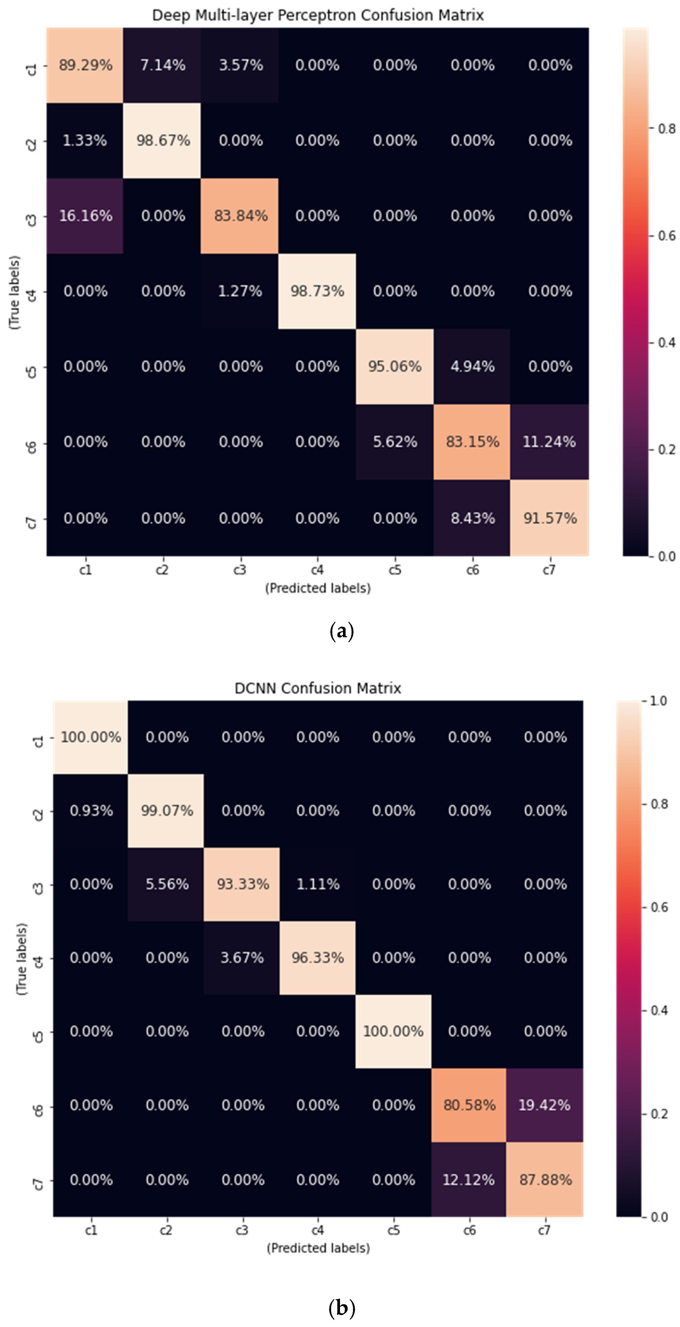
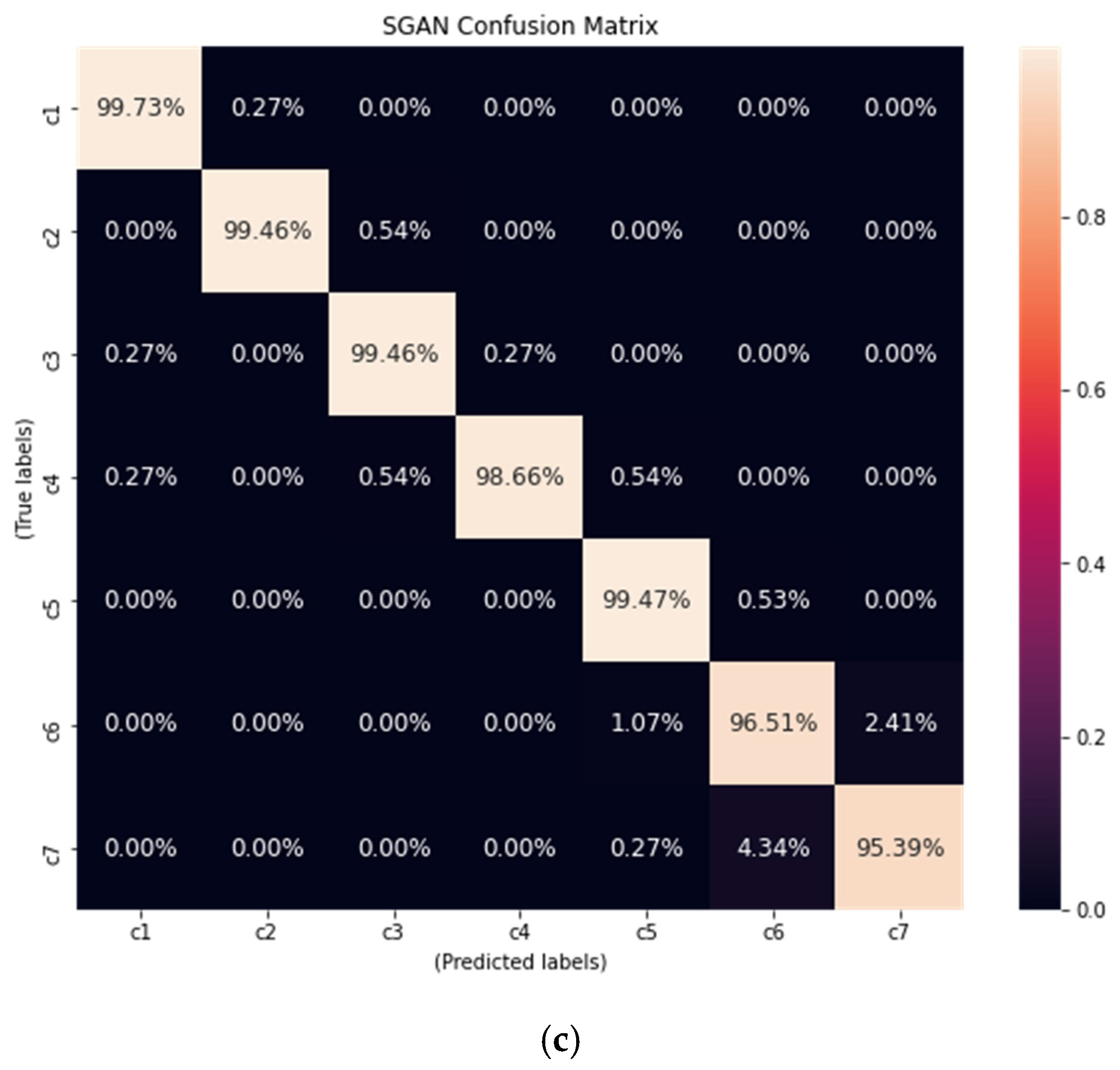
Initially, conventional supervised DL classifiers—Multilayer Perceptron (MLP) and 1D Convolutional Neural Network (1D-CNN)—were implemented to establish the baseline performance. Subsequently, a semi-supervised generative adversarial network (SGAN) was developed and trained using the same dataset to evaluate its ability to learn from both labelled and unlabelled data. The performance of these models, represented by the confusion matrices in Figure 12, demonstrates the classification accuracy for each adhesion condition.

The MLP model was able to differentiate between different adhesion conditions. All the classes were identified correctly with a testing accuracy greater than 90%, except three classes including C1, C2, and C6. The 1D-CNN outperformed the MLP, achieving an average cross-validation accuracy of 93.88%, demonstrating improved feature extraction from local temporal dependencies. However, its performance deteriorated in identifying extremely low adhesion conditions (C6), indicating a sensitivity to minor variations in the raw dynamic signals.

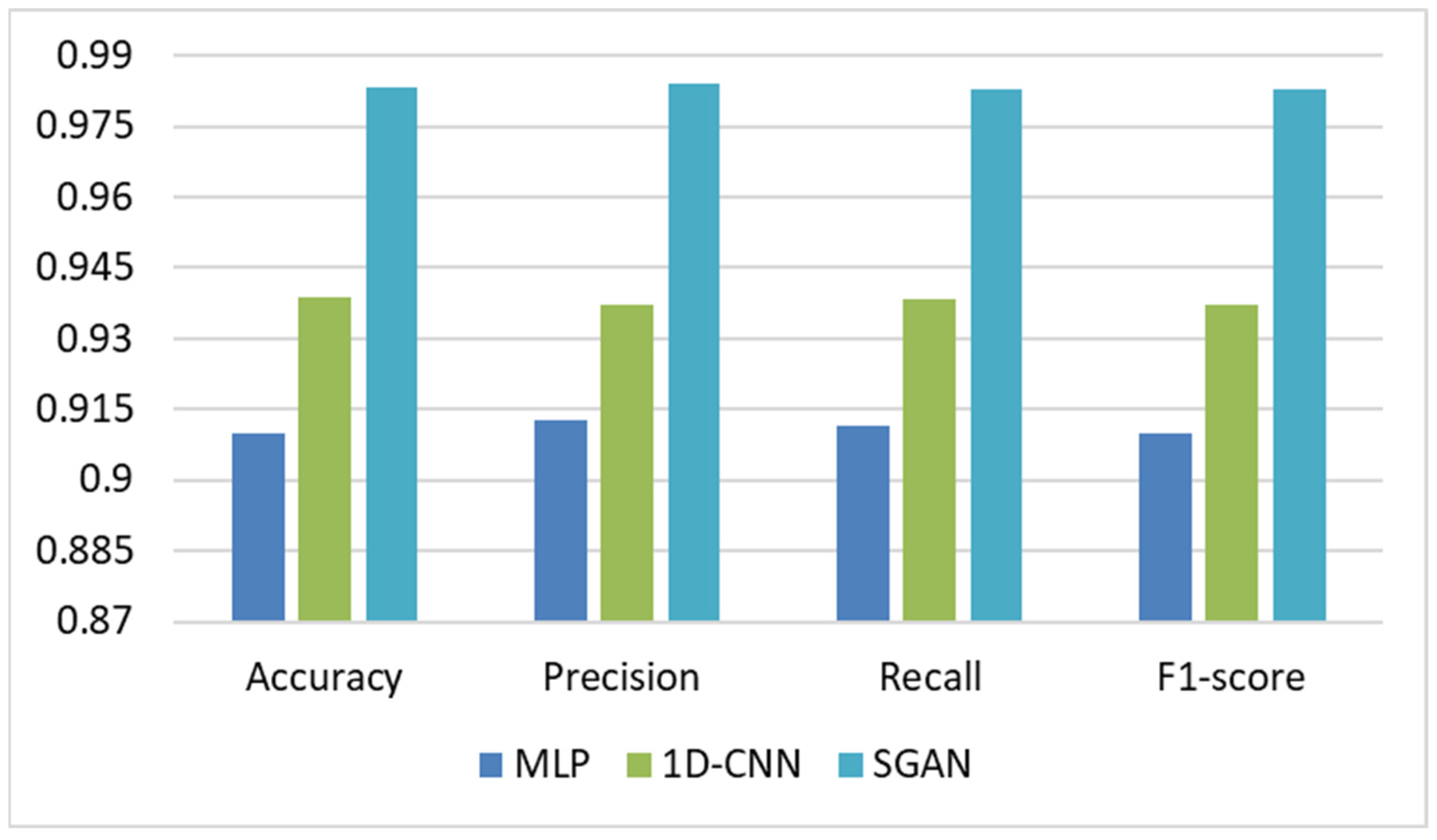
Figure 12c presents the confusion matrix of the SGAN classifier. The SGAN achieved an average class-wise accuracy above 98.38%, demonstrating exceptional robustness in distinguishing all seven adhesion levels. Remarkably, this performance was achieved using only fifty labelled samples, validating the model’s ability to leverage unlabelled data effectively through adversarial learning. Figure 13 summarises the comparative performance of all the models in terms of accuracy, precision, recall, and F1-score. SGAN consistently outperformed the supervised models across all evaluation metrics, whereas 1D-CNN surpassed MLP but remained below the SGAN benchmark.

5.3. Discussion

The results clearly indicate that semi-supervised learning significantly enhances adhesion-level identification in scenarios with limited labelled data—a common challenge in railway condition monitoring. Unlike supervised models that rely heavily on extensive, domain-labelled datasets, SGAN effectively captures the latent structure of adhesion-related dynamics through adversarial training, making it data-efficient and self-reliant.

Furthermore, SGAN’s ability to learn meaningful representations from raw, unlabelled sequences implies its suitability for real-time perception modules within intelligent and autonomous railway systems. The model’s performance demonstrates that data-driven algorithms can reliably replace traditional physics-based approaches in complex, non-linear contact problems such as wheel–rail adhesion.

Different operating conditions alter the underlying adhesion physics, which can lead to shifts in the input data distribution and, consequently, variations in the model performance. Depending on the operational regime, such distribution shifts may improve or degrade the prediction accuracy. While a unified data-driven model could be developed to handle multiple operating conditions, its effectiveness would depend on the availability of a dataset that spans a sufficiently wide range of speeds, loads, and rail surface conditions.

The proposed framework operates on directly measurable wheelset dynamics, such as angular velocities, longitudinal velocity, and twist angle, which can be acquired using onboard sensing systems. As a result, mapping to real-world conditions is achieved through these dynamic signals rather than through the explicit modelling of rail surface properties. Variations in the wheelset parameters, rail conditions, and operating environments are implicitly reflected in the measured responses. Validation under real-world noise, sensor imperfections, and environmental variability remains an important direction for future work.

From a computational perspective, SGAN training involves additional overhead due to adversarial optimisation and joint generator–discriminator updates. However, once training is completed, real-time inference relies solely on the discriminator–classifier network, resulting in low computational and memory requirements suitable for real-time deployment. A detailed quantitative benchmarking of training time and memory consumption across architectures is beyond the scope of the present study and is identified as a future work.

Though in this case study we have employed a GAN-based model as a possible solution in limited data scenarios, nonetheless, GAN-based models have several limitations. These types of DL architectures may suffer from training instability, which reduces diversity and makes convergence difficult and unpredictable. Furthermore, GAN-based models struggle to preserve fine-grained details and lack explicit likelihoods, making evaluation and uncertainty estimation difficult. Their performance is sensitive to dataset bias and may generalise poorly to out-of-distribution inputs. This research confirms that deep learning architectures, particularly SGAN, can be instrumental in developing adaptive, autonomous monitoring frameworks capable of continuous learning without manual labelling overhead. Such self-reliant systems hold potential for broader deployment across cyber–physical and robotic domains, where fault detection, predictive maintenance, and intelligent decision-making are critical for safe and efficient operation.

6. Conclusions

In this work, we have applied supervised and semi-supervised deep learning (DL) data-driven models to investigate adhesion estimation and compare their performance for the adhesion identification task. In the first step, a wheelset model was simulated, and data were acquired under different adhesion levels. Polach’s wheel–rail contact model was implemented to model the various adhesion conditions, and the wheelset model was subsequently operated under multiple adhesion regimes to analyse its dynamic response. Considering the goal of this research, directly measurable quantities, including angular velocities and their differences, were obtained to capture identifiable variations. The twist angle under different adhesion conditions was selected as a key training feature for the DL models, as it provided a scaled representation of both angular velocities. The generated dataset was used to train and test the supervised MLP and 1D-CNN models in MATLAB. The simulation results show that the MLP and 1D-CNN achieved average accuracies of 91% and 93%, respectively. Furthermore, the SGAN-based semi-supervised model effectively identified different adhesion classes with an accuracy of 98%, demonstrating its strong generalisation ability even with limited labelled data.

The proposed model demonstrates that adhesion-level identification and classification can be reliably achieved through self-reliant, data-driven DL architectures, which can serve as AI-based perception modules within intelligent and autonomous railway systems. To the best of our knowledge, this work represents one of the early studies investigating semi-supervised GAN-based adhesion condition identification using raw dynamic sequences, with a particular focus on low adhesion regimes under limited labelled data. This research contributes to the advancement of intelligent mobility by introducing a perception-driven framework capable of supporting decision-making in real time, like robotic perception and control mechanisms. The results confirm that semi-supervised architectures such as SGAN can bridge the gap between supervised learning and practical deployment in autonomous systems, providing both robustness and scalability for industrial applications.

Future work will focus on the validation of the proposed approaches within a multi-body simulation (MBS) environment and their subsequent real-time deployment in autonomous control architectures. Further extensions may include the integration of brake and traction condition models within intelligent railway or robotic mobility frameworks, along with the inclusion of sensor fusion techniques and edge-based learning to improve the perception accuracy and responsiveness in complex operating environments.

References

1. Iwnicki, S. Simulation of wheel-rail contact forces. Fatigue Fract. Eng. Mater. Struct. 2003, 26, 887–900. [Google Scholar] [CrossRef] [Scilit]
2. Mal, K.; Hussain, I.; Chowdhry, B.; Memon, T. Extended Kalman Filter for Estimation of Contact Forces at Wheel-Rail Interface. 3C Tecnol. 2020, 2020, 279–301. [Google Scholar] [CrossRef] [Scilit]
3. Olofsson, U.; Lewis, R. Tribology of the wheel-rail contact. In Handbook of Railway Vehicle Dynamics; CRC Press: Boca Raton, FL, USA, 2006; pp. 121–141. [Google Scholar]
4. Spiryagin, M.; Wolfs, P.; Wu, Q.; Cole, C.; Alahakoon, S.; Sun, Y.Q.; McSweeney, T.; Spiryagin, V. Rail cleaning process and its influence on locomotive performance. In Proceedings of the 2017 Joint Rail Conference, Philadelphia, PA, USA, 4–7 April 2017. [Google Scholar]
5. Mal, K.; Hussain, I.; Memon, T.; Kumar, D.; Chowdhry, B. Modern Condition Monitoring Systems for Railway Wheel-Set Dynamics: Performance Analysis and Limitations of Existing Techniques. Sir Syed Univ. Res. J. Eng. Technol. 2022, 12, 31–41. [Google Scholar] [CrossRef] [Scilit]
6. Olofsson, U.; Lyu, Y. Open system tribology in the wheel-rail contact—A literature review. Appl. Mech. Rev. 2017, 69, 060802. [Google Scholar] [CrossRef] [Scilit]
7. Shrestha, S.; Wu, Q.; Spiryagin, M. Review of adhesion estimation approaches for rail vehicles. Int. J. Rail Transp. 2019, 7, 79–102. [Google Scholar] [CrossRef] [Scilit]
8. Hubbard, P.; Harrison, T.; Ward, C.; Abduraxman, B. Creep slope estimation for assessing adhesion in the wheel/rail contact. IET Intell. Transp. Syst. 2024, 18, 1931–1942. [Google Scholar] [CrossRef] [Scilit]
9. Mal, K. FPGA-Based Railway Wheelset Parameters Estimation Using Kalman Filter. Ph.D. Thesis, Mehran University of Engineering and Technology, Jamshoro, Pakistan, 2023. [Google Scholar]
10. Mal, K.; Kalwar, I.H.; Shaikh, K.; Memon, T.D.; Chowdhry, B.S.; Nisar, K.; Gupta, M. A new estimation of nonlinear contact forces of railway vehicle. Intell. Autom. Soft Comput. 2021, 28, 823–841. [Google Scholar] [CrossRef] [Scilit]
11. Alahakoon, S.; Sun, Y.; Spiryagin, M.; Cole, C. Rail flaw detection technologies for safer, reliable transportation: A review. J. Dyn. Syst. Meas. Control 2018, 140, 823–841. [Google Scholar] [CrossRef] [Scilit]
12. Kumar, D.; Daudpoto, J.; Harris, N.; Hussain, M.; Mehran, S.; Kalwar, I.H.; Hussain, T.; Memon, T.D. The Importance of Feature Processing in Deep-Learning-Based Condition Monitoring of Motors. Math. Probl. Eng. 2021, 2021, 9927151. [Google Scholar] [CrossRef] [Scilit]
13. Li, C.; Luo, S.; Cole, C.; Spiryagin, M. An overview: Modern techniques for railway vehicle on-board health monitoring systems. Veh. Syst. Dyn. 2017, 55, 1045–1070. [Google Scholar] [CrossRef] [Scilit]
14. Garg, V. Dynamics of Railway Vehicle Systems; Elsevier: Amsterdam, The Netherlands, 2012. [Google Scholar]
15. Mal, K.; Memon, T.; Hussain, I.; Chowdhry, B. FPGA Implementation of Extended Kalman Filter for Parameters Estimation of Railway Wheelset. Comput. Mater. Contin. 2023, 74, 3351–3370. [Google Scholar] [CrossRef] [Scilit]
16. Onat, A.; Voltr, P.; Lata, M. A new friction condition identification approach for wheel-rail interface. Int. J. Rail Transp. 2017, 5, 127–144. [Google Scholar] [CrossRef] [Scilit]
17. Mal, K.; Chowdhry, B.; Kalwar, I.; Memon, T. Performance Analysis of FPGA-Based Extended Kalman Filter for Railway Wheelset Parameters Estimation. In Proceedings of the Sixth International Conference on Railway Technology: Research, Development and Maintenance; Civil-Comp Press: Edinburgh, UK, 2024; Volume 7, Paper 7.5. [Google Scholar] [CrossRef] [Scilit]
18. Hussain, I.; Mei, T.; Ritchings, R. Estimation of wheel-rail contact conditions and adhesion using the multiple model approach. Veh. Syst. Dyn. 2013, 51, 32–53. [Google Scholar] [CrossRef] [Scilit]
19. Pichlík, P.; Zděnek, J. Adhesion force detection method based on the Kalman filter for slip control purpose. Automatika 2016, 57, 405–415. [Google Scholar] [CrossRef]
20. Pichlík, P.; Zděnek, J. Comparison of locomotive adhesion force estimation methods for a wheel slip control purpose. In 9th International Conference on Electronics, Computers and Artificial Intelligence (ECAI); IEEE: Piscataway, NJ, USA, 2017. [Google Scholar]
21. Zhao, Y.; Liang, B. Re-adhesion control for a railway single wheelset test rig based on the behavior of the traction motor. Veh. Syst. Dyn. 2013, 51, 1173–1185. [Google Scholar] [CrossRef] [Scilit]
22. Zhao, Y.; Liang, B.; Iwnicki, S. Friction coefficient estimation using an unscented Kalman filter. Veh. Syst. Dyn. 2014, 52, 220–234. [Google Scholar] [CrossRef] [Scilit]
23. Charles, G.; Goodall, R.; Dixon, R. Model-based condition monitoring at the wheel-rail interface. Veh. Syst. Dyn. 2008, 46, 415–430. [Google Scholar] [CrossRef] [Scilit]
24. Allota, B.; Malvezzi, M.; Toni, P. Adhesion models for wheel/rail contact in railways. In Proceedings of the 2nd World Tribology Congress, Vienna, Austria, 3–7 September 2001. [Google Scholar]
25. Meli, E.; Ridolfi, A. An innovative wheel-rail contact model for railway vehicles under degraded adhesion conditions. Multibody Syst. Dyn. 2015, 33, 285–313. [Google Scholar] [CrossRef] [Scilit]
26. Strano, S.; Terzo, M. On the real-time estimation of the wheel-rail contact force by means of a new nonlinear estimator design model. Mech. Syst. Signal Process. 2018, 105, 391–403. [Google Scholar] [CrossRef] [Scilit]
27. Ward, C.; Goodall, R.; Dixon, R.; Charles, G.A. Adhesion estimation at the wheel-rail interface using advanced model-based filtering. Veh. Syst. Dyn. 2012, 50, 1797–1816. [Google Scholar] [CrossRef] [Scilit]
28. Kalman, R. A new approach to linear filtering and prediction problems. Trans. ASME–J. Basic Eng. 1960, 82, 35–45. [Google Scholar] [CrossRef] [Scilit]
29. Pichlík, P.; Zděnek, J. Extended Kalman filter utilization for a railway traction vehicle slip control. In International Conference on Optimization of Electrical and Electronic Equipment (OPTIM) & Intl Aegean Conference on Electrical Machines and Power Electronics (ACEMP); IEEE: Piscataway, NJ, USA, 2017. [Google Scholar]
30. Shim, J.; Koo, J.; Park, Y. A Methodology of Condition Monitoring System Utilizing Supervised and Semi-Supervised Learning in Railway. Sensors 2023, 23, 9075. [Google Scholar] [CrossRef] [Scilit]
31. Balogun, I.; Attoh-Okine, N. Covariate-Shift Generative Adversarial Network and Railway Track Image Analysis. J. Transp. Eng. Part A Syst. 2023, 149, 04022158. [Google Scholar] [CrossRef] [Scilit]
32. Raza, A.; Sehar, R.; Moiz, A.; Alluhaidan, A.S.; El-Rahman, S.A.; AbdElminaam, D.S. Novel conditional tabular generative adversarial network based image augmentation for railway track fault detection. PeerJ Comput. Sci. 2025, 11, e2898. [Google Scholar] [CrossRef] [Scilit]
33. Gajdar, T.; Rudas, I.; Suda, Y. Neural network based estimation of friction coefficient of wheel and rail. In Proceedings of IEEE International Conference on Intelligent Engineering Systems; IEEE: Piscataway, NJ, USA, 1997. [Google Scholar]
34. Falomi, S.; Malvezzi, M.; Meli, E.; Rindi, A. Determination of wheel-rail contact points: Comparison between classical and neural network based procedures. Meccanica 2009, 44, 661–686. [Google Scholar] [CrossRef] [Scilit]
35. Malvezzi, M.; Pugi, L.; Papini, S.; Rindi, A.; Toni, P. Identification of a wheel-rail adhesion coefficient from experimental data during braking tests. Proc. Inst. Mech. Eng. Part F J. Rail Rapid Transit 2013, 227, 128–139. [Google Scholar] [CrossRef] [Scilit]
36. Li, N.; Feng, X.; Wei, X. Optimized adhesion control of locomotive airbrake based on GSA-RNN. In 7th International Conference on Intelligent Human-Machine Systems and Cybernetics; IEEE: Piscataway, NJ, USA, 2015. [Google Scholar]
37. Castillo, J.; Cabrera, J.; Guerra, A.; Simón, A. A novel electrohydraulic brake system with tire-road friction estimation and continuous brake pressure control. IEEE Trans. Ind. Electron. 2015, 63, 1863–1875. [Google Scholar] [CrossRef] [Scilit]
38. Han, K.; Wang, Y. Research on a Lightweight Rail Surface Condition Identification Method for Wheel–Rail Maximum Adhesion Coefficient Estimation. Appl. Sci. 2025, 15, 3391. [Google Scholar] [CrossRef] [Scilit]
39. He, J.; Liu, L.; Zhang, C.; Zhao, K.; Sun, J.; Li, P. Deep denoising autoencoding method for feature extraction and recognition of vehicle adhesion status. J. Sens. 2018, 2018, 5419645. [Google Scholar] [CrossRef] [Scilit]
40. Zhang, C.; Cheng, X.; Liu, J.; He, J.; Liu, G. Deep sparse autoencoder for feature extraction and diagnosis of locomotive adhesion status. J. Control Sci. Eng. 2018, 2018, 8676387. [Google Scholar] [CrossRef] [Scilit]
41. Liu, J.; Liu, L.; He, J.; Zhang, C.; Zhao, K. Wheel/rail adhesion state identification of heavy-haul locomotive based on particle swarm optimization and kernel extreme learning machine. J. Adv. Transp. 2020, 2020, 8136939. [Google Scholar] [CrossRef] [Scilit]
42. Ujjan, S.; Hussain, I.; Chowdhry, B.; Memon, T.D.; Soother, D.K. Adhesion level identification in wheel-rail contact using deep neural net-works. 3C Tecnol. 2020, 217–231. [Google Scholar] [CrossRef] [Scilit]
43. Johansson, A.; Nielsen, J. Out-of-round railway wheels-wheel-rail contact forces and track response derived from field tests and numerical simulations. Proc. Inst. Mech. Eng. Part F J. Rail Rapid Transit 2003, 217, 135–146. [Google Scholar] [CrossRef] [Scilit]
44. Yu, J.; Mei, T.; Wilson, D. Re-adhesion control based on wheelset dynamics in railway traction system. In Proceedings of the UKACC International Control Conference on Control, Glasgow, UK, 30 August–1 September 2006. [Google Scholar]
45. Park, K.; Lee, H.; Park, C.; Kim, D.; Lee, M. The characteristics of deriving control of crane [deriving read driving]. In IEEE International Symposium on Industrial Electronics Proceedings (Cat. No. 01TH8570); IEEE: Piscataway, NJ, USA, 2001. [Google Scholar]
46. Kalker, J. The computation of three dimensional rolling contact with dry friction. Int. J. Numer. Methods Eng. 1979, 14, 1293–1307. [Google Scholar] [CrossRef] [Scilit]
47. Thompson, D. Fundamentals of Rail Vehicle Dynamics: Guidance and Stability. Proc. Inst. Mech. Eng. 2004, 218, 265. [Google Scholar] [CrossRef] [Scilit]
48. Polach, O. Characteristic parameters of nonlinear wheel/rail contact geometry. Veh. Syst. Dyn. 2010, 48, 19–36. [Google Scholar] [CrossRef] [Scilit]
49. Goodfellow, I.; Pouget-Abadie, J.; Mirza, M.; Xu, B.; Warde-Farley, D.; Ozair, S.; Courville, A.; Bengio, Y. Generative adversarial nets. In Proceedings of the Advances in Neural Information Processing Systems, Montreal, QC, Canada, 8–13 December 2014. [Google Scholar]
50. Odena, A. Semi-supervised learning with generative adversarial networks. arXiv 2016, arXiv:1606.01583. [Google Scholar]
51. Srivastava, N.; Hinton, G.; Krizhevsky, A.; Sutskever, I.; Salakhutdinov, R. Dropout: A simple way to prevent neural networks from overfitting. J. Mach. Learn. Res. 2014, 15, 1929–1958. [Google Scholar]
52. Goodfellow, I.; Bengio, Y.; Courville, A. Deep Learning; MIT Press: Cambridge, MA, USA, 2016; Volume 1. [Google Scholar]
53. Soother, D.K.; Kalwar, I.H.; Hussain, T.; Chowdhry, B.S.; Ujjan, S.M.; Memon, T.D. A Novel Method Based on UNET for Bearing Fault Diagnosis. Comput. Mater. Contin. 2021, 69, 393–408. [Google Scholar] [CrossRef] [Scilit]
Figure 1. A solid axle wheelset.
Ai 07 00078 g001
Figure 2. Longitudinal velocity response under different adhesion levels.
Ai 07 00078 g002
Figure 3. Twist angle response under different adhesion levels.
Ai 07 00078 g003
Figure 4. Angular velocity of the left wheel under different adhesion levels.
Ai 07 00078 g004
Figure 5. Angular velocity of the right wheel under different adhesion levels.
Ai 07 00078 g005
Figure 6. Adhesion conditions used in the simulation study, defined based on the adhesion coefficient (μ, dimensionless), ranging from high to extremely low adhesion levels. The labels C1–C7 correspond to dry (C1), wet (C2), medium adhesion (C3), low adhesion (C4), very low adhesion (C5), very very low adhesion (C6), and extremely low adhesion (C7) conditions.
Ai 07 00078 g006
Figure 7. Flow chart of dataset preparation.
Ai 07 00078 g007
Figure 8. SGAN architecture implemented.
Ai 07 00078 g008
Figure 9. Structure of MLP model.
Ai 07 00078 g009
Figure 10. Structure of the 1D-CNN model.
Ai 07 00078 g010
Figure 11. Single sample of angle of twist.
Ai 07 00078 g011
Figure 12. Confusion matrices of (a) MLP, (b) 1D-CNN, and (c) SGAN.
Ai 07 00078 g012aAi 07 00078 g012b
Figure 13. Evaluation summary of the DL models.
Ai 07 00078 g013