Article

Should We Reconsider RNNs for Time-Series Forecasting?

by
Vahid Naghashi
1,2,
Mounir Boukadoum
1,2 and
Abdoulaye Banire Diallo
1,2,*
1
Department of Computer Science, Université du Québec à Montréal, Montreal, QC H2L 2C4, Canada
2
WELL-E: Research and Innovation Chair in Animal Welfare and Artificial Intelligence, Montreal, QC H2L 2C4, Canada
*
Author to whom correspondence should be addressed.
Submission received: 2 April 2025 / Revised: 23 April 2025 / Accepted: 24 April 2025 / Published: 25 April 2025
(This article belongs to the Section AI Systems: Theory and Applications)

Abstract

:
(1) Background: In recent years, Transformer-based models have dominated the time-series forecasting domain, overshadowing recurrent neural networks (RNNs) such as Long Short-Term Memory (LSTM) and Gated Recurrent Unit (GRU). While Transformers demonstrate superior performance, their high computational cost limits their practical application in resource-constrained settings. (2) Methods: In this paper, we reconsider RNNs—specifically the GRU architecture—as an efficient alternative to time-series forecasting by leveraging this architecture’s sequential representation capability to capture cross-channel dependencies effectively. Our model also utilizes a feed-forward layer right after the GRU module to represent temporal dependencies, and aggregates it with the GRU layers to predict future values of a given time-series. (3) Results and conclusions: Our extensive experiments conducted on different real-world datasets show that our inverted GRU (iGRU) model achieves promising results in terms of error metrics and memory efficiency, challenging or surpassing state-of-the-art models on various benchmarks.

1. Introduction

Time-series forecasting is an important task in several application domains, including finance, meteorology, transportation, and energy consumption. Providing accurate forecasts helps industries and businesses save both money and time by enabling optimized and informed decision-making ahead of time, thereby avoiding unnecessary actions. Time-series forecasting involves leveraging historical (past) data from various channels or variates to predict future values of the same or related variates. As shown in Figure 1, these variables are often inter-correlated, and temporal relationships exist along the time dimension in a time-series. Time-series analysis and forecasting have garnered significant attention from researchers over the past few decades. With the rise of Artificial Intelligence (AI), deep learning-based methods have taken the lead in this field [1]. Among the deep learning models developed for time-series forecasting, Recurrent Neural Networks (RNNs), Convolutional Neural Networks (CNNs), Multi-Layer Perceptrons (MLPs), Transformer models, and Large Language Model (LLM)-based approaches have attained remarkable performance due to their ability to capture complex long-term temporal dependencies [1,2,3,4,5]. A model usually demonstrates high performance for multivariate time-series forecasting when it captures the relations between the prediction variables and the temporal correlations across the historical time steps. There are two main approaches used for time-series forecasting with deep learning models. The first category of methods are known as Channel-Dependent (CD) methods, which usually project the channel dimension into a hidden space (modeling dimension). However, recent works have shown that Channel-Independent (CI) models generally achieve better results [6,7]. Recently, many Transformer-based models have been proposed using channel independence, where multiple channels are predicted independently. In addition, one of the recently invented CI-based models, iTransformer [8], directly captures the intricate interaction among multiple time-series channels by exploiting the high capacity of the multi-head self-attention module inside the Transformer, and embedding the temporal dimension within the model dimension, leading to impressive results, specifically when dealing with complex real-world datasets. However, the Transformer-based models face the obvious challenge of quadratic time complexity with respect to the input sequence length, specifically in the inference step, which gives rise to an intensive calculation when applied to a large number of variates or longer look-back windows, hindering their deployment in real-world applications.
There have already been attempts to reduce the computational complexity of Transformer for time-series forecasting. For instance, Ref. [9] modified the Transformer to focus on a portion of the sequence, while other works utilized linear models to decrease the time complexity [7,10]. Although linear models can reduce time complexity, they mainly rely on linear computations and fail to exploit contextual information, resulting in sub-optimal predictions, specifically when applied to datasets involving many variates or series. Given the prevalent use of Transformer models in the time-series forecasting (TSF) domain, recurrent models such as LSTM and GRU have been neglected and their potential to capture cross-channel dependencies escaped the attention of researchers in the field. RNNs are still occasionally utilized for TSF [11] in rare cases. However, their capability for sequential modeling is underestimated compared to that of Transformers.
In this paper, we reconsider the RNNs, specifically the Gated Recurrent Unit (GRU), as an alternative to the multi-head self-attention module in the Transformer models. We exploit GRUs to extract the interactions among time-series channels and utilize them in multiple-channel forecasting. Inspired by the iTransformer [8] model, we apply the GRU to the channel dimension of the input series to capture inter-series correlations. Considering the importance of capturing cross-channel correlations in time-series analysis, we will answer the question of whether RNNs (including GRU or LSTM) should still be considered for time-series forecasting. We answer this question by conducting experiments using various public time-series datasets and analyzing the results, specifically through the ablation experiments. Recurrent Neural Networks (RNNs) represent significant advantages in inference time efficiency for time-series forecasting, although their performance sometimes falls behind that of Transformer-based architectures. The proposed iGRU achieves a competitive performance with reduced computational overhead. On datasets like Solar, iGRU outperforms several Transformer models in both accuracy and efficiency, as shown in Section 3. However, for some datasets, iGRU’s performance is surpassed by computation-intensive models, reflecting a trade-off between accuracy and computational cost. This work explores these trade-offs, demonstrating iGRU’s potential as a lightweight and effective model for time-series forecasting task. Furthermore, in most cases, iGRU outperforms the recently proposed iTransformer [8]. The prominent reason for utilizing GRUs in our model is that RNNs provide significantly lower time and memory complexity compared to many Transformer-based models, resulting in improved efficiency for specific applications, as demonstrated in Table 1. Additionally, the clear temporal flow in RNNs provides better interpretability in understanding how information propagates through sequences [12], specifically when compared to Transformer and MLP-based architectures.
Our work includes the following contributions to the time-series forecasting domain:
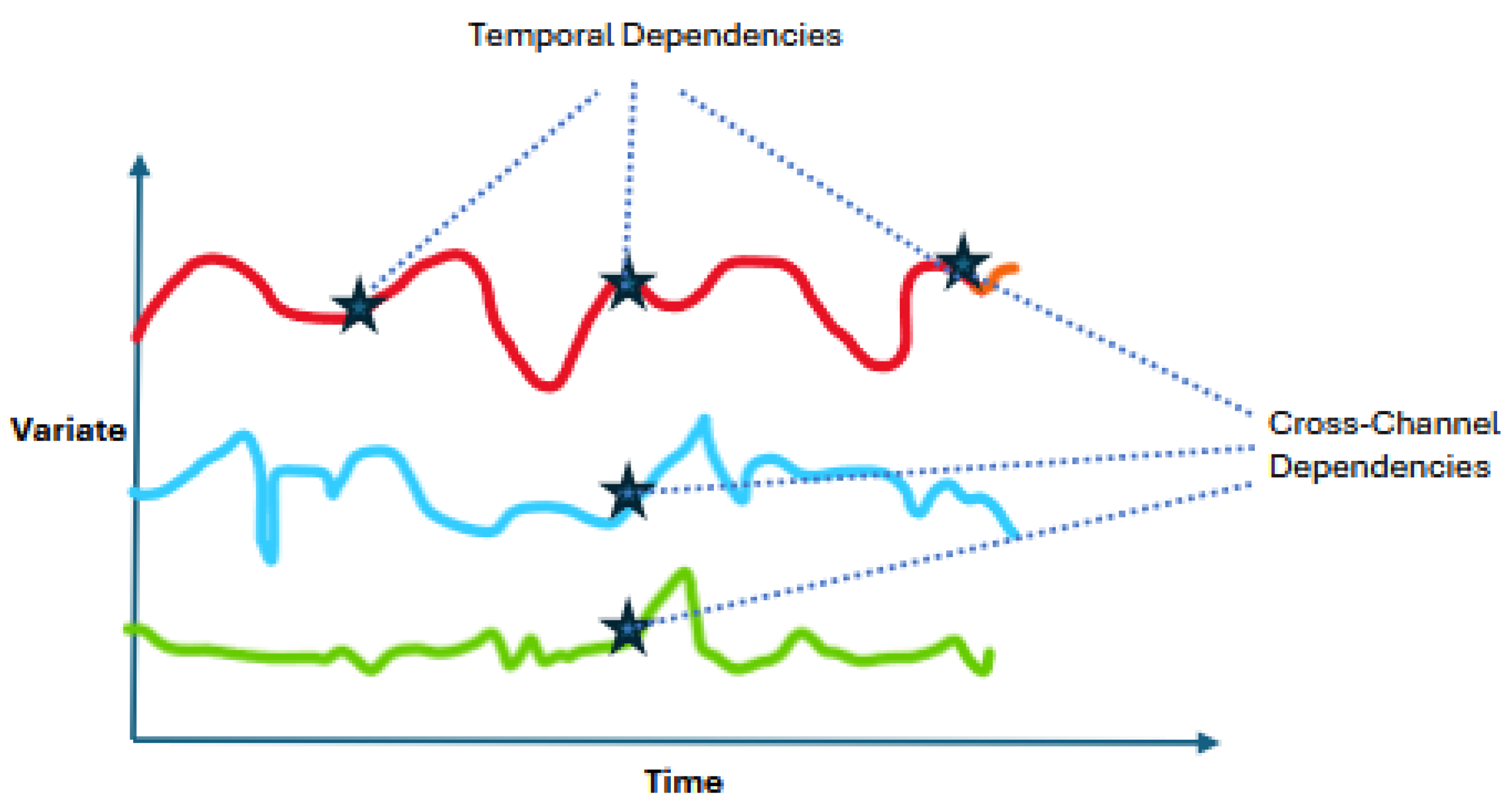
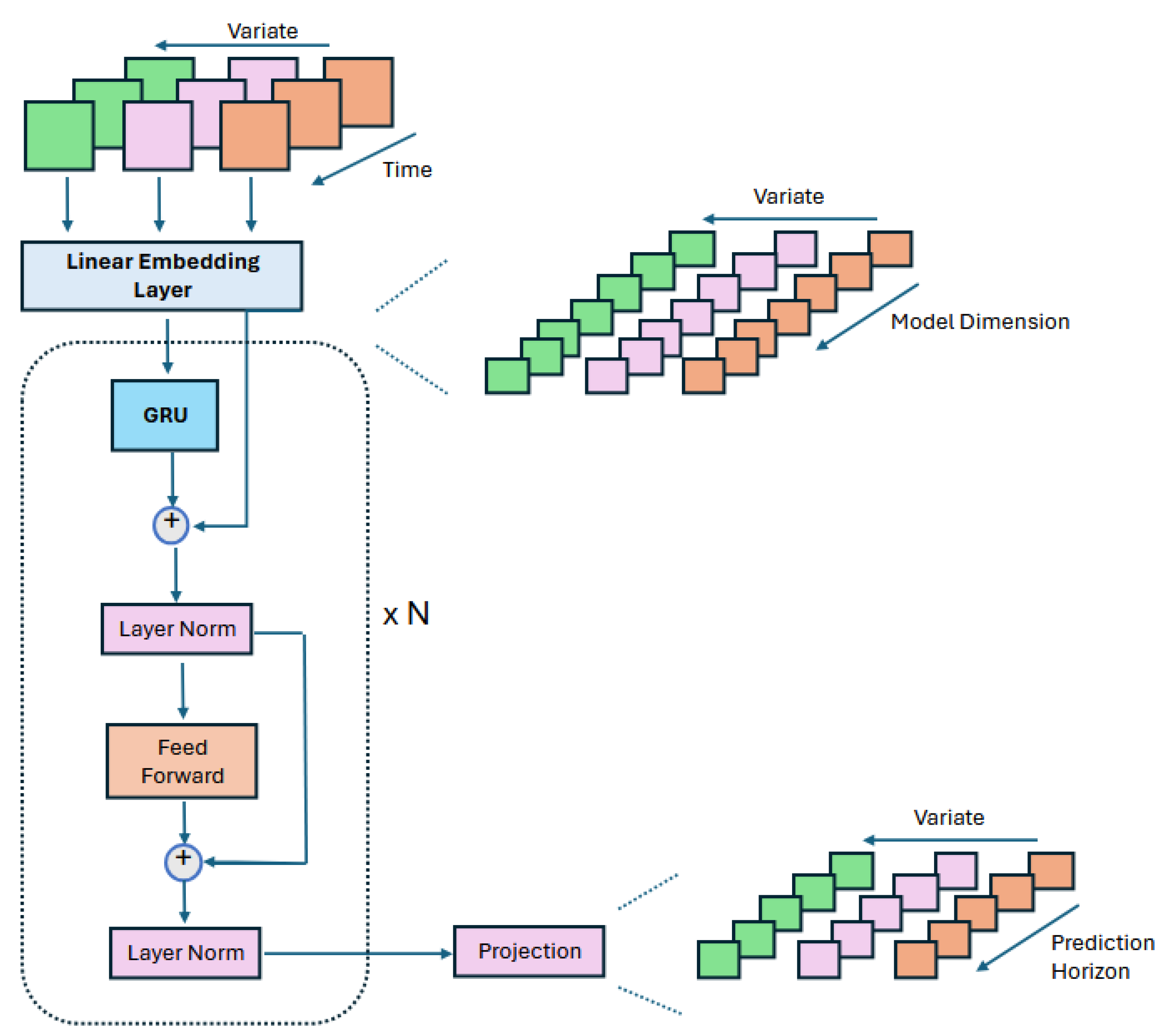
  • We reconsider RNNs for time-series forecasting using a different approach by focusing on the inter-channel dependencies and describe the inverted GRU (iGRU), which exploits GRU blocks to capture interactions between the time-series channels and feed-forward layers to represent temporal relations.
  • We extensively evaluate iGRU on eleven public datasets and report the results in terms of error metrics and memory efficiency.
  • We show that our iGRU model achieves comparable results to the state-of-the-art models or outperforms them.
Time-series forecasting methods are generally categorized into statistical models, such as Auto-ARIMA [13], and modern (deep learning) approaches, including Transformer, linear and convolutional neural network models. The Transformer architecture was initially designed to process and generate token sequences, mainly for natural language processing applications, especially Large Language Models (LLMs). However, its excellent potential motivated the TSF research community to deploy and adapt it for time-series tasks. For instance, LogTrans [14] uses convolutional attention in the LogSparse design to capture local information and reduce time complexity. The Informer [15] exploits the ProbSparse self-attention with distillation to emphasize prominent keys. In the Autoformer [16], the idea of time-series decomposition and auto-correlation calculation is proposed to extract temporal correlations. The FEDformer [17] is designed based on Fourier-based architecture and achieves a linear time complexity. In another work, the Pyraformer [18] utilizes pyramidal attention to capture inter-scale and intra-scale relations with a linear complexity. Recently, PatchTST [19] was proposed based on a Transformer architecture, which utilizes patched time-series with channel independence to capture temporal correlations for each channel, separately. In a different design, the Crossformer [20] exploits an encoder–decoder structure with hierarchical attention modules to leverage cross-channel dependencies. However, some Linear models have emerged recently to outperform Transformers in benchmark experiments [7,21]. On the other hand, these linear models fall short in representing non-linear dependencies between the input series and future time steps [7]. Recently, CNN-based models achieved promising results in time-series analysis tasks. As a prominent example, TimesNet [22] utilizes two-dimensional convolutions to capture inter-period and intra-period relations in a time-series with multiple period lengths, obtaining promising results. Over the past few years, Transformers and CNNs have overshadowed Recurrent Neural Networks (RNNs) in the time-series forecasting domain. For instance, the iTransformer [8] model is proposed based on the vanilla Transformer model and embedding the channels of the input series. This model attained impressive results in many benchmark datasets, pinpointing the importance of modeling cross-channel interactions in the forecasting tasks. The more recent model, TimeXer [23], incorporates the external information to enhance the forecasting accuracy, which strengthens the canonical Transformer to harmonize endogenous and exogenous information by using patch-wise self-attention and cross-variate attention, simultaneously. In this paper, we reconsider the potential of RNNs for capturing sequential dependencies and introduce the inverted GRU (iGRU), which leverages GRUs to capture dependencies across time-series channels while utilizing feed-forward layers to extract temporal features.

2. Materials and Methods

Our iGRU architecture is illustrated in Figure 2 and the corresponding forecasting procedure is shown in Algorithm 1. Given x t R C , the observation of a time-series with C channels at time t, we aim to forecast its future H time-steps x t + 1 , . . . , x t + H using a history or context window w t of length L (i.e., w t = ( x t L + 1 , . . . , x t ) ).
Algorithm 1 The forecasting procedure of iGRU
Input: Batch ( X ) = [ x 1 , x 2 , , x L ] : ( B , L , C )
Output: Batch ( Y ) = [ y 1 , y 2 , , y H ] : ( B , H , C )
  1:
X T : ( B , C , L ) Transpose ( Batch ( X ) )
  2:
X e m b e d d e d : ( B , C , D ) Embedding ( X T )
  3:
for each layer l in iGRU layers do
  4:
    X C C GRU ( X e m b e d d e d )
  5:
    X C C R X C C + X e m b e d d e d
  6:
    X C C R LayerNorm ( X C C R )
  7:
    X F F Feed - Forward ( X C C R )
  8:
    X F F X F F + X C C R
  9:
    X F LayerNorm ( X F F )
10:
    X e m b e d d e d X F
11:
end for
12:
X o u t : ( B , C , H ) Projection ( X F )
13:
Batch ( Y ) : ( B , H , C ) Transpose ( X o u t )

2.1. Preliminaries

2.1.1. RNN and GRU

Recurrent Neural Networks (RNNs) are a category of neural networks designed for sequential data processing across multiple time steps. The Gated Recurring Unit [24], introduced in 2014, is a specific type of RNN with a gating mechanism to input or forget information along a sequence of timesteps, which employs update and forget units to process sequential data mapped to a hidden space. The GRU operation is defined by the following equations:
z t = σ ( W z x t + U z h t 1 + b z )
r t = σ ( W r x t + U r h t 1 + b r )
h ^ t = ϕ ( W h x t + U h ( r t h t 1 ) + b h )
h t = ( 1 z t ) h t 1 + z t h ^ t
where ⊙ represents element-wise multiplication. x t and h t indicate input and hidden state vectors at time t, respectively. z t , r t , h ^ t represent the update vector, reset vector and candidate hidden state at time step t, respectively. In addition, W h , W z , W r , U h , U z , U r , b h , b z and b r are the relevant weights and biases which are learned during the model training phase. This type of RNN showed effective sequential modeling in various applications [24,25,26]. In most applications, GRUs and LSTMs are commonly used to capture temporal dependencies. However, their efficiency in modeling cross-channel correlations within time-series data has often been overlooked. To leverage RNNs for capturing inter-series dependencies, the input multivariate time-series must first be projected into a hidden space using a simple linear embedding layer [8]. We selected GRU over LSTM due to its comparatively lower parameter count while achieving similar performance, which aligned with our goal of maintaining model efficiency. Vanilla RNNs, on the other hand, are not studied in our approach as they lack memory gates, which limits their performance relative to GRUs.

2.1.2. Temporal Embedding of Time-Series

Similarly to [8], the input multivariate series is embedded into a higher-dimensional space through a linear layer. The input to the temporal embedding has the shape X (Batch, Channel, Time Length), which is an inverted version of the input time-series obtained by swapping the temporal and channel dimensions. Then, X is projected into the model space along its temporal dimension by
X e m b e d d e d = L i n e a r ( X )
Here, L i n e a r refers to a fully connected layer, where the input dimension corresponds to the series length, and the output dimension corresponds to the model dimensionality.

2.2. Proposed iGRU Model

As illustrated in Figure 2, the input multivariate series is first passed to the linear embedding layer, which is applied series-wise to map each channel into a hidden space. Before embedding, instance normalization [27] is utilized to reduce non-stationarity and distribution shifts between the training and test sets. The embedded series is then sent to the GRU module, which acts like the multi-head self-attention of Transformers to capture the intricate interactions among multiple time-series channels. Here, the GRU cells represent those dependencies in one direction starting from the first channel to the last one, similar to temporal sequence modeling:
X C C = G R U ( X e m b e d d e d )
The channel or variate correlated output, X C C , encoded by the GRU layer, is connected with its input to form the output of this layer, facilitating gradient flow and training stability:
X C C R = X C C + X e m b e d d e d
After adding the GRU output and the skip connection, layer normalization is applied to normalize the activations within each layer to obtain a mean of zero and a variance of one, thereby stabilizing training through the reduction of varying feature scales. Then, a feed-forward layer (FFN) is applied to the series representations to capture temporal correlations along each channel. The feed-forward network (FFN) consists of two fully connected layers mapping the series representation to a higher dimensional space (two times the model dimension) and then to the model dimension, with a Gaussian Error Linear Unit (GELU) activation used between the layers. It is worth noting that FFN implicitly represents temporal dependencies along the model dimension. Finally, the FFN module output is added to its input using a skip connection and a normalization layer is employed afterwards to adjust the obtained series representation. The final prediction is obtained by applying a projection layer to the output of the feed-forward network. The projection layer is a fully connected layer which projects the model dimension to the forecasting horizon (prediction length), generating the predictions of multiple channels.

3. Results

The Proposed iGRU is thoroughly and carefully evaluated on eleven public datasets. The Traffic dataset [6] is a collection of road occupancy data from the California Department of Transportation. It was gathered from 862 sensors between 2015 and 2016. PEMS [6,28] is a complex spatiotemporal dataset related to public traffic networks in California consisting of four different datasets (PEMS03, PEMS04, PEMS07, and PEMS08). The ETT (Electricity Transformer Temperature) dataset [16] includes data related to the load and oil temperature of electricity transformers collected from July 2016 to July 2018. This collection contains different datasets captured hourly or in minutes granularity, including ETTm1 and ETTm2, all consisting of seven variates. The Weather dataset [16] consists of 21 meteorological variates recorded every 10 min from the Max Planck Bio-geochemistry institute. The Electricity dataset [16] contains hourly electricity consumption of 321 costumers. The Solar-Energy dataset [16], which was sampled every 10 min, collected solar power records in 2006 from 137 PV plants in the US state of Alabama. The Exchange dataset [16] is collected based on panel data of daily exchange rates corresponding to eight countries from 1990 to 2016. More information regarding the datasets are reported in Table 2.
We compared the proposed iGRU model with several state-of-the-art models, including TimeXer [23], iTransformer [8], PatchTST [19], Crossformer [20], TiDE [21], DLinear [7], FEDformer [17], Autoformer [16] and TimesNet [22]. We implemented our proposed model in Pytorch [29] and executed our experiments using a single A100-40G NVIDIA GPU. All models were trained for 10 epochs with early stopping patience of three steps based on the validation loss change. The Mean Square Error (MSE) loss function is utilized with the Adam [30] optimizer to train all models. We set the learning rate to 0.001 for the Traffic, Electricity and PEMS datasets and lower values (0.0005 or 0.0001) are used for the other datasets. This choice is an attempt to mitigate overfitting and skipping of sub-optimal results, since these datasets had a limited number of training instances. For each hyper-parameter, we tried a range of possible values, and the value yielding the best result was picked. The reported results represent an average of five runs. In our experiments, the batch size is uniformly selected as 16 or 32, and the number of iGRU blocks are set from { 1 ,   2 ,   3 ,   4 } . Additionally, the model dimension is chosen from { 128 ,   256 ,   512 } according to each dataset. The selected hyper-parameters for each dataset are shown in Table 3. The results of time-series forecasting in terms of MSE and MAE (Mean Absolute Error) are reported in Table 4 and Table 5.

4. Discussion

Our iGRU model outperforms most baseline models, notably iTransformer, by capturing inter-series relations with GRU modules. Despite the relatively low number of variates in the ETT datasets (seven variates), iGRU achieves a better performance compared to iTransformer and PatchTST models. For example, on the ETTm1 dataset, our iGRU model outperforms iTransformer by more than 4% on average in terms of the MSE metric, highlighting its efficiency in capturing relations between variates and temporal time steps. Our model efficiency is also verified by its performance in datasets with numerous periodic variations, including datasets from traffic, electricity, and PEMS. As observed in Table 4, the iGRU model exhibits noticeably higher MSE and MAE values on the Traffic dataset compared to the PEMSn datasets. This difference can be attributed to the inherent complexity and variability of the Traffic dataset, which includes diverse traffic patterns influenced by external factors such as weather, events, or road conditions, making it less predictable than the PEMSn datasets. In addition, the Traffic dataset’s hourly sampling frequency records broader trends, amplifying variability and reducing short-term pattern consistency, whereas the PEMSn datasets’ 5 min sampling pattern provides finer patterns, facilitating more predictable temporal dependencies. This trend of elevated errors is consistent across other models evaluated on the traffic dataset, suggesting that the dataset’s characteristics pose a general challenge. The results associated with the Traffic, PEMS03, PEMS04, PEMS07 and PEMS08 datasets underscore the capability of iGRU in handling inter-series dependencies more efficiently compared to other baseline models. According to Table 4, iGRU reduces the MSE error (averaged over four prediction lengths) by nearly 6% compared to the second-best baseline (iTransformer) in the PEMS07 dataset, which comprises 883 variates and represents a spatiotemporal type of time-series. iGRU also achieves prediction accuracy comparable to TimeXer while consuming less GPU memory and training time, especially when the prediction length is set to 96. In the traffic dataset, iGRU reduces the MSE error by more than 8.5% on average, relative to TimeXer. When averaged across four prediction horizons, the MSE error also improved by more than 21% in the PEMS08 dataset compared to TimeXer. Additionaly, iGRU performs better than TimeXer in predicting solar power along different forecasting lengths, by more than 9% on average MSE. This highlights the capability of the iGRU model to capture complex cross-variate dependencies. To demonstrate the robustness of our iGRU model, we trained it five times with various random seeds and reported the mean and standard deviation of the results in Table 6. The low standard deviations of the MSE and MAE errors in the test sets associated with different datasets confirm the stability and robustness of the iGRU model.
To illustrate the performance of iGRU on different datasets intuitively, we present a visual comparison of its predictions against the ground truth target series. These visualizations provide a clear and interpretable assessment of the model forecasting accuracy. In the provided plots (Figure 3), the orange line indicates the predictions related to a model and the blue line demonstrates the actual selected sequence. Figure 3 indicates that predictions corresponding to the iGRU are well aligned with the ground truth series on different datasets compared to the predictions generated by the iTransformer.

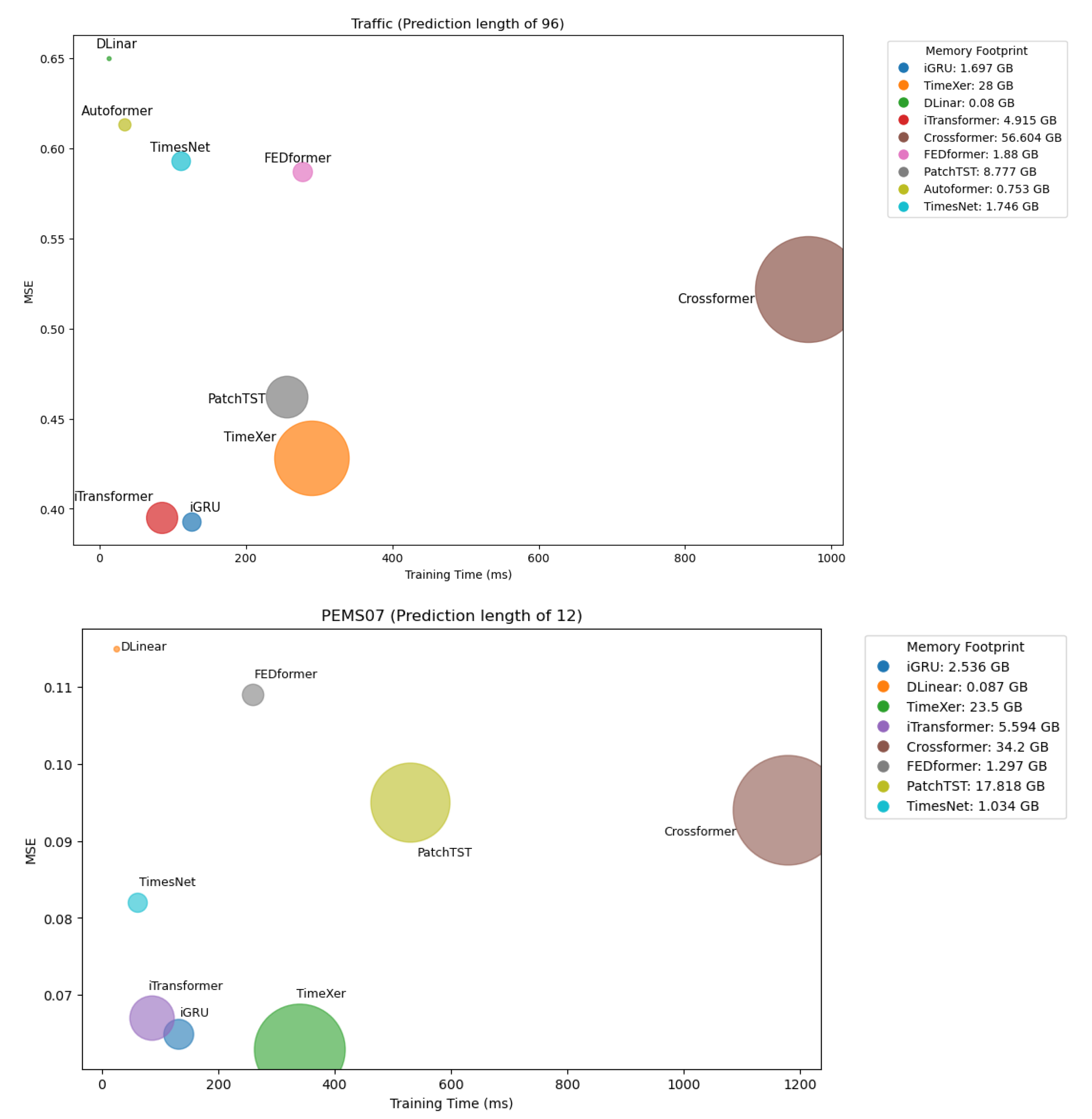
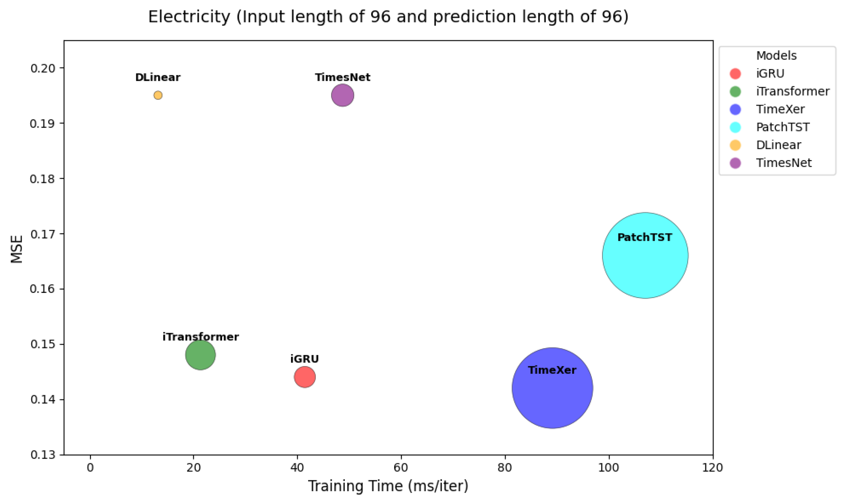
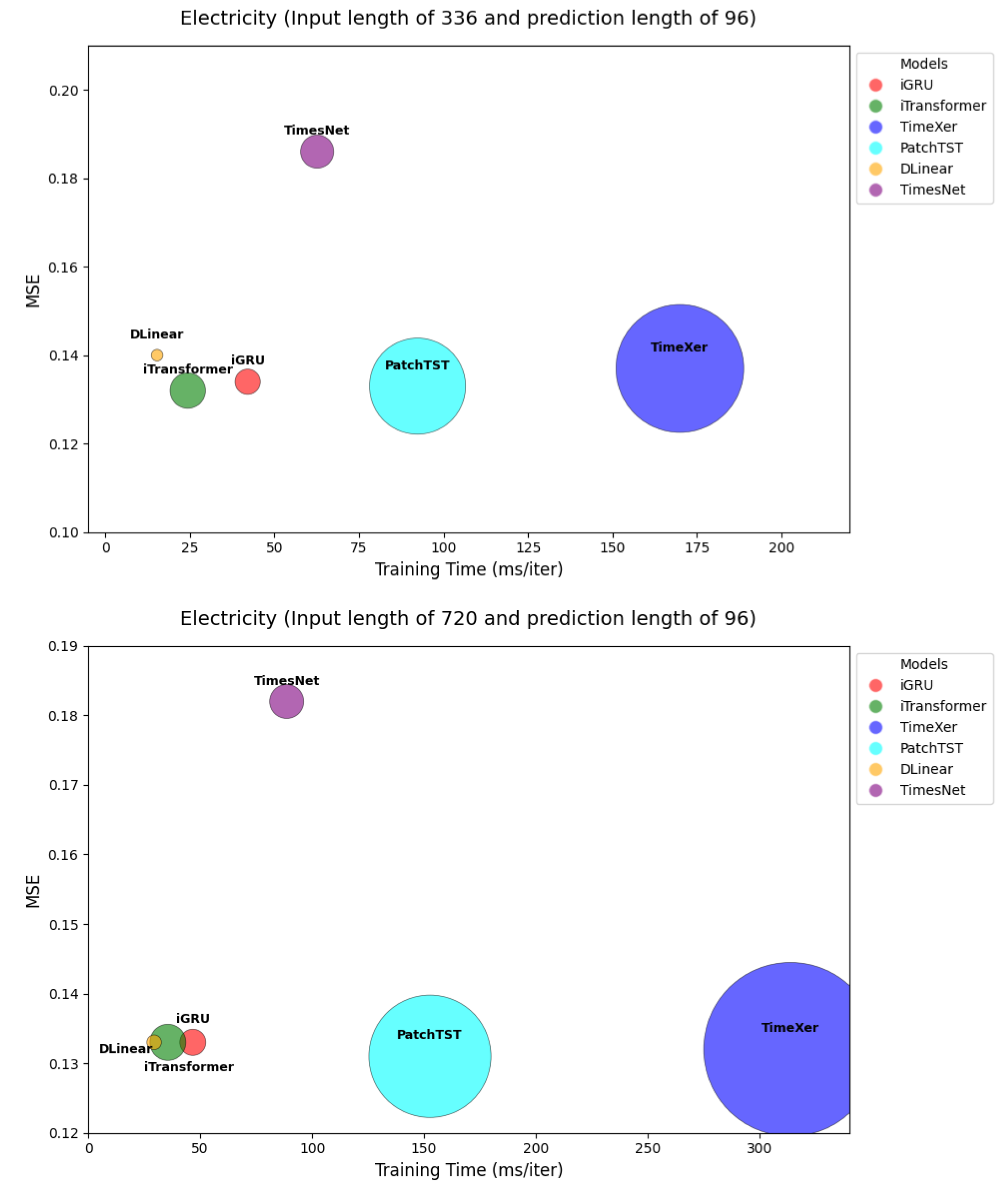
4.1. Model Efficiency

To assess our model’s computational efficiency, its memory consumption and training time are compared against those of the other baselines on the Traffic and PEMS07 datasets. Here, by efficiency, we mean training time and GPU memory consumption. Independent runs are conducted using a single A100-40G GPU with the batch size fixed to 16. Our model’s efficiency is illustrated in Figure 4, where bubble charts show a visual comparison of efficiency metrics. The vertical axis indicates the prediction MSE, and the horizontal axis depicts the duration of one training iteration (milliseconds/iteration). The bubble size indicates the related memory footprint in Gigabytes (total memory consumption in one epoch). As Figure 4 illustrates, the iGRU model attains the most accurate results, while requiring less or equal training time and memory usage compared to other baselines, except the linear models. DLinear consumes minimal memory and time resources than the other models, while delivering the least accurate forecasts. To further support the claim regarding the computational efficiency of iGRU compared to Transformer-based models, we conducted additional experiments on the Electricity dataset with varying input lengths (96, 336, and 720), while keeping the prediction length fixed at 96. For each configuration, we measured the training time (ms/iteration), peak GPU memory usage, and related model performance (MSE). Figure 5 illustrates how model cost varies across different input lengths. Notably, iGRU consistently maintains a short training time and low memory footprint, while delivering competitive or better accuracy compared to Transformer-based alternatives. These results confirm that iGRU offers a stable trade-off between efficiency and performance, specifically when the optimal model is sensitive to the length of input window.

4.2. Ablation Study

We demonstrate the importance of the RNN (GRU) and feed-forward layers in our model through conducting experiments with and without the GRU, feed-forward layer and skip connections. The results are reported in Table 7, showcasing the impact of these components on the iGRU performance. The impact of the above components is mostly evident on the Traffic dataset, which is a complex dataset with many time-series variates. The skip connections added to the outputs of the GRU and feed-forward layers contribute to the gradient flow and training efficiency, which helps to attain optimal results. The significant contribution of GRU blocks in capturing cross-variate correlations becomes evident when comparing the results of the model without GRU blocks (W/O GRU) to those of the iGRU model, which incorporates these blocks. This comparison underscores the potential of GRUs to enhance time-series forecasting performance and prompts a raised discussion on whether RNNs, particularly GRUs, should be reconsidered as a powerful tool in time-series analysis, specifically for modeling cross-channel dependencies.

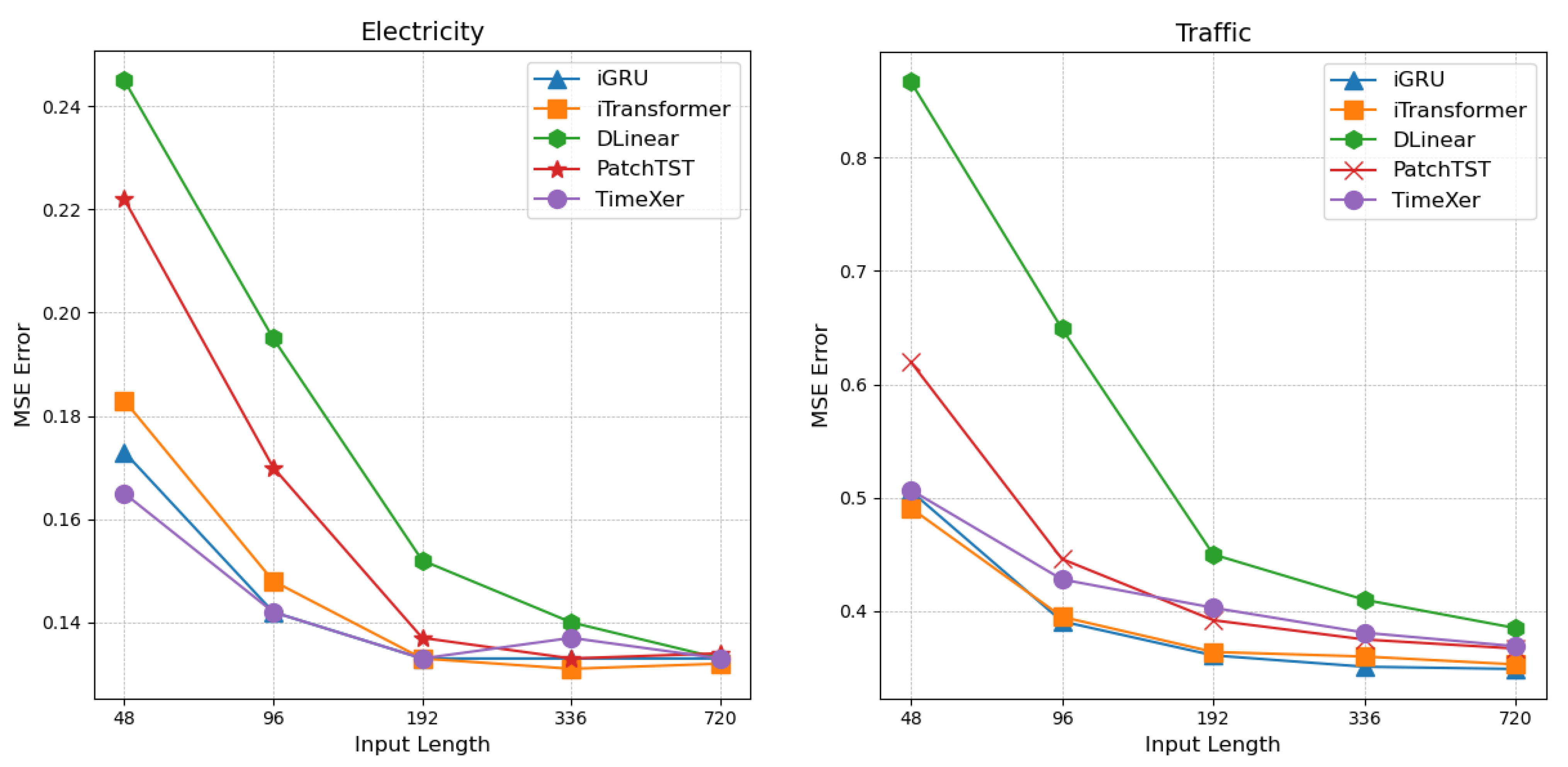
4.3. Increasing Look-Back Length

Some of the previous Transformer-based works [7,19] have shown that increasing the length of look-back window does not necessarily improve the forecasting results, which can be caused by distracted attention on the increasing (prolonged) input. As the structure of our iGRU model is different from the Transformer-based models, we evaluate the performance of iGRU and its main competitor models, e.g., TimeXer, iTransformer, DLinear and PatchTST in Figure 6 using various input lengths. The results pinpoint the performance promotion of iGRU for longer input windows and its capability to leverage the information over the extended temporal context.

5. Conclusions

In this work, recurrent neural network architecture has been brought back to the time-series forecasting field by using it in a different manner and integrating it with a feed-forward layer. Experimentally, the proposed iGRU achieves results that can compete with those of the other state-of-the-art models, while consuming less training time and memory. In future work, we will investigate large-scale foundation models using the iGRU and perform a more in-depth exploration of time-series analysis.

Author Contributions

Conceptualization, V.N. and A.B.D.; methodology, V.N.; software, V.N.; validation, V.N., A.B.D. and M.B.; formal analysis, A.B.D. and V.N.; investigation, V.N., A.B.D. and M.B.; resources, A.B.D. and V.N.; writing—original draft preparation, V.N.; writing—review and editing, V.N., A.B.D. and M.B.; visualization, V.N.; supervision, A.B.D. and M.B.; project administration, A.B.D.; funding acquisition, A.B.D. All authors have read and agreed to the published version of the manuscript.

Funding

This research received no external funding.

Institutional Review Board Statement

Not applicable.

Informed Consent Statement

Not applicable.

Data Availability Statement

The original data presented in the study are openly available at URL: https://drive.google.com/drive/folders/1ZOYpTUa82_jCcxIdTmyr0LXQfvaM9vIy and https://drive.google.com/drive/folders/1Gv1MXjLo5bLGep4bsqDyaNMI2oQC9GH2 (accessed on 22 April 2025).

Conflicts of Interest

The authors declare no conflicts of interest.

References

  1. Chen, Z.; Ma, M.; Li, T.; Wang, H.; Li, C. Long sequence time-series forecasting with deep learning: A survey. Inf. Fusion 2023, 97, 101819. [Google Scholar] [CrossRef]
  2. Challu, C.; Olivares, K.G.; Oreshkin, B.N.; Ramirez, F.G.; Canseco, M.M.; Dubrawski, A. Nhits: Neural hierarchical interpolation for time-series forecasting. In Proceedings of the 37th AAAI Conference on Artificial Intelligence, Washington, DC, USA, 7–14 February 2023; Volume 37, pp. 6989–6997. [Google Scholar]
  3. Chen, S.-A.; Li, C.-L.; Yoder, N.; Arik, S.O.; Pfister, T. Tsmixer: An all-mlp architecture for time-series forecasting. arXiv 2023, arXiv:2303.06053. [Google Scholar]
  4. Zhou, T.; Niu, P.; Sun, L.; Jin, R. One fits all: Power general time-series analysis by pretrained LM. In Proceedings of the 37th International Conference on Neural Information Processing Systems, New Orleans, LA, USA, 10–16 December 2023; Advances in Neural Information Processing Systems 36 (NeurIPS 2023). Neural Information Processing Systems Foundation, Inc. (NeurIPS): San Diego, CA, USA, 2023; pp. 43322–43355. [Google Scholar]
  5. Luo, D.; Wang, X. Moderntcn: A modern pure convolution structure for general time-series analysis. In Proceedings of the Twelfth International Conference on Learning Representations, Vienna, Austria, 7–11 May 2024; pp. 1–43. [Google Scholar]
  6. Liu, M.; Zeng, A.; Xu, Q.; Zhang, L.; Chen, M.; Xu, Q. Scinet: Time-series modeling and forecasting with sample convolution and interaction. In Proceedings of the 36th International Conference on Neural Information Processing Systems, New Orleans, LA, USA, 28 November–9 December 2022; Advances in Neural Information Processing Systems 35 (NeurIPS 2022). Neural Information Processing Systems Foundation, Inc. (NeurIPS): San Diego, CA, USA, 2022; pp. 5816–5828. [Google Scholar]
  7. Zeng, A.; Chen, M.; Zhang, L.; Xu, Q. Are transformers effective for time-series forecasting? In Proceedings of the Thirty-Seventh AAAI Conference on Artificial Intelligence (AAAI-23), Washington, DC, USA, 7–14 February 2023; Volume 37, pp. 11121–11128. [Google Scholar]
  8. Liu, Y.; Hu, T.; Zhang, H.; Wu, H.; Wang, S.; Ma, L.; Long, M. Itransformer: Inverted transformers are effective for time-series forecasting. arXiv 2023, arXiv:2310.06625. [Google Scholar]
  9. Kitaev, N.; Kaiser, L.; Levskaya, A. Reformer: The efficient transformer. In Proceedings of the International Conference on Learning Representations, New Orleans, LA, USA, 6–9 May 2019. [Google Scholar]
  10. Li, Z.; Qi, S.; Li, Y.; Xu, Z. Revisiting long-term time-series forecasting: An investigation on linear mapping. arXiv 2023, arXiv:2305.10721. [Google Scholar]
  11. Lin, S.; Lin, W.; Wu, W.; Zhao, F.; Mo, R.; Zhang, H. Segrnn: Segment recurrent neural network for long-term time-series forecasting. arXiv 2023, arXiv:2308.11200. [Google Scholar]
  12. Hou, B.-J.; Zhou, Z.-H. Learning with interpretable structure from gated RNN. IEEE Trans. Neural Networks Learn. Syst. 2020, 31, 2267–2279. [Google Scholar] [CrossRef] [PubMed]
  13. Elsaraiti, M.; Ali, G.; Musbah, H.; Merabet, A.; Little, T. time-series analysis of electricity consumption forecasting using ARIMA model. In Proceedings of the 2021 IEEE Green Technologies Conference (GreenTech), Denver, CO, USA, 7–9 April 2021; pp. 259–262. [Google Scholar]
  14. Zhou, X.; Chen, W.; Wang, Y.X.; Yan, X. Enhancing the locality and breaking the memory bottleneck of transformer on time-series forecasting. In Proceedings of the 33rd Conference on Neural Information Processing Systems (NeurIPS 2019), Vancouver, BC, Canada, 8–14 December 2019; Advances in Neural Information Processing Systems 32 (NeurIPS 2019). Neural Information Processing Systems Foundation, Inc. (NeurIPS): San Diego, CA, USA, 2019. [Google Scholar]
  15. Zhou, H.; Zhang, S.; Peng, J.; Zhang, S.; Li, J.; Xiong, H.; Zhang, W. Informer: Beyond efficient transformer for long sequence time-series forecasting. In Proceedings of the Thirty-Fifth AAAI Conference on Artificial Intelligence (AAAI-21), Virtually, 2–9 February 2021; Volume 35, pp. 11106–11115. [Google Scholar]
  16. Wu, H.; Xu, J.; Wang, J.; Long, M. Autoformer: Decomposition transformers with auto-correlation for long-term series forecasting. In Proceedings of the 35th Conference on Neural Information Processing Systems (NeurIPS 2021), Online, 6–14 December 2021; Advances in Neural Information Processing Systems 34 (NeurIPS 2021). Neural Information Processing Systems Foundation, Inc. (NeurIPS): San Diego, CA, USA, 2021; pp. 22419–22430. [Google Scholar]
  17. Zhou, T.; Ma, Z.; Wen, Q.; Wang, X.; Sun, L.; Jin, R. Fedformer: Frequency enhanced decomposed transformer for long-term series forecasting. In Proceedings of the 39th International Conference on Machine Learning PMLR 2022, Baltimore, MD, USA, 17–23 July 2022; pp. 27268–27286. [Google Scholar]
  18. Liu, S.; Yu, H.; Liao, C.; Li, J.; Lin, W.; Liu, A.X.; Dustdar, S. Pyraformer: Low-complexity pyramidal attention for long-range time-series modeling and forecasting. In Proceedings of the Tenth International Conference on Learning Representations (ICLR 2022), Virtual, 25–29 April 2022. [Google Scholar]
  19. Nie, Y.; Nguyen, N.H.; Sinthong, P.; Kalagnanam, J. A time-series is worth 64 words: Long-term forecasting with transformers. arXiv 2022, arXiv:2211.14730. [Google Scholar]
  20. Zhang, Y.; Yan, J. Crossformer: Transformer utilizing cross-dimension dependency for multivariate time-series forecasting. In Proceedings of the Eleventh International Conference on Learning Representations, Kigali, Rwanda, 1–5 May 2023. [Google Scholar]
  21. Das, A.; Kong, W.; Leach, A.; Mathur, S.; Sen, R.; Yu, R. Long-term forecasting with tide: Time-series dense encoder. arXiv 2023, arXiv:2304.08424. [Google Scholar]
  22. Wu, H.; Hu, T.; Liu, Y.; Zhou, H.; Wang, J.; Long, M. Timesnet: Temporal 2d-variation modeling for general time-series analysis. arXiv 2022, arXiv:2210.02186. [Google Scholar]
  23. Wang, Y.; Zhang, L.; Chen, M.; Xu, Q.; Zeng, A. Timexer: Empowering transformers for time-series forecasting with exogenous variables. In Proceedings of the Thirty-Eighth Annual Conference on Neural Information Processing Systems, Vancouver, BC, Canada, 9–15 December 2024; Advances in Neural Information Processing Systems 37 (NeurIPS 2024). Neural Information Processing Systems Foundation, Inc. (NeurIPS): San Diego, CA, USA, 2024. [Google Scholar]
  24. Cho, K.; van Merriënboer, B.; Gulcehre, C.; Bahdanau, D.; Bougares, F.; Schwenk, H.; Bengio, Y. Learning phrase representations using RNN encoder-decoder for statistical machine translation. arXiv 2014, arXiv:1406.1078. [Google Scholar]
  25. Wang, C.; Liu, Z.; Wei, H.; Chen, L.; Zhang, H. Hybrid deep learning model for short-term wind speed forecasting based on time-series decomposition and gated recurrent unit. Complex Syst. Model. Simul. 2021, 1, 308–321. [Google Scholar] [CrossRef]
  26. Lawi, A.; Mesra, H.; Amir, S. Implementation of long short-term memory and gated recurrent units on grouped time-series data to predict stock prices accurately. J. Big Data 2022, 9, 89. [Google Scholar] [CrossRef]
  27. Kim, T.; Kim, J.; Tae, Y.; Park, C.; Choi, J.-H.; Choo, J. Reversible instance normalization for accurate time-series forecasting against distribution shift. In Proceedings of the International Conference on Learning Representations, Vienna, Austria, 4 May 2021. [Google Scholar]
  28. Chen, C.; Petty, K.; Skabardonis, A.; Varaiya, P.; Jia, Z. Freeway performance measurement system: Mining loop detector data. Transp. Res. Rec. 2001, 1748, 96–102. [Google Scholar] [CrossRef]
  29. Paszke, A.; Gross, S.; Massa, F.; Lerer, A.; Bradbury, J.; Chanan, G.; Killeen, T.; Lin, Z.; Gimelshein, N.; Antiga, L.; et al. Pytorch: An imperative style, high-performance deep learning library. In Proceedings of the 33rd International Conference on Neural Information Processing Systems, Vancouver, BC, Canada, 8–14 December 2019; Advances in Neural Information Processing Systems 32 (NeurIPS 2019). Neural Information Processing Systems Foundation, Inc. (NeurIPS): San Diego, CA, USA, 2019. [Google Scholar]
  30. Kingma, D.P.; Ba, J. Adam: A method for stochastic optimization. arXiv 2014, arXiv:1412.6980. [Google Scholar]
Figure 1. An example of a multivariate time-series which consists of multiple channels (variates). There are inter-variate dependencies between the channels and temporal correlations between different time-steps.
Ai 06 00090 g001
Figure 2. Illustration of iGRU architecture.
Ai 06 00090 g002
Figure 3. Visual comparison of iGRU and iTransformer on different datasets. The orange line indicates predictions for iGRU and green line corresponds to predictions for iTransformer, with the blue line indicating the ground truth. The look-back window and forecast window lengths are set to 96 for all datasets.
Ai 06 00090 g003
Figure 4. Comparison of iGRU with other baselines in terms of MSE, training time and GPU memory usage on Traffic and PEMS07 datasets. The look-back window is set to 96 and the prediction length is set to 96 and 12 for the Traffic and PEMS07 datasets, respectively.
Ai 06 00090 g004
Figure 5. Comparison of training time (ms/iter), model performance (MSE), and memory usage (bubble size) across different input lengths on the Electricity dataset. iGRU consistently demonstrates a low training cost and memory usage while maintaining competitive or better performance compared to Transformer-based models.
Ai 06 00090 g005aAi 06 00090 g005b
Figure 6. Forecasting with look-back length in {48, 96, 192, 336, 720} and prediction length of 96 on the Electricity and Traffic datasets. The proposed iGRU model exploits enlarged and shortened input lengths and delivers accurate results.
Ai 06 00090 g006
Table 1. Comparison of time and memory complexity for different models, where L represents the input sequence length (context length).
MethodTypeTime ComplexityMemory Complexity
GRURNN O ( L ) O ( L )
DLinearMLP O ( L ) O ( L )
CrossformerTransformer O ( L 2 ) O ( L 2 )
Table 2. Dataset information: Dim represents the number of variates and Dataset Size denotes the total number of time points in (Training, Validation, Testing) split of each dataset, respectively. Prediction Length indicates the future time points to be predicted and four prediction lengths settings are specified in each dataset. Frequency denotes the sampling interval of time points.
DatasetDimPrediction LengthDataset SizeFrequencyInformation
ETTm1, ETTm27{96, 192, 336, 720}(34,465, 11,521, 11,521)15 minElectricity
Exchange8{96, 192, 336, 720}(5120, 665, 1422)DailyEconomy
Weather21{96, 192, 336, 720}(36,792, 5271, 10,540)10 minWeather
Electricity321{96, 192, 336, 720}(18,317, 2633, 5261)HourlyElectricity
Traffic862{96, 192, 336, 720}(12,185, 1757, 3509)HourlyTransportation
Solar-Energy137{96, 192, 336, 720}(36,601, 5161, 10,417)10 minEnergy
PEMS03358{12, 24, 48, 96}(15,617, 5135, 5135)5 minTransportation
PEMS04307{12, 24, 48, 96}(10,172, 3375, 3375)5 minTransportation
PEMS07883{12, 24, 48, 96}(16,911, 5622, 5622)5 minTransportation
PEMS08170{12, 24, 48, 96}(10,690, 3548, 3548)5 minTransportation
Table 3. Selected hyper-parameters for training the iGRU model on different benchmarks.
DatasetModel DimensionFeed-Forward DimensioniGRU BlocksLearning RateBatch SizeDropout
ETTm125651220.0001320.1
ETTm225651220.0001320.1
Weather51251230.0001320.1
Exchange25625620.00005320.1
Electricity51251230.001160.1
Traffic51251240.001160.1
PEMS0351251240.001160.1
PEMS041024102440.001160.1
PEMS075125123 or 40.001160.1
PEMS085125123 or 40.001160.1
Table 4. Multivariate time-series forecasting results of iGRU and the baseline models on Traffic and PEMS datasets. The input length (lookback window) is set to 96 and the prediction length is in {12, 24, 48, 96} for PEMS datasets and in {96, 192, 336, 720} for Traffic dataset. The best results are shown in bold, and the second-best results are shown in italics.
ModelsOursTimeXeriTransformerPatchTSTDLinearCrossformerTimesNetTiDEFEDformerAutoformer
MetricMSEMAEMSEMAEMSEMAEMSEMAEMSEMAEMSEMAEMSEMAEMSEMAEMSEMAEMSEMAE
960.3930.2680.4280.2710.3950.2680.4620.2950.6500.3960.5220.2900.5930.3210.8050.4930.5870.3660.6130.388
1920.4170.2770.4480.2820.4170.2760.4660.2960.5980.3700.5300.2930.6170.3360.7560.4740.6040.3730.6160.382
Traffic3360.4310.2830.4730.2890.4330.2830.4820.3040.6050.3730.5580.3050.6290.3360.7620.4770.6210.3830.6220.337
7200.4630.3010.5160.3070.4670.3020.5140.3220.6450.3940.5890.2380.6400.3500.7190.4490.6260.3820.6600.408
Avg0.4260.2820.4660.2870.4280.2820.4810.3040.6250.3830.5500.3040.6200.3360.7600.4730.6100.3760.6280.379
120.0690.1720.0720.1840.0710.1740.0990.2160.1220.2430.0900.2030.0850.1920.1780.3050.1260.2510.2720.385
240.0870.1950.0880.2020.0930.2010.1420.2590.2010.3170.1210.2400.1180.2230.2570.3710.1490.2750.3340.440
PEMS03480.1190.2300.1270.2420.1250.2360.2110.3190.3330.4250.2020.3170.1550.2600.3790.4630.2270.3481.0320.782
960.1510.2640.1770.2840.1640.2750.2690.3700.4570.5150.2620.3670.2280.3170.4900.5390.3480.4341.0310.796
Avg0.1070.2150.1160.2280.1130.2210.1800.2910.2780.3750.1690.2810.1470.2480.3260.4190.2130.3270.6670.601
120.0780.1850.0820.1970.0780.1830.1050.2240.1480.2720.0980.2180.0870.1950.2190.3400.1380.2620.4240.491
240.0910.2040.0940.2120.0950.2050.1530.2750.2240.3400.1310.2560.1030.2150.2920.3980.1770.2930.4590.509
PEMS04480.1140.2300.1190.2370.1200.2330.2290.3390.3550.4370.2050.3260.1360.2500.4090.4780.2700.3680.6460.610
960.1410.2540.1620.2750.1500.2620.2910.3890.4520.5040.4020.4570.1900.3030.4920.5320.3410.4270.9120.748
Avg0.1060.2180.1140.2300.1110.2210.1950.3070.2950.3880.2090.3140.1290.2410.3530.4370.2310.3370.6100.590
120.0650.1630.0630.1710.0670.1650.0950.2070.1150.2420.0940.2000.0820.1810.1730.3040.1090.2250.1990.336
240.0840.1880.0790.1870.0880.1900.1500.2620.2100.3290.1390.2470.1010.2040.2710.3830.1250.2440.3230.420
PEMS07480.1030.2100.1000.2030.1100.2150.2530.3400.3980.4580.3110.3690.1340.2380.4460.4950.1650.2880.3900.470
960.1280.2350.1310.2330.1390.2450.3460.4040.5940.5530.3960.4420.1810.2790.6280.5770.2620.3760.5540.578
Avg0.0950.1990.0930.1990.1010.2040.2110.3030.3290.3950.2350.3150.1930.2710.3800.4400.1650.2830.3670.451
120.0770.1790.0910.2060.0790.1820.1680.2320.1540.2760.1650.2140.1120.2120.2270.3430.1730.2730.4360.485
240.1090.2120.1330.2530.1150.2190.2240.2810.2480.3530.2150.2600.1410.2380.3180.4090.2100.3010.4670.502
PEMS08480.1770.2320.2090.2490.1860.2350.3210.3540.4400.4700.3150.3550.1980.2830.4970.5100.3200.3940.9660.733
960.2130.2620.4920.4670.2210.2670.4080.4170.6740.5650.3770.3970.3200.3510.7210.5920.4420.4651.3850.915
Avg0.1440.2210.2310.2940.1500.2260.2800.3210.3790.4160.2680.3070.1930.2710.4410.4640.2860.3580.8140.659
Table 5. Multivariate time-series forecasting results of iGRU and the baseline models on Weather, Electricity, Exchange, Solar-energy, ETTm1 and ETTm2 datasets. The input length (look-back window) is set to 96 and the prediction length is {96, 192, 336, 720}. The best results are shown in bold, and the second-best results are shown in italics.
ModelsOursTimeXeriTransformerPatchTSTDLinearCrossformerTimesNetTiDEFEDformerAutoformer
MetricMSEMAEMSEMAEMSEMAEMSEMAEMSEMAEMSEMAEMSEMAEMSEMAEMSEMAEMSEMAE
960.1670.2100.1570.2050.1740.2140.1770.2180.1960.2550.1580.2300.1720.2200.2020.2610.2170.2960.2660.336
1920.2150.2540.2040.2470.2210.2540.2250.2590.2370.2960.2060.2770.2190.2610.2420.2980.2760.3360.3070.367
Weather3360.2730.2970.2610.2900.2780.2960.2780.2970.2830.3350.2720.3350.2800.3060.2870.3350.3390.3800.3590.395
7200.3540.3490.3400.3410.3580.3470.3540.3480.3450.3810.3980.4180.3650.3590.3510.3860.4030.4280.4190.428
Avg0.2530.2780.2410.2710.2580.2780.2590.2810.2650.3170.2590.3150.2590.2870.2710.3200.3090.3600.3380.382
960.1420.2380.1400.2420.1480.2400.1810.2700.1970.2820.2190.3140.1680.2720.2370.3290.1930.3080.2010.317
1920.1600.2550.1570.2560.1620.2530.1880.2740.1960.2850.2310.3220.1840.2890.2360.3300.2010.3150.2220.334
Electricity3360.1760.2720.1760.2750.1780.2690.2040.2930.2090.3010.2460.3370.1980.3000.2490.3440.2140.3290.2310.338
7200.2100.3010.2110.3060.2250.3170.2460.3240.2450.3330.2800.3630.2200.3200.2840.3730.2460.3550.2540.361
Avg0.1720.2670.1710.2700.1780.2700.2050.2900.2120.3000.2440.3340.1920.2950.2510.3440.2140.3270.2270.338
960.1940.2430.1870.2500.2030.2370.2340.2860.2900.3780.3100.3310.2500.2920.3120.3990.2420.3420.8840.711
1920.2080.2550.2020.2710.2330.2610.2670.3100.3200.3980.7340.7250.2960.3180.3390.4160.2850.3800.8340.692
Solar3360.2140.2710.2150.2840.2480.2730.2900.3150.3530.4150.7500.7350.3190.3300.3680.4300.2820.3760.9410.723
7200.2140.2640.2200.2930.2490.2750.2890.3170.3560.4130.7690.7650.3380.3370.3700.4250.3570.4270.8820.717
Avg0.2080.2580.2290.2740.2330.2620.2700.3070.3300.4010.6410.6390.3010.3190.3470.4170.2910.3810.8850.711
960.0860.2070.0860.2060.0860.2060.0880.2050.0880.2180.2560.3670.1070.2340.0940.2180.1480.2780.1970.323
1920.1810.3040.1880.3080.1770.2990.1760.2990.1760.3150.4700.5090.2260.3440.1840.3070.2710.3150.3000.369
Exchange3360.3310.4170.3420.4210.3310.4170.3010.3970.3130.4271.2680.8830.3670.4480.3490.4310.4600.4270.5090.524
7200.8570.7020.8700.7020.8470.6910.9010.7140.8390.6951.7671.0680.9640.7460.8520.6981.1950.6951.4470.941
Avg0.3640.4080.3720.4090.3600.4030.3670.4040.3540.4140.9400.7070.4160.4430.3700.4130.5190.4290.6130.539
960.3210.3580.3180.3560.3340.3680.3290.3670.3450.3720.4040.4260.3380.3750.3640.3870.3790.4190.5050.475
1920.3640.3820.3620.3830.3770.3910.3670.3850.3800.3890.4500.4510.3740.3870.3980.4040.4260.4410.5530.496
ETTm13360.3990.4060.3950.4070.4260.4200.3990.4100.4130.4130.5320.5150.4100.4110.4280.4250.4450.4590.6210.537
7200.4700.4450.4520.4410.4910.4590.4540.4390.4740.4530.6660.5890.4780.4504870.4610.5430.4900.6710.561
Avg0.3890.3980.3820.3970.4070.4100.3870.4000.4030.4070.5130.4960.4000.4060.4190.4190.4480.4520.5880.517
960.1770.2600.1710.2560.1800.2640.1750.2590.1930.2920.2870.3660.1870.2670.2070.3050.2030.2870.2550.339
1920.2420.3040.2370.2990.2500.3090.2410.3020.2840.3620.4140.4920.2490.3040.2900.3640.2690.3280.2810.340
ETTm23360.3060.3430.2960.3380.3110.3480.3050.3430.3690.4270.5970.5420.3210.3510.3770.4220.3250.3660.3390.372
7200.4080.4060.3920.3940.4120.4070.4020.4120.5540.5221.7301.0420.4080.4030.5580.5240.4210.4150.4330.432
Avg0.2830.3280.2740.3220.2880.3320.2810.3260.3500.4010.7570.6100.2900.3330.3580.4040.3050.3490.3270.371
Table 6. Robustness of iGRU model. Five independent runs are conducted with different random seeds.
DatasetElectricityTrafficWeather
HorizonMSEMAEMSEMAEMSEMAE
960.142 ± 0.0000.238 ± 0.0000.393 ± 0.0010.267 ± 0.0010.167 ± 0.0020.210 ± 0.001
1920.160 ± 0.0000.254 ± 0.0000.416 ± 0.0000.277 ± 0.0010.215 ± 0.0000.254 ± 0.001
3360.176 ± 0.0000.272 ± 0.0000.431 ± 0.0000.283 ± 0.0000.273 ± 0.0000.297 ± 0.000
7200.210 ± 0.0030.301 ± 0.0030.463 ± 0.0000.301 ± 0.0000.354 ± 0.0010.349 ± 0.001
DatasetETTm1ETTm2Exchange
HorizonMSEMAEMSEMAEMSEMAE
960.320 ± 0.0010.358 ± 0.0010.178 ± 0.0000.260 ± 0.0000.086 ± 0.0000.207 ± 0.000
1920.364 ± 0.0000.382 ± 0.0000.244 ± 0.0010.304 ± 0.0010.181 ± 0.0000.304 ± 0.000
3360.398 ± 0.0000.405 ± 0.0000.304 ± 0.0010.343 ± 0.0000.331 ± 0.0000.417 ± 0.000
7200.469 ± 0.0010.445 ± 0.0000.408 ± 0.0010.403 ± 0.0010.857 ± 0.0000.702 ± 0.000
Table 7. Ablation of iGRU model without GRU, skip or residual connections and feed-forward layer. The best results are shown in bold.
DesignW/O
F.F
W/O F.F
+
W/O Skip
Connection
W/O Skip
Connection
W/O GRUiGRU
MetricMSEMAEMSEMAEMSEMAEMSEMAEMSEMAE
960.3240.3610.3250.3640.3270.3640.3240.3620.3210.358
ETTm11920.3660.3830.3680.3870.3730.3900.3670.3840.3640.382
3360.3990.4050.4030.4100.4150.4180.4000.4060.3990.406
7200.4670.4430.4750.4500.4820.4550.4670.4440.4700.445
960.4070.2810.4140.2870.5020.3660.4370.2820.3930.268
Traffic1920.4280.2890.4370.2960.5350.3720.4500.2870.4170.277
3360.4450.2960.4520.3030.5370.3710.4640.2940.4310.283
7200.4760.3130.4870.3230.5720.3890.4950.3120.4630.301
960.1700.2140.1660.2110.1690.2130.1940.2320.1680.211
Weather1920.2170.2560.2140.2550.2170.2570.2390.2690.2150.254
3360.2740.2970.2710.2960.2770.3000.2910.3070.2740.297
7200.3530.3490.3530.3490.3570.3520.3640.3540.3540.348
Disclaimer/Publisher’s Note: The statements, opinions and data contained in all publications are solely those of the individual author(s) and contributor(s) and not of MDPI and/or the editor(s). MDPI and/or the editor(s) disclaim responsibility for any injury to people or property resulting from any ideas, methods, instructions or products referred to in the content.

