Non-Linear Synthetic Time Series Generation for Electroencephalogram Data Using Long Short-Term Memory Models

Abstract

Background/Objectives: The implementation of artificial intelligence-based systems for disease detection using biomedical signals is challenging due to the limited availability of training data. This paper deals with the generation of synthetic EEG signals using deep learning-based models, to be used in future research for training Parkinson’s disease detection systems. Methods: Linear models, such as AR, MA, and ARMA, are often inadequate due to the inherent non-linearity of time series. To overcome this drawback, long short-term memory (LSTM) networks are proposed to learn long-term dependencies in non-linear EEG time series and subsequently generate synthetic signals to enhance the training of detection systems. To learn the forward and backward time dependencies in the EEG signals, a Bidirectional LSTM model has been implemented. The LSTM model was trained on the UC San Diego Resting State EEG Dataset, which includes samples from two groups: individuals with Parkinson’s disease and a healthy control group. Results: To determine the optimal number of cells in the model, we evaluated the mean squared error (MSE) and cross-correlation between the original and synthetic signals. This method was also applied to select the length of the hidden state vector. The number of hidden cells was set to 14, and the length of the hidden state vector for each cell was fixed at 4. Increasing these values did not improve MSE or cross-correlation and unnecessarily increased computational complexity. The proposed model’s performance was evaluated using the mean-squared error (MSE), Pearson’s correlation coefficient, and the power spectra of the synthetic and original signals, demonstrating the suitability of the proposed method for this application. Conclusions: The proposed model was compared to Autoregressive Moving Average (ARMA) models, demonstrating superior performance. This confirms that deep learning-based models, such as LSTM, are strong alternatives to statistical models like ARMA for handling non-linear, multifrequency, and non-stationary signals.

1. Introduction

This paper deals with a problem that arises in the application of machine learning (ML) models for Parkinson’s disease (PD) detection using electroencephalogram (EEG) signals. PD is a neurological disorder that affects movement, causing tremors, fatigue, muscle stiffness, and difficulty walking [1]. Biomedical data from patients with PD are scarce, primarily because the affected individuals are typically older, and it is not easy for them to cooperate in undergoing the necessary tests to generate large databases [2].

However, the performance of ML models heavily depends on data quality and availability [3]. A considerable amount of clean, representative, and non-sparse data is required, but gathering sufficient data to train and test reliable models may be challenging, costly, or unfeasible. For this reason, the application of data augmentation techniques has emerged as an alternative to scarcity.

Therefore, the primary motivation of this research is to generate synthetic EEG signals from PD patients with the goal of using them in the near future to train systems for disease detection. EEG-based diagnosis is not only more affordable than imaging-based methods but also has the potential for widespread adoption in developing countries. Furthermore, the approach proposed in this paper can be extended to other medical challenges where the lack of adequate datasets limits the application of artificial intelligence techniques. Several diagnostic fields that rely on biosignals could benefit from this methodology, including:

• Electrocardiogram (ECG) analysis for detecting heart disorders.
• EEG analysis for assessing brain electrical activity.
• Electromyography (EMG) analysis for evaluating muscle signal activity.

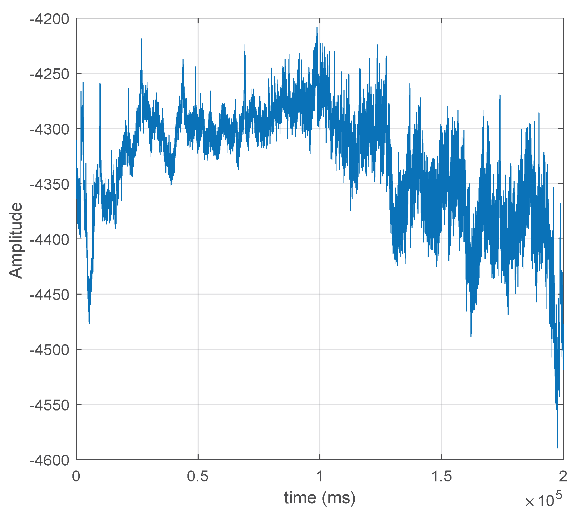
EEG signals are electrical signals generated by the brain’s neuronal activity and recorded from the scalp. They reflect the collective electrical activity of neurons, primarily in the cerebral cortex. EEG signals can be used to measure and monitor brain function [4] and have recently been proposed as source of information for early detection of PD [5,6,7]. EEG signals are examples of time series data that are collected and organized in chronological order [8]. An example of an EEG signal is shown in Figure 1, illustrating its random nature, which makes prediction difficult.

Time series data processing is a major challenge in data science, especially when the series are long, complex, and non-linear. Discovering hidden patterns in these series requires advanced techniques that combine statistical models and artificial intelligence algorithms [9]. The philosophy of time series forecasting lies in the ability to estimate future values based on previous observations. Despite the importance of these forecasts, their implementation presents many challenges. Noise and missing values often degrade time series data quality, negatively impacting forecast accuracy. Additionally, using inappropriate forecasting models or insufficient data can further reduce their effectiveness [10].

Time series can also be processed for classification purposes. In this study, we aim to classify EEG time series based on the characteristics of the individuals who produced them. Specifically, we aim to perform binary classification to determine whether a person has PD. Classifiers based on artificial intelligence techniques or statistical methods, especially deep learning-based models, require large amounts of data for training and testing. When sufficient data are unavailable, generating synthetic data has been suggested, as this has been shown to improve training.

Currently, various methods exist for generating synthetic data, which can be classified into two main types: traditional methods and machine learning-based techniques. Traditional methods include models such as autoregressive (AR), moving average (MA), autoregressive moving average (ARMA) [11], and autoregressive integrated moving average (ARIMA) [12]. While effective, these models have certain limitations. Traditional methods require smooth and stationary data, which are not always available in real-world scenarios where time series data are often turbulent and unstable [13]. With the rapid advancement of AI technology, researchers have shifted their focus toward neural networks and deep learning techniques to overcome the challenges of traditional models [14].

One effective tool for this purpose is long short-term memory (LSTM) [15], a type of recurrent neural network (RNN) capable of handling complex temporal data. LSTM is a powerful tool for time series analysis due to its ability to retain information across long sequences of data. It is widely used in applications that require understanding non-linear and complex temporal patterns, such as analyzing financial and medical data and generating synthetic data that resemble the original data [16].

In this paper, we use long short-term memory (LSTM) networks to model the generation of EEG time series data, highlighting their effectiveness in capturing the complex temporal dependencies inherent in neural signals. The ability of LSTM to retain and utilize long-term patterns makes it particularly suitable for handling the dynamic and non-linear properties of EEG data. LSTM-based models can effectively reproduce the complex behavior of EEG time series, offering promising potential for synthetic data generation and other applications in neurophysiological research.

This study opens the door to further experiments by using the augmented dataset to train classification models with the generated data and validating them using the original data. This research direction can be explored in future work, though it is not addressed in this paper. Several methods have been proposed in the literature to expand the dataset, commonly referred to as “data augmentation techniques”. These include signal reflections, noise addition, and more. Models capable of generating EEG signals from real data enable the application of innovative techniques and strategies, which will be explored in future studies. For example, the generated model for one patient could be used to predict data for a different patient. This method would produce a prediction that retains the general characteristics of an EEG signal but differs from both real signals. The prediction error could then be interpreted as the difference that makes the signal unique. In this way, the dataset size could grow multiplicatively, helping to mitigate overfitting issues caused by small training sets.

Our approach focuses on time series prediction and is not designed for generating synthetic images. Alternative methods in the literature employ deep learning architectures, such as generative adversarial networks (GANs) and diffusion models, which are better suited for image generation.

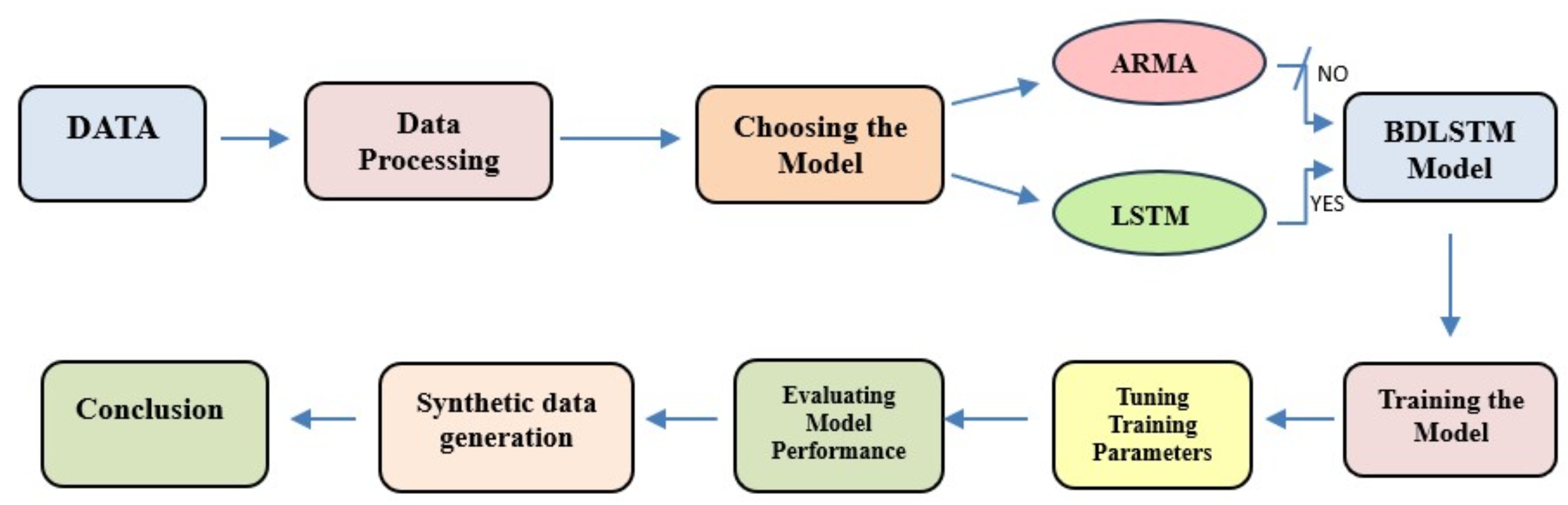
The research presented in this paper follows a structured workflow consisting of several key steps. First, the available data were pre-processed to reduce noise and normalize signal amplitudes. Next, the model for generating synthetic signals was selected. A comparison was made between statistical models—specifically, ARMA models—and LSTM-based models, with the latter demonstrating superior performance. Ultimately, bidirectional LSTM (BD-LSTM) was chosen to leverage both forward and backward information. The model’s parameters, including the number of hidden cells and the size of the hidden state vector, were fine-tuned to achieve optimal results. Finally, the model’s performance was evaluated using both quantitative quality metrics and visual comparison between synthetic and real signals. The overall research workflow is illustrated in Figure 2.

This paper is organized as follows: Section 1 introduces the problem addressed. Section 2 reviews related works and key concepts of LSTM models and their application in generating synthetic signals. Section 3 describes the materials and methods used in this research. The results are presented and discussed in Section 4. Finally, Section 5 provides the conclusions.

2. Review of Knowledge and Related Works

This study investigates the use of electroencephalography (EEG) data to train machine learning models for diagnosing PD. The scarcity of data suitable for effective training has led to the generation of synthetic datasets. An example of this approach is presented in [16], where generative adversarial networks (GANs) were employed. The synthetic data generated were subsequently used to retrain convolutional neural network (CNN)-based detectors, and the performance of these models was compared to that of baseline detectors.

The creation of synthetic data is also referred to as “data augmentation”. In [17], various data augmentation techniques were systematically compared. The study evaluated 13 different methods for generating synthetic data across two tasks: sleep stage classification and motor imagery classification within the context of brain–computer interfaces (BCIs). These methods involved applying various transformations to EEG signals in the temporal, frequency, and spatial domains. Two distinct EEG datasets were utilized for these tasks, each with corresponding predictive models. The findings indicated that employing appropriate data augmentation techniques could enhance classification accuracy by up to 45% compared to models trained without augmentation. The experiments were conducted using the open-source Python library “scikit-learn” for data generation and testing.

A significant challenge in generating synthetic EEG data is the non-stationarity of EEG signals, which complicates the application of linear prediction methods. To address this issue, ref. [18] transformed short-time magnetoencephalography (MEG) signals to the frequency domain. For dominant frequencies in the 8–12 Hz range, time-series representations were derived, and their stationarity and Gaussianity were assessed. Autoregressive moving average (ARMA) models were then proposed to describe these stationary time series.

Long short-term memory (LSTM) has been utilized to model the volatile and non-linear behaviors characteristics of EEG signals. Similar signal dynamics are observed in the stock market. In [19], single-layer and multi-layer LSTM models were developed to predict stock market trends. These models were compared using metrics such as root mean square error (RMSE), mean absolute percentage error (MAPE), and the correlation coefficient (R), revealing that single-layer LSTM model provides a better fit and higher prediction accuracy.

LSTM networks have also been applied to long-term energy consumption forecasting to capture data periodicity. The proposed strategy outperformed traditional forecasting techniques by reducing RMSE by 54.85%, 64.59%, and 19.7%, respectively. Additionally, the study indicated that the algorithm exhibited strong generalization capabilities, even with fewer secondary variables [20].

2.1. LSTM Model

A neural network with a long short-term memory (LSTM) hidden layer is a type of recurrent neural network (RNN) that is primarily used to process sequential data such as text, time series, or audio sequences. LSTM is designed to address the problem of long-term dependencies, a significant limitation of traditional RNNs [21].

LSTM has a specialized architecture that enables it to retain and propagate information over long sequences, thereby preventing the learning process from being hindered by the vanishing gradient problem [22]. When a neural network has an LSTM hidden layer, its operation follows these key steps:

• The input to the network is sequential, meaning the model receives a sequence of vectors, one per time step. The sequence of inputs is fed into the model one step at a time.
• Instead of using a simple dense layer like traditional neural networks, LSTM networks utilize LSTM cells in the hidden layer, specifically designed to store and process information efficiently over time.
• After passing through the LSTM layer, the output ${\mathbf{h}}_t$ can serve various purposes, depending on the task. In a classification or regression model (e.g., time series prediction), the last hidden state ${\mathbf{h}}_t$ can be passed to a final dense layer to produce the output.

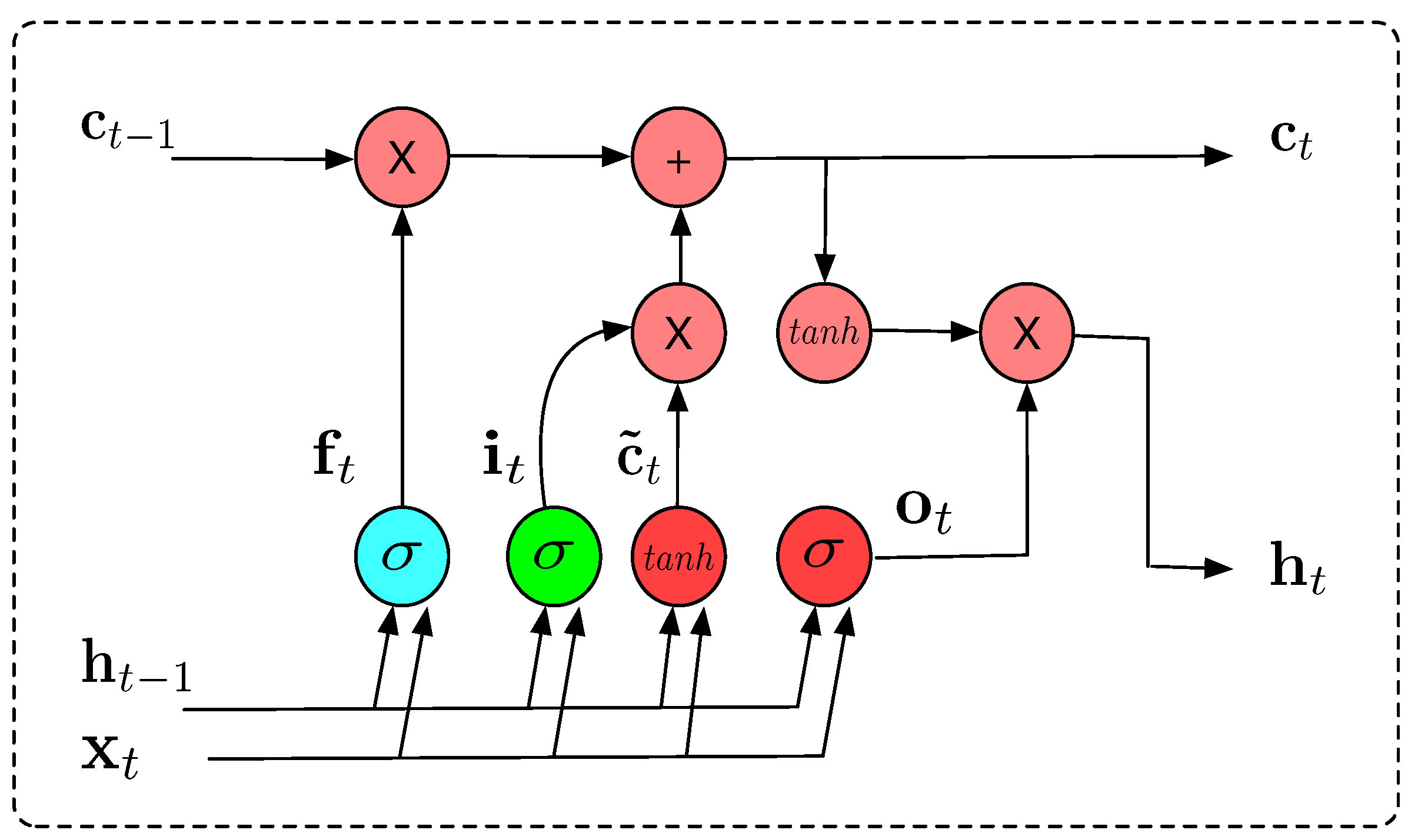
The architecture of the LSTM hidden layer is composed of a series of repeating blocks or cells, which process the information in the input vector, the hidden state, and the cell state. The information processed by the LSTM cell is as follows:

1.

Input vector at each time step, ${\mathbf{x}}_t$.

2.

Hidden state vector, ${\mathbf{h}}_t$, which represents the current memory of the network. It is initialized to a vector of zeros.

3.

Cell state vector ${\mathbf{c}}_t$ with information from the previous cell. It is responsible for storing long-term information over the course of the sequence.

The flow of information through the cell is controlled with three types of gates:

• Forget gate, which processes the previous hidden vector ${\mathbf{h}}_{t-1}$ and the current input ${\mathbf{x}}_t$ to produce an output between 0 and 1:

  $${\mathbf{f}}_t=\sigma ({\mathbf{W}}_{xf}{\mathbf{x}}_t+{\mathbf{W}}_{hf}{\mathbf{h}}_{t-1}+{\mathbf{b}}_f)$$

  (1)

  where $\sigma (·)$ is the sigmoid function, ${\mathbf{W}}_{xf}$ and ${\mathbf{W}}_{hf}$ are the weight matrices for the forget gate, and ${\mathbf{b}}_f$ is a bias vector.
• Input gate, which takes as input the previous hidden state ${\mathbf{h}}_{t-1}$ and the current input ${\mathbf{x}}_t$ and first calculates the relevance of new information ${\mathbf{i}}_t$ to be considered for updating the memory:

  $${\mathbf{i}}_t=\sigma ({\mathbf{W}}_i[{\mathbf{h}}_{t-1},{\mathbf{x}}_t]+{\mathbf{b}}_i)$$

  (2)
  Here, $[{\mathbf{h}}_{t-1},{\mathbf{x}}_t]$ denotes the concatenation of the previous hidden state and the current input. Additionally, the candidate new information ${\tilde{\mathbf{c}}}_t$ is calculated as follows:

  $${\tilde{\mathbf{c}}}_t=tanh({\mathbf{W}}_c[{\mathbf{h}}_{t-1},{\mathbf{x}}_t]+{\mathbf{b}}_c)$$

  (3)
  The input gate determines which portions of the new information will update the memory cell:

  $${\mathbf{c}}_t={\mathbf{f}}_t·{\mathbf{c}}_{t-1}+{\mathbf{i}}_t·{\tilde{\mathbf{c}}}_t$$

  (4)
• Output gate: This takes the previous hidden state, ${\mathbf{h}}_{t-1}$, the current input, ${\mathbf{x}}_t$, and the current cell state, ${\mathbf{c}}_t$ and outputs a vector of values between 0 and 1, representing the proportion of the current cell state used as the current hidden state: ${\mathbf{h}}_t$.

  $${\mathbf{o}}_t=\sigma ({\mathbf{W}}_o[{\mathbf{h}}_{t-1},{\mathbf{x}}_t]+{\mathbf{b}}_o)$$

  (5)
  And finally:

  $${\mathbf{h}}_t={\mathbf{o}}_t·tanh\left({\mathbf{c}}_t\right)$$

  (6)

The architecture of LSTM can be used for time series forecasting [22]. The LSTM cell’s architecture is illustrated in Figure 3.

2.2. Bidirectional LSTM (BDLSTM)

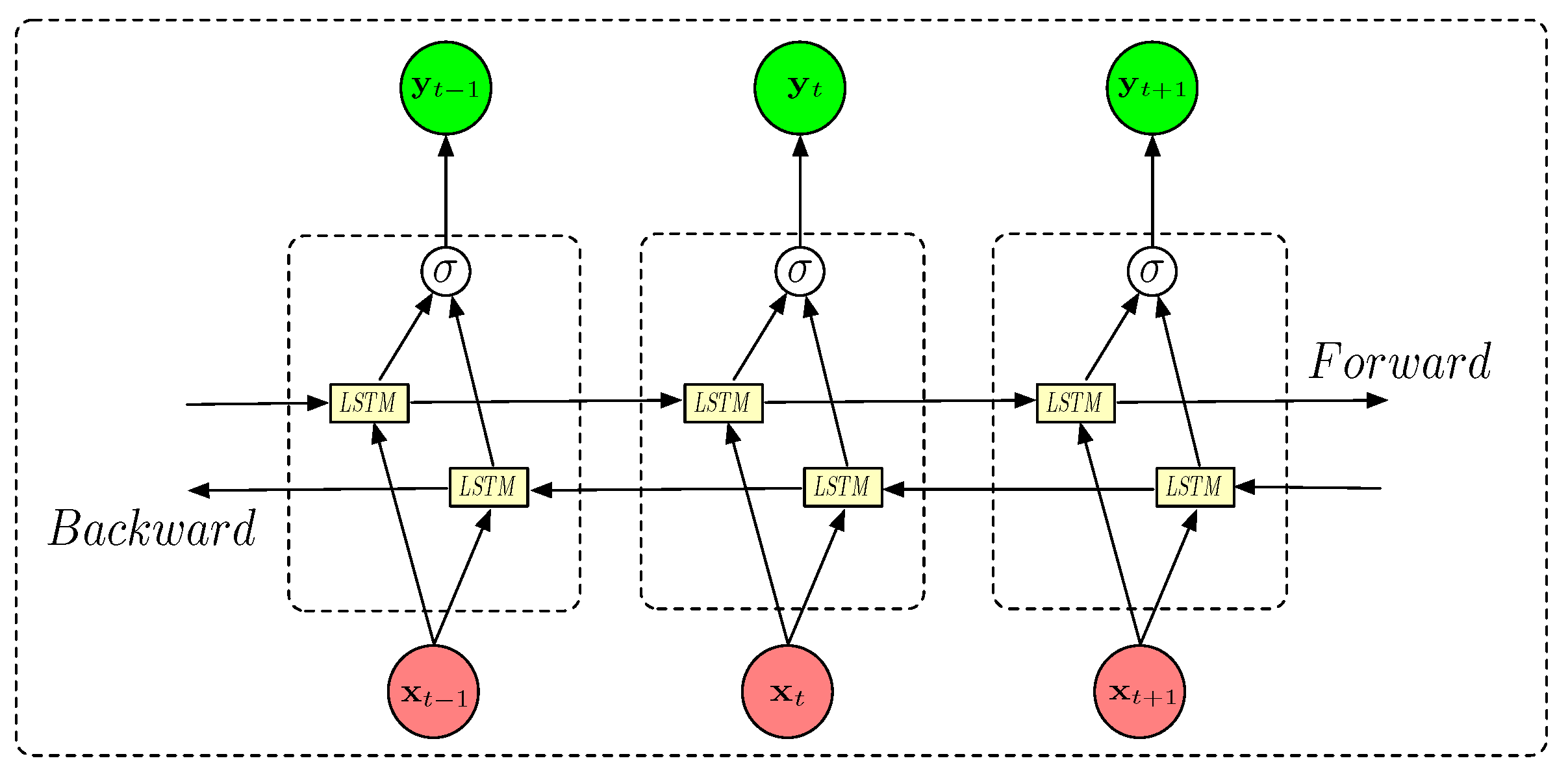
In applications such as analyzing EEG (electroencephalography) data for PD patients, a bidirectional LSTM (BDLSTM) model can be particularly effective. EEG data are non-stationary and often reflect complex brain dynamics that depend on past and future contexts. For instance, some EEG patterns, like event-related potentials (ERPs) or specific oscillatory activity (e.g., alpha, beta rhythms), depend on contexts that can be far away in time, both before and after a certain event. BDLSTM processes the data in both directions, forward (past to present) and backward (future to present), which helps the model to understand dependencies that span the entire signal window. This makes it well-suited to capture complex patterns in brain signals associated with the disease [23].

The BDLSTM architecture comprises two separate LSTM layers: a forward LSTM layer and a backward LSTM layer:

• The forward layer processes data from the beginning to the end of the signal sequence, with its output ${\overrightarrow{\mathbf{h}}}_t$ being iteratively calculated based on inputs ordered as ${\mathbf{x}}_1,{\mathbf{x}}_2,\cdots ,{\mathbf{x}}_T$.
• The backward layer processes data in reverse order, with its output ${\overleftarrow{\mathbf{h}}}_t$ being iteratively calculated using inputs ordered from time step T to time step 1; ${\mathbf{x}}_T,{\mathbf{x}}_{T-1},\cdots ,{\mathbf{x}}_1$.

The output of the BDLSTM layer is calculated using Equation (7), where ⊕ denotes the average of the forward and backward predictions.

$$y_t=\oplus ({\overrightarrow{\mathbf{h}}}_t,{\overleftarrow{\mathbf{h}}}_t)$$

(7)

This architecture is illustrated in Figure 4.

This design enables the model to process EEG signals in both the forward and backward directions. Thus, the model effectively utilizes information from the entire sequence at each time point, allowing for deeper analysis of Parkinson’s-related patterns that may not be detectable when relying solely on past signals. In sequence prediction tasks, a commonly used loss function is the mean squared error (MSE), defined as follows:

$$MSE={\displaystyle \frac{1}{n}}\sum _{i=1}^n{(y_{ai}-y_{bi})}^2$$

(8)

where:

• n: number of data samples.
• $y_a$: current predicted output.
• $y_b$: model prediction.

3. Methodology

This section includes a description of the dataset used in the experimental work, the way data are preprocessed, and the main training parameters.

3.1. Dataset

The UC San Diego Resting State EEG Dataset comprises EEG signals recorded from both PD patients and healthy individuals. The data were collected at the University of California, San Diego, and curated by Alex Rockhill at the University of Oregon [24]. EEG recordings were obtained using a 40-channel sensor system with a sampling frequency of 512 Hz. The dataset includes signals from 31 participants: 16 healthy individuals and 15 untreated PD patients. Each signal’s length ranges from 92,672 to 149,504 samples, with a total of 1240 signals across all participants. To generate synthetic signals, a BDLSTM model was trained on 98% of each signal, reserving the remaining 2% (typically exceeding 2000 samples) for validation.

3.2. Preprocessing

Since most relevant brain activity is found in the 0.5 Hz to 40 Hz range in the power spectrum of EEG signals, the original data were filtered using a bandpass filter with low and high cutoff frequencies of 0.5 Hz and 50 Hz, respectively. As the sampling frequency was 512 Hz, the signal spectrum contains information up to a maximum frequency of 256 Hz. In this way, the bandpass filtering effectively eliminates high-frequency noise while preserving the frequencies of interest. Signals captured by the sensors outside this bandwidth are generated by other sources, such as the heart and muscles, which can obscure brain signals and make their detection more difficult.

Muscle and eye movement artifacts were retained, as movement-related information may be relevant for PD detection, since PD symptoms are often associated with motor impairments. There are studies where artifacts in EEG signals are intentionally retained for PD analysis, particularly when these artifacts may carry diagnostic information. For instance, a study by Weyhenmeyer et al. [25] demonstrated that muscle artifacts present in raw EEG data could enhance the classification accuracy between PD patients and healthy individuals. They found that raw EEG data that included muscles artifacts yielded better classification performance compared to cleaned EEG data. This suggests that muscle artifacts may contain valuable information for distinguishing PD patients from healthy controls. Similarly, a systematic review by Maitin et al. [26] highlighted that some studies opted not to remove artifacts from EEG signals, recognizing that certain artifacts might be informative for PD detection. This approach underscores the potential diagnostic value of retaining specific artifacts in EEG analysis for PD. These examples illustrate that, depending on the research objectives, retaining certain artifacts in EEG data can be a deliberate and informative strategy in PD studies.

After bandpass filtering, all channels were considered in this study. This process effectively reduces noise while preserving essential signal information for training the models. Our goal was to develop a data augmentation method capable of generating signals that closely resemble those obtained in real-world systems.

After that, the data were normalized to ensure the dynamic range was consistent across all cases and to avoid any dependence of the results on the acquisition system’s gain. Z-score normalization was not used in this work, as this is typically applied to Gaussian-distributed signals to achieve zero mean and unit variance. However, it does not necessarily constrain the dynamic range to [−1, 1].Therefore, we opted for the normalization described in Equation (9), which ensures that the outputs are within the [−1, 1] range, as we believe this is more suitable for training machine learning systems. In expression (9), $X_{max}$ and $X_{min}$ denote the maximum and minimum signal amplitude values, respectively.

$$X^{\prime }=2\left({\displaystyle \frac{X-X_{min}}{X_{max}-X_{min}}}\right)-1$$

(9)

3.3. Training

The main objective is to use an LSTM neural network to predict samples of EEG signals. The model was trained to minimize the MSE between the original and the synthetic signal, generated with the LSTM neural network.

A neural network based on BDLSTM cells was used because it could learn from patterns in both directions across the time series. This approach enhanced the model’s ability to understand temporal relationships by analyzing preceding temporal contexts.

The number of epochs was determined through validation. Training was performed in epochs, and the segments used for validation measured model performance and halted training when the validation error increased. Performance improved until the number of epochs was 24, where the approximation error reached a minimum, which remained stationary in many cases but worsened in some channels due to overfitting. The number of epochs was set to 24, as fewer epochs resulted in suboptimal training, while more led to overfitting in some channels. The Adam optimization algorithm was used for training, with a learning rate ${10}^{-3}$. Although the learning rate could be selected using various tools (e.g., using lr_range_test in PyTorch since version 1.0 or tf.keras.callbacks.LearningRateScheduler) or selected using, for example, Bayesian optimization, we chose a commonly used value from the literature to focus on optimizing the network structure, reserving detailed parameter optimization for future studies. Additionally, for training, the signals were divided into smaller sequences with a batch size of 100 samples. Other batch sizes showed no significant change in the results.

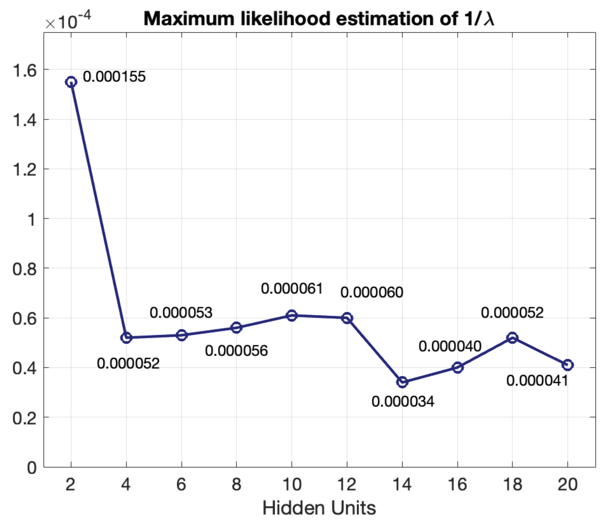
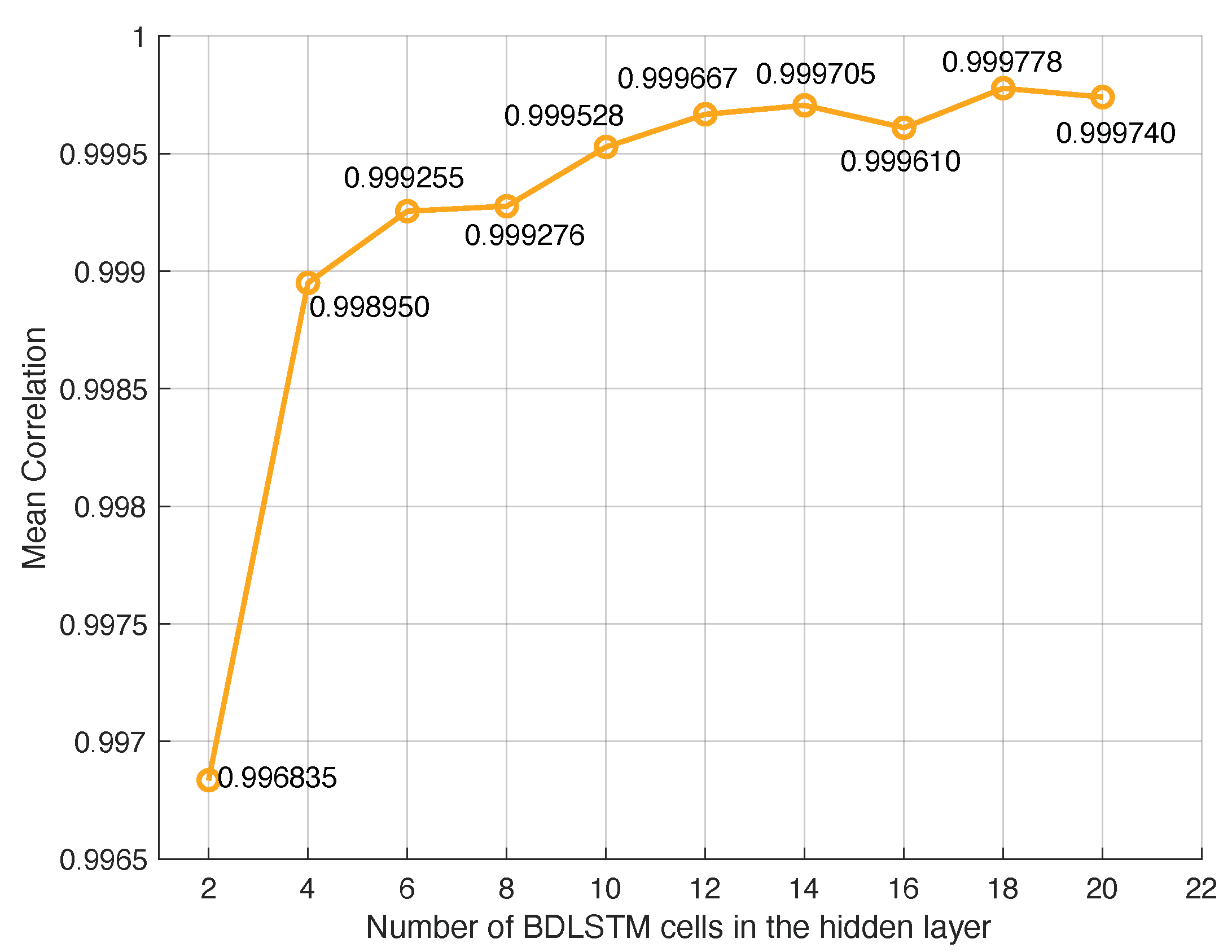
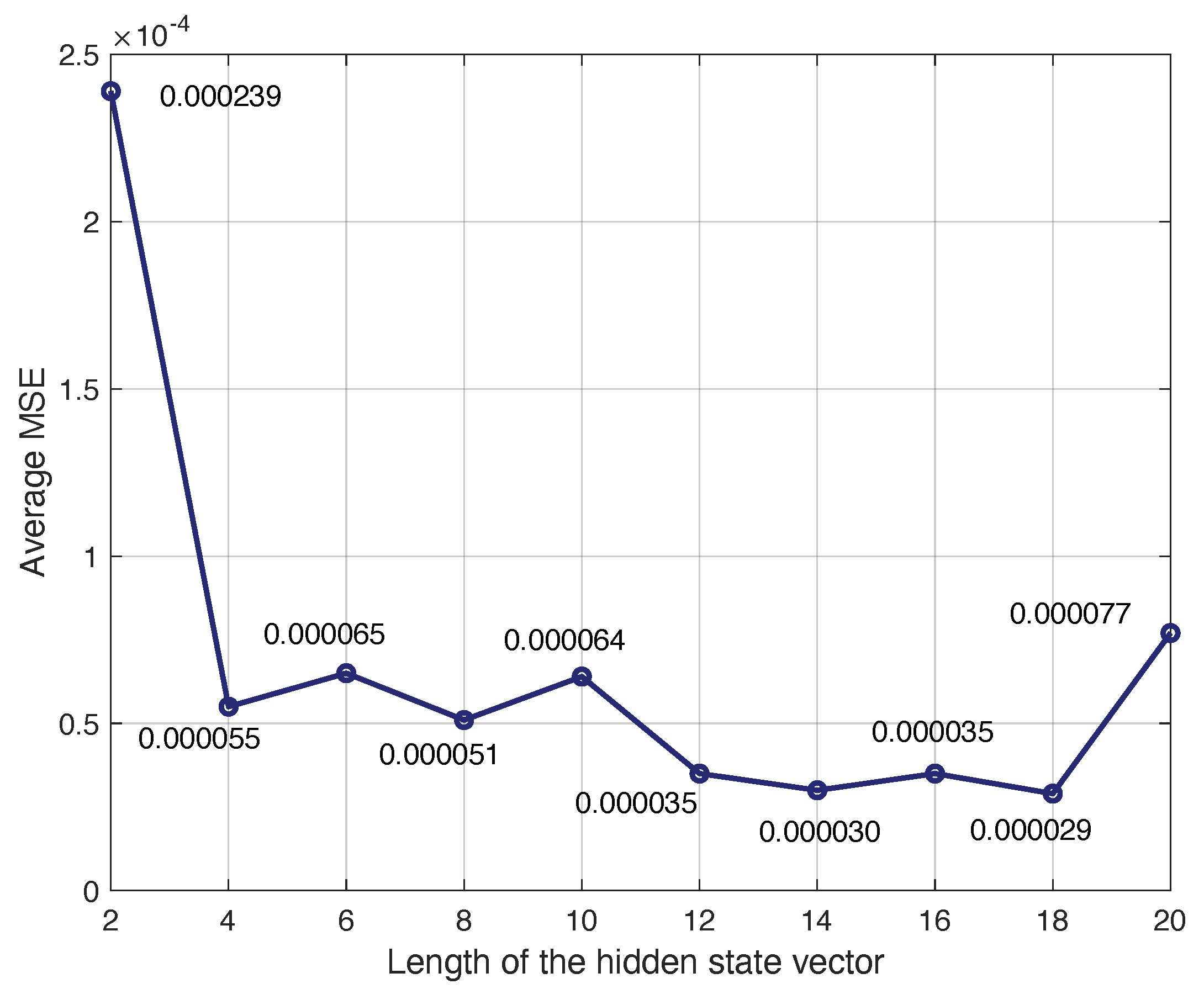
The number of BDLSTM cells in the model was determined empirically by evaluating the model with increasing numbers of cells in the hidden layer and measuring the MSE between the original and the synthetic signal and the Pearson’s correlation coefficient.

The main parameters used during training were as follows:

• The cost or error function used for training was the mean square error (MSE).
• The model was trained with the back propagation (BP) algorithm. The learning rate for the BP algorithm was set to ${10}^{-3}$.
• The training dataset was split into two subsets, one with 98% of the available data used for training, and the remaining 2% were used for testing.
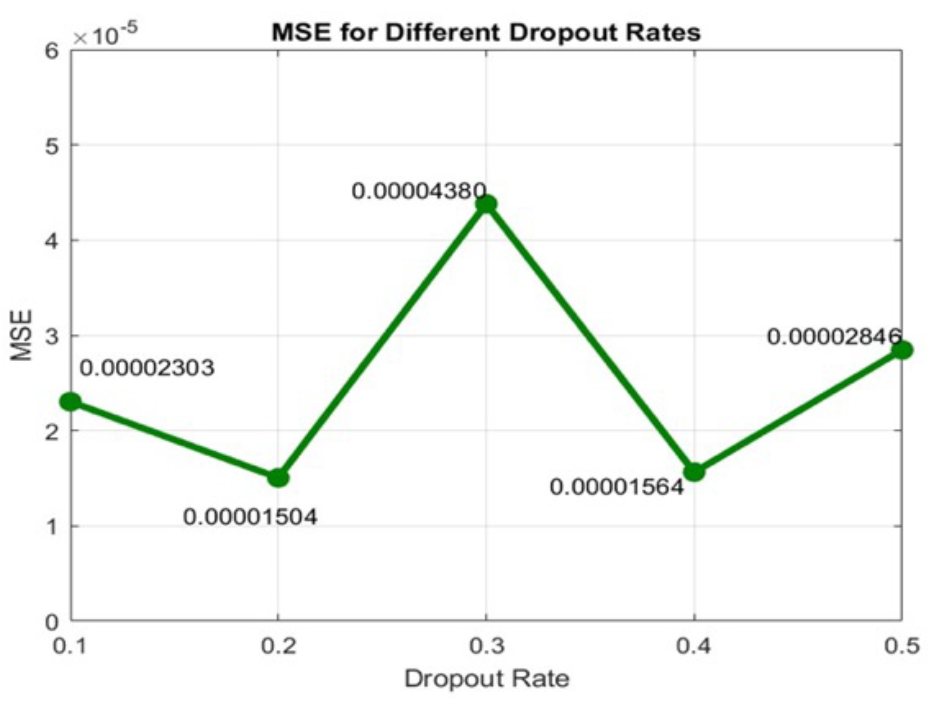
• We used a dropout layer, which is useful to reduce high data flow within a neural network and to prevent overfitting. Dropout is a regularization technique that probabilistically excludes input and recurrent connections to LSTM units from activation and weight updates during training. This has the effect of reducing overfitting and improving model performance. The dropout rate in training an LSTM model typically ranges from zero to one, where zero means no dropout (i.e., the network uses all neurons during training), and one indicates dropping out all the neurons (which is not effective for training). Given the small size of our dataset, lower dropout values were preferred to retain sufficient information. A grid search was implemented, testing different dropout values (0.1, 0.2, 0.3, 0.4, and 0.5). Figure 5 shows the MSE obtained with the BDLSTM models, comparing the original and synthetic signals across different dropout rates. The results indicate that while dropout improves performance, the optimal rate is 0.2, which we selected for our study.
• We also used the hyperbolic tangent (tanh) activation function, which is a commonly used activation function in neural networks, especially in hidden layers. The tanh function is especially useful if we have values ranging from $-1$ to 1.

4. Experiments and Results

Several experiments were carried out to decide which was the best structure based on BDLSTM cells to predict the EEG signals. Additionally, ARMA models were used as baseline for comparison purposes.

4.1. Baseline Model

Statistical models were utilized to compare the results of time series prediction with those obtained using BDLSTM models. Specifically, ARMA models were utilized, with the orders of the autoregressive and moving average components (p and q) determined experimentally through grid search. The Akaike information criterion (AIC) [27] was used as a statistical metric to compare and select the best-fitting model among a set of candidate models. It balances goodness of fit and model complexity by penalizing excessive parameters to prevent overfitting, and it is calculated using Expression (10):

$$AIC=2k-2ln\left(L\right)$$

(10)

where k is the number of parameters in the model, and L is the maximum likelihood of the model. A lower AIC value indicates a better model because it suggests a good fit with fewer parameters.

The average values of the AIC in the grid search to find the best AR and MA orders of the ARMA model (p and q, respectively) are depicted in Figure 6. The average AIC value presents an asymptotic trend, with a flat area observed, suggesting that the statistical models within this flat area perform similarly. We have selected the model with $p=9$ and $q=9$, as reference.

Figure 7 depicts one validation segment (in red) and the predictions made with that ARMA model. It can be observed that the ARMA model smooths the signal, obtaining a kind of time-averaged signal. Furthermore, it fails to follow sudden changes in the signal. Because of that, the Pearson correlation coefficient and the mean squared error values are far from the good ones obtained for the BDLSTM models. Specifically, Pearson’s correlation coefficient takes the value 0.5877, and the root mean square error value, MSE = 0.0373, both of which are significantly higher compared to the values obtained for the BDLSTM models.

4.2. Number of Cells of the BDLSTM Neural Network

The BDLSTM base model was trained and evaluated using an increasing number of hidden units in the hidden layer. The mean squared error (MSE) and the correlation between the synthetic and original signals were assessed using the test dataset across all subjects. The MSE decreased as the number of hidden units increased up to approximately ten units in all cases. Concurrently, the correlation between the synthetic and original signals increased, also exhibiting asymptotic behavior.

Additionally, we analyzed the statistical distribution of the MSE estimations for a given number of hidden units. We found that the MSE distribution aligned well with the exponential distribution, and its parameter could be estimated using the maximum likelihood estimator (MLE):

$$\widehat{\lambda }={\displaystyle \frac{n}{{\sum }_{i}MS{E}_i}}$$

(11)

Figure 8 illustrates the variation in the inverse of the estimated parameter ($1/\lambda$) of the exponential probability density function. These data correspond to channel F7 from a group of 31 individuals, including both untreated PD patients and healthy controls. As $1/\lambda$ decreases, the MSE also decreases, indicating improved signal estimation performance.

Figure 9 depicts the mean correlation coefficient between the signal from channel F7 of the group of 31 people in the database and its prediction using the BDLSTM-based neural network across the same group. The correlation exhibits asymptotic behavior, reaching a plateau when the number of BDLSTM cells is 10.

Analysis of the MSE reveals optimal results with 14 hidden units. In contrast, the correlation coefficient remains high even with a minimal number of hidden units, particularly exceeding 12 units, with only marginal improvements thereafter. Therefore, 14 units were selected, balancing superior MSE and correlation coefficient outcomes.

4.3. Length of the Hidden State Vector ${\mathbf{h}}_t$

The length of the hidden state vector determines the number of previous samples in the time series used to predict the current sample. The optimal length was determined experimentally by measuring the mean squared error (MSE) and correlation as the length varied. In these experiments, we used the previously established number of hidden units (14 units in the hidden layers). Figure 10 and Figure 11 show the average MSE and correlation obtained as the length of ${\mathbf{h}}_t$ increased. It was observed that the mean MSE decreased to a minimum value when the length was 4. Beyond this point, further increases in length resulted only in slight reductions in MSE, which did not justify the additional computational resources required. Similarly, the correlation reached a high value at a length of 4. Therefore, a length of 4 was selected for generating synthetic EEG signals in our model.

4.4. Discussion

The MSE was selected as metric to compare the similarity between the original and synthetic signals because it provides a quantitative measure of the average squared difference between corresponding points in the signals. MSE calculates how far, on average, the values of one signal deviate from the values of another. Since MSE squares the differences, larger deviations are penalized more than smaller ones, making it effective in detecting significant discrepancies. MSE is particularly useful for comparing time-domain signals where differences in amplitude matter, and it is computationally simple.

Table 1. Performance comparison between ARMA and BDLSTM models based on MSE, Pearson’s correlation coefficient, and architecture complexity.

Model	MSE	Correlation	Architecture
ARMA(p, q)	0.03731	0.5877	AR order, $p=9$; MA order, $q=9$
BD-LSTM	0.00006	0.9995	14 BD-LSTM cells; hidden state length ${\mathbf{h}}_t=4$

presents the average MSE and Pearson’s correlation coefficient, along with a brief description of the architecture for the selected ARMA model and the BD-LSTM-based neural network. The results obtained with the BD-LSTM model outperform those of the ARMA model, although the complexity is higher. To assess the importance of complexity, it should be noted that once the model is generated, it will be used to produce a synthetic database, which in turn will be used to train and test a detection system. The detection system may indeed have strict real-time performance requirements, but in the case of the model used to synthesize signals, it is far more important that the signals produced are useful.

Nevertheless, the MSE or the Pearson’s correlation coefficient do not capture the quality of the generated signals visually. For a complete comparison, Figure 12 shows the waveforms of four segments of one EEG signal and the synthetic versions generated with the trained BDLSTM model, demonstrating how close the synthetic versions are to the original ones.

Additionally, we compared the power spectra of the original and synthetic signals. As one power spectrum estimator that is more commonly used is the Periodogram, which is by nature random with a variance proportional to the squared value of the power spectrum, or statistical models, such as AR, MA, or ARMA, which can only model the envelope of the power spectrum, we used a different method for the comparison. The aggregated power in the frequency bands usually used with EEG signals was calculated. The power in these bands is used to evaluate the information contained EEG signals and even to calculate it. A similar power in these bands indicates similar information content.

Table 2. Power spectral density comparison of the original and synthetic signals in the delta, theta, alpha, beta, and gamma bands used in EEG analysis.

Frequency Band	Original Signal	Synthetic Signal
Delta	0.0127	0.0121
Theta	0.012	0.012
Alpha	0.0010	0.0010
Beta	0.0029	0.0028
Gamma	0.0028	0.0030

presents the estimated values of power in the delta, theta, alpha, beta, and gamma bands for both the original and synthetic signals, demonstrating very similar values.

Therefore, the results obtained demonstrate that it is possible to generate EEG signals very similar to the original ones using a neural network with a single layer of BDLSTM cells. The comparison between the original and the synthetic signals was performed using MSE, the Pearson correlation coefficient, and the powers in the bands usually employed in the analysis of EEG signals.

5. Conclusions

This study addresses the challenge of generating synthetic EEG signals from PD patients as a data augmentation strategy. The demand for synthetic signals arises from the necessity of training deep learning neural networks to distinguish between individuals with PD and healthy subjects. Deep neural networks, particularly those with a large number of parameters, require substantial amounts of training data to prevent overfitting. However, acquiring large, high-quality datasets is often impractical, making data augmentation a crucial solution. The models developed in this study aim to generate synthetic signals to expand the training dataset, following the principles of data augmentation.

The practical significance of this research lies in its ability to offer innovative solutions to data scarcity—a challenge that impacts numerous fields, particularly medicine, where obtaining patient data is often complex, expensive, and time-consuming. The proposed methodology facilitates the generation of reliable synthetic datasets that can be leveraged for analysis and development without requiring additional data collection.

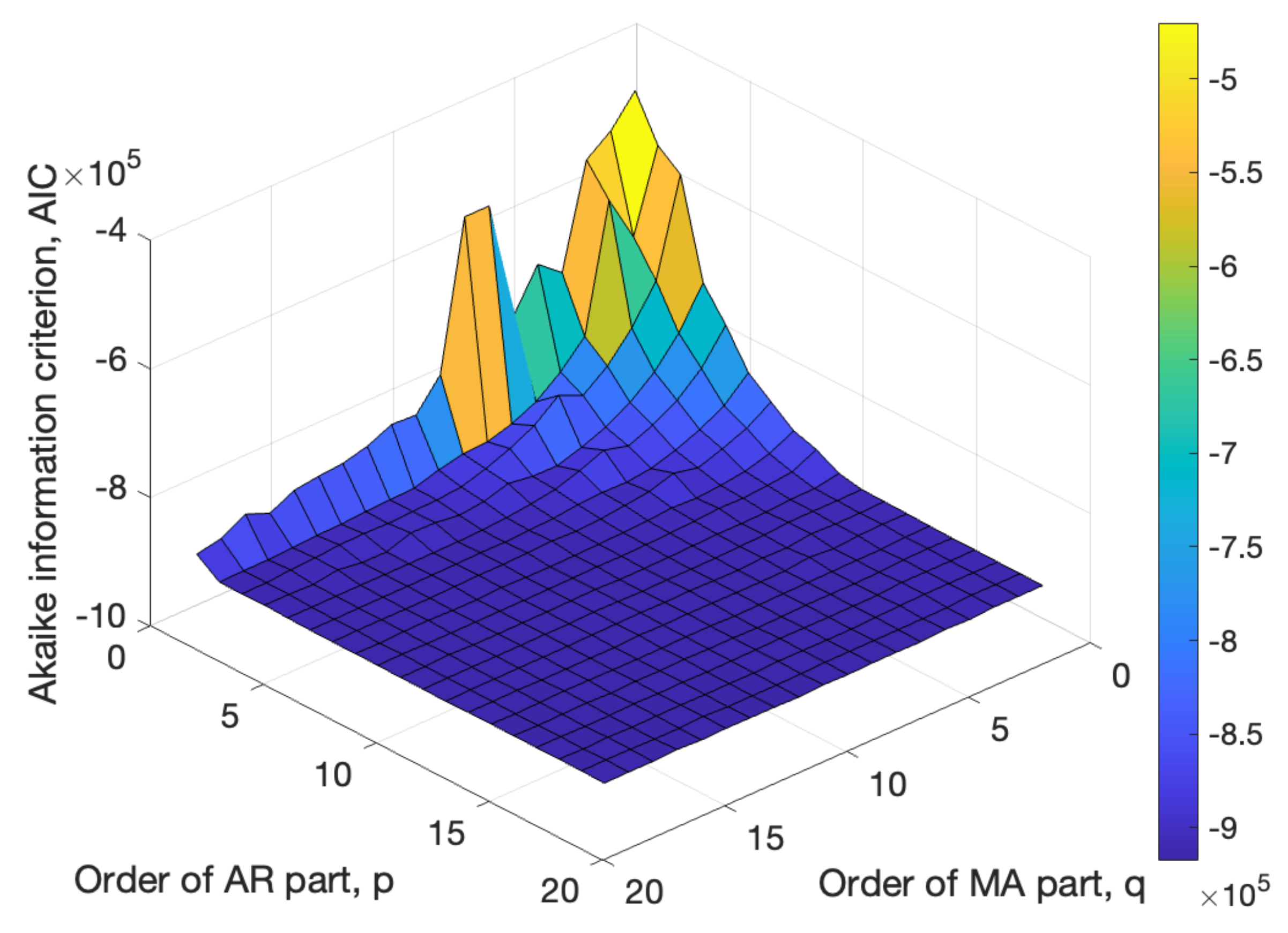
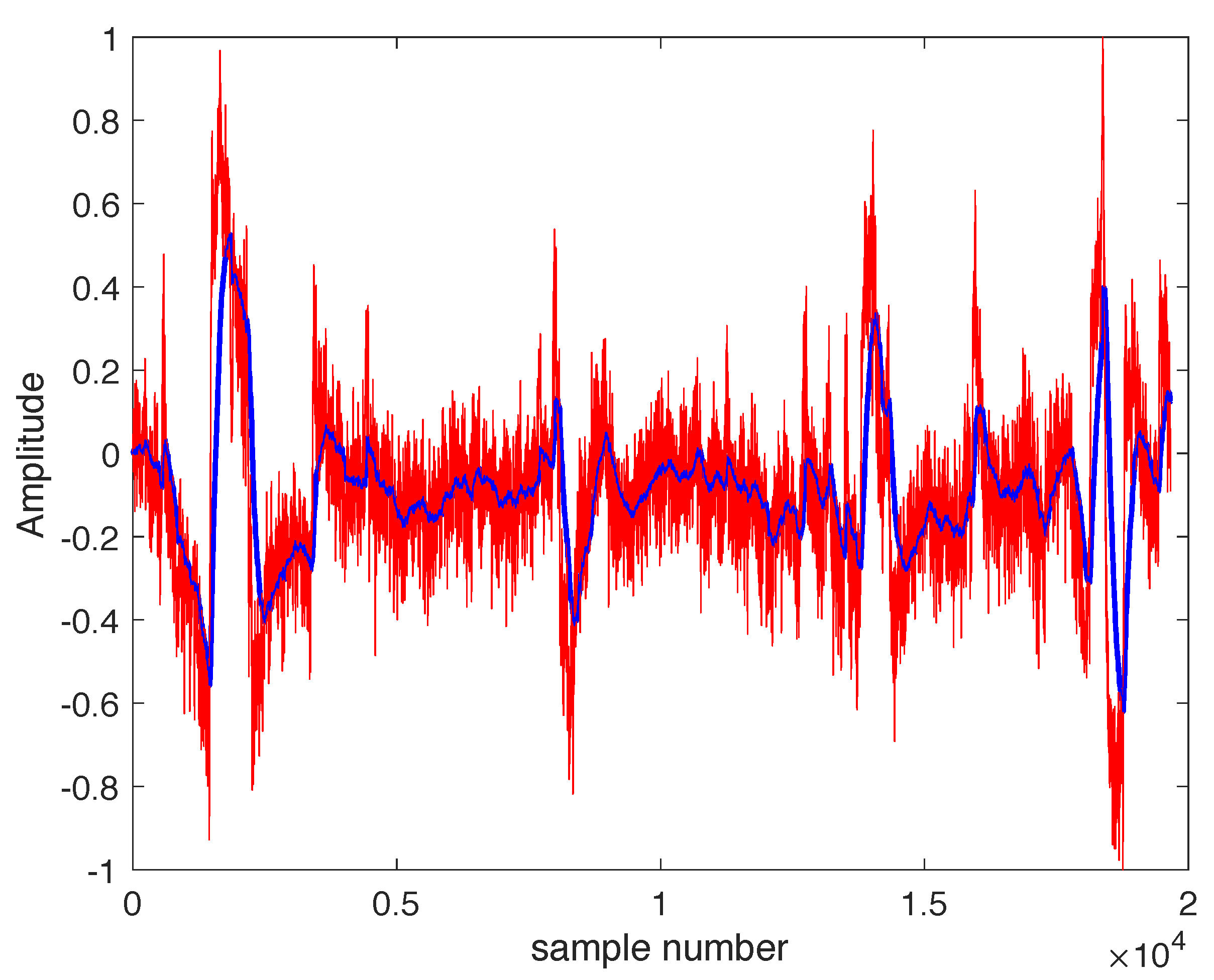
Traditional linear models, such as AR, MA, and ARMA, struggle to generate EEG signals while retaining all diagnostically relevant information. In this study, the feasibility of using ARMA models for synthetic EEG generation was explored. The optimal ARMA model was selected based on the Akaike information criterion (AIC) and model complexity. However, even the best-performing ARMA model produced a filtered version of EEG signals, losing high-frequency components that may hold diagnostic value. The experiments were conducted using EEG recordings from PD patients as the reference signals.

To overcome the limitations of linear models, a neural network incorporating BDLSTM units was implemented, demonstrating superior performance. This constitutes a key contribution of this research, as BDLSTM-based neural networks have not previously been applied to generating EEG data for PD patients.

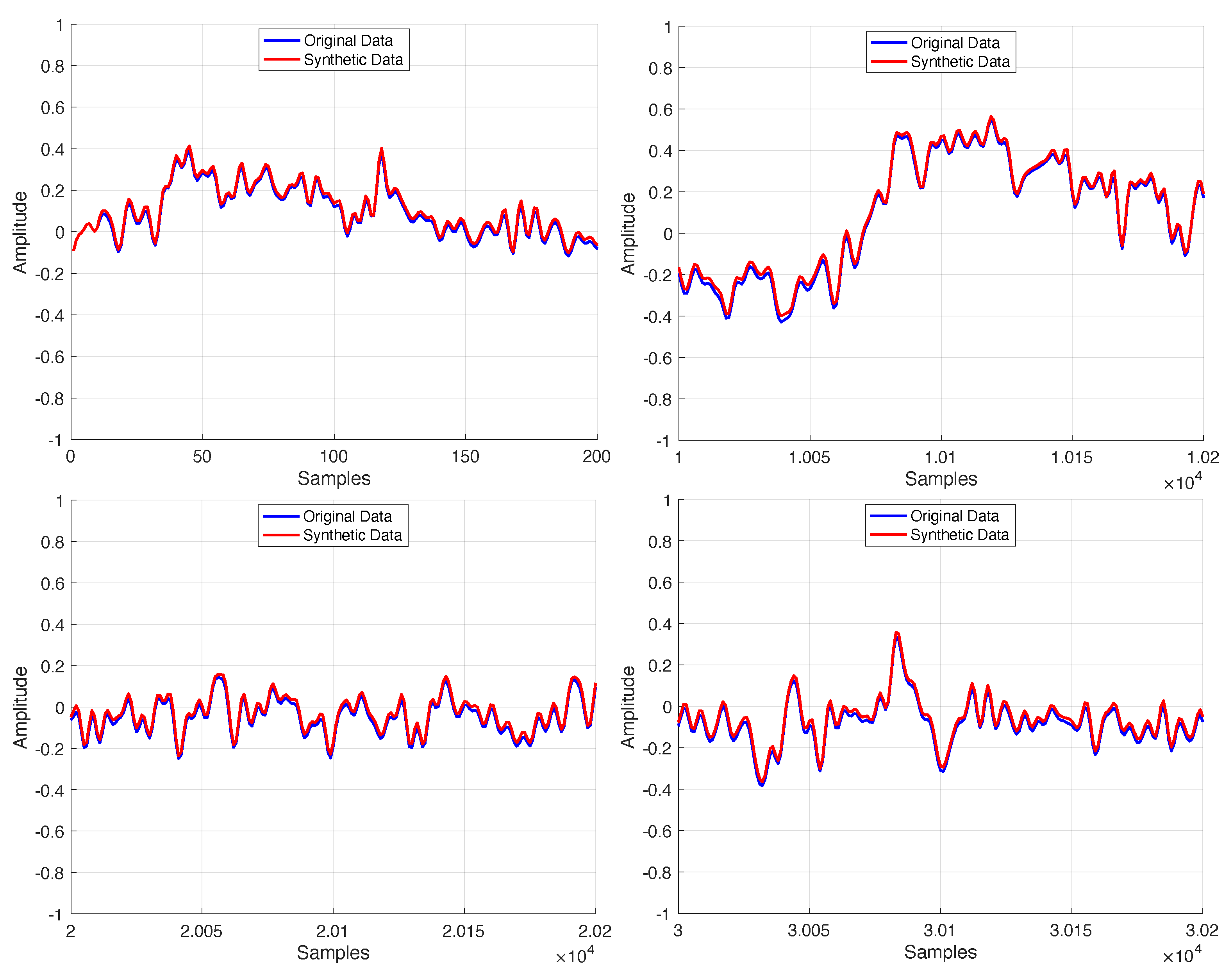
The proposed model is a neural network with a single hidden layer, consisting of an optimized number of BDLSTM cells, each with an ideal hidden state vector length. A separate model was trained for each available signal in the dataset, demonstrating that, after optimization, the results remained consistent across all signals. This approach aims to develop a compact, low-complexity neural network based on BDLSTM cells, making it suitable for integration into more advanced architectures, such as GANs, where optimization processes are inherently more challenging. This novel methodology has led to a highly effective system capable of generating synthetic signals that closely resemble the original ones, particularly in non-linear time series. Performance was evaluated using mean squared error (MSE) and Pearson’s correlation coefficient, confirming the model’s ability to preserve essential signal characteristics. Consequently, the optimization process strikes a balance between model complexity and accuracy, reducing computational costs while ensuring the generated synthetic samples maintain the statistical properties of the original measured signals.

This study also revealed certain limitations and uncertainties that should be considered in future research. Firstly, the validity of the synthetic databases needs to be assessed; to this end, we intend to conduct a study in which detectors will be trained and tested on real data. Furthermore, although previous studies suggest that it may be preferable to retain movement-related artifacts in EEG signals, it is still necessary to evaluate whether keeping this information is beneficial or whether it is, in fact, better to remove it. For now, the proposed model allows this information to be retained, with the understanding that artifact removal algorithms can be applied later to the synthetic signals if needed.

The designed models allow for the synthesis of signals with characteristics very similar to those used for training, which may not be effective for expanding datasets. For the effective training of detectors, the generated signals must be diverse, so efficient strategies need to be developed to introduce variability. This aspect goes beyond the scope of this article, but some possibilities to explore include using the signals from one patient with another patient’s model to generate hybrid information or introducing time warping into the synthetic signal. This is a line of research that should be addressed in the near future.

Beyond its medical applications, this study introduces powerful tools with implications across multiple disciplines, from engineering and data science to financial modeling. By leveraging this technology, researchers can generate highly accurate synthetic data, advancing the understanding of natural, economic, and social phenomena. This, in turn, facilitates scientific discovery, fosters innovation, and enables researchers to tackle challenges that were previously insurmountable.

Several promising research directions emerge from this work. First, the generated synthetic signals will be used to train PD detection systems. The augmented dataset is expected to mitigate overfitting, allowing the original data to be reserved exclusively for testing, leading to more reliable model evaluations.

Second, and equally important, is the exploration of more advanced architectures, such as generative adversarial networks (GANs), where the generator could be built upon the optimized model presented in this study. The competitive nature of GANs, wherein the generator and discriminator iteratively refine each other, has the potential to enhance the quality of synthetic signals. However, the challenges associated with training GANs for time series generation warrant further investigation.

Third, this approach should be extended to other biomedical datasets that are challenging to obtain and could benefit from effective data augmentation techniques. These include electrocardiogram (ECG) signals, electromyography (EMG) signals, heart rate variability (HRV), and blood pressure (BP) signals. Additionally, human activity-related time series, such as motion tracking and walking pattern data used for behavioral anomaly detection, could also be considered.