Carrot Yield Mapping: A Precision Agriculture Approach Based on Machine Learning

Abstract

Carrot yield maps are an essential tool in supporting decision makers in improving their agricultural practices, but they are unconventional and not easy to obtain. The objective was to develop a method to generate a carrot yield map applying a random forest (RF) regression algorithm on a database composed of satellite spectral data and carrot ground-truth yield sampling. Georeferenced carrot yield sampling was carried out and satellite imagery was obtained during crop development. The entire dataset was split into training and test sets. The Gini index was used to find the five most important predictor variables of the model. Statistical parameters used to evaluate model performance were the root mean squared error (RMSE), coefficient of determination (R²) and mean absolute error (MAE). The five most important predictor variables were the near-infrared spectral band at 92 and 79 days after sowing (DAS), green spectral band at 50 DAS and blue spectral band at 92 and 81 DAS. The RF algorithm applied to the entire dataset presented R², RMSE and MAE values of 0.82, 2.64 Mg ha⁻¹ and 1.74 Mg ha⁻¹, respectively. The method based on RF regression applied to a database composed of spectral bands proved to be accurate and suitable to predict carrot yield.

1. Introduction

Yield maps are one of the most used features in precision agriculture (PA) [1]. PA is a management strategy that assists decision makers by leveraging predicted variability from the collected, processed and analyzed spatial, temporal and individual data [2]. PA aims to improve resource use efficiency, yield, quality, net economic return and sustainable production [2].

Yield maps can be generated from data collected through different harvesting systems: (a) manually harvested (citrus and horticultural crops [3]) and (b) mechanically harvested (data from yield monitors, for example, in soybean and corn [4]). Yield mapping from manually harvested data is challenging since the harvesting process is highly laborious yet produces better sampling quality [5]. On the other hand, yield mapping from yield monitors that collect high-density data with less human labor is limited by several factors that affect data quality such as the need for constant inspection of the sensor system and calibration before and during the harvesting process [6].

Data quality is one of the key features that determines the accuracy and correct interpretability of the results, and this topic has already been explored by [7]. In the era of big data, massive volumes of highly varied data can be obtained, analyzed and used to support decision-making [8]. Hence, machine learning (ML) presents itself as a potential tool in identifying rules and patterns in these kinds of datasets [9] that can cope both with linear and non-linear problems [10].

In this light, remote sensing (RS) becomes a suitable alternative in assessing yield maps instead of using yield monitor data [11,12], where data is compromised by sensor system factors such as inappropriate calibration [6]. RS generates sufficiently large amounts of data to be considered big data [13]. RS techniques provide instantaneous, non-destructive, quantitative information on crop conditions and yield estimation [14,15,16]. RS imagery is commonly applied to forecast annual crop yield as an alternative to yield monitors. However, few studies have investigated the use of RS imagery to estimate yield for horticultural crops [12].

The use of yield maps is widespread for annual crops such as corn and soybean [4], yet this technique remains unutilized for horticultural crops like carrots, even though it is known that yield mapping provides beneficial data to support decision makers [17]. As carrot crops present high economic value, efforts to optimize its crop management based on PA techniques are justified, for example, by applying site-specific management [17].

Different approaches to estimate crop yield have been developed, and the application of ML algorithms on databases composed of vegetation indices (VIs) derived from satellite imagery data is being largely adopted [18,19,20,21]. The random forest (RF) algorithm currently stands out among the others in predicting crop yield on datasets composed of VIs (sunflower [22], sugarcane [23], and rice [24]) or spectral bands (corn [25]). Using ML to predict yield from VIs has shown potential in discovering new interactions [9]. It is thus important to look for similar methods in predicting yield based on spectral bands, as there is still a lack of knowledge on how they relate to crop production.

Given the lack of yield map availability for horticultural crops [12], especially for carrot crops, and keeping in mind the existence of methods to generate yield maps from manually harvested crops [3], it is also important to look for alternatives that will allow carrot farmers to have access to yield maps similar to what has been done for citrus crops [26].

As technology advances in agriculture, with high-performance computers becoming the norm, machine learning techniques becoming more popular and satellite imagery data becoming easily accessible, there is opportunity to develop fast, accurate and reliable methods in generating carrot yield maps based on (a) spectral data from satellite imagery instead of VIs, (b) on-field punctual carrot yield sampling (ground-truth) and (c) the application of a random forest regression algorithm. Hence, the objective of this work was to develop a method to generate carrot yield maps by applying an RF regression algorithm on a database composed of raw spectral data from satellite imagery and on-field carrot yield sampling data to further extrapolate the fitted model to larger carrot cultivated areas.

2. Materials and Methods

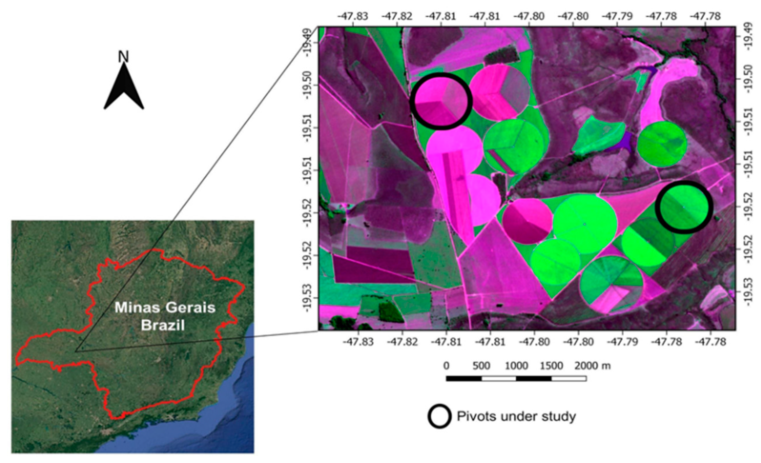
2.1. Study Site

This study was carried out during the 2017 crop season in two irrigated agricultural fields with a central pivot located in Uberaba (19°31′7″ S and 47°46′45″ W), state of Minas Gerais, Brazil (Figure 1). The site has a tropical climate classified as Aw (Koppen-Geiger classification) with an annual average precipitation, temperature and altitude of 1571 mm, 22.3 °C and 789 m, respectively. Carrot (cv. Verano) was mechanically seeded in May 2017. The soil was previously prepared with one plowing and two harrowing procedures. Carrot seeding was done in beds of 1.75 m width, and seed deposition was arranged in three sets: triple rows at each of the edges and double rows at the central position. Carrot harvesting was initiated in August 2017.

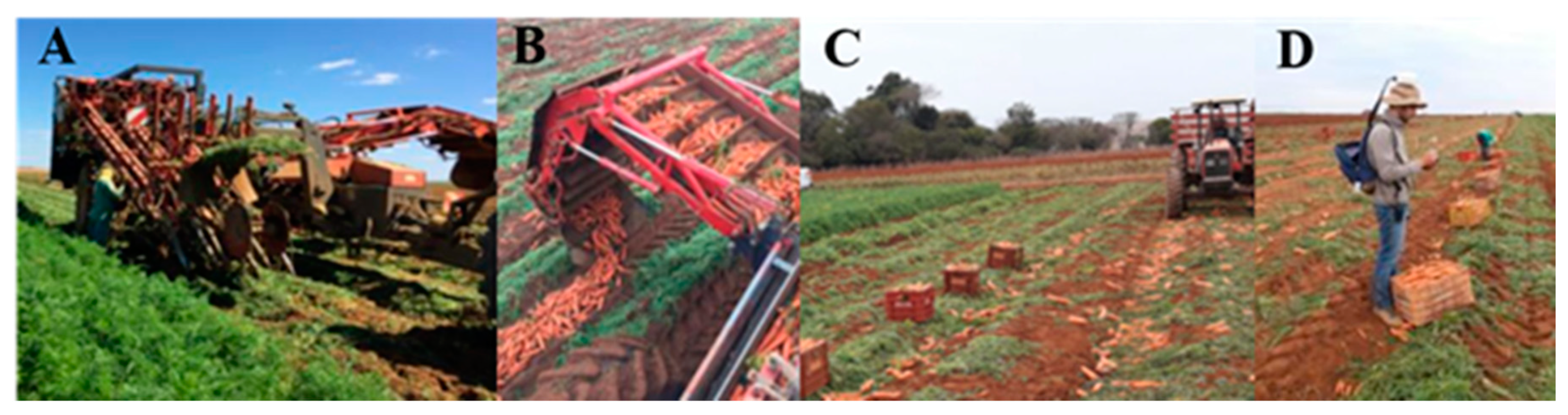
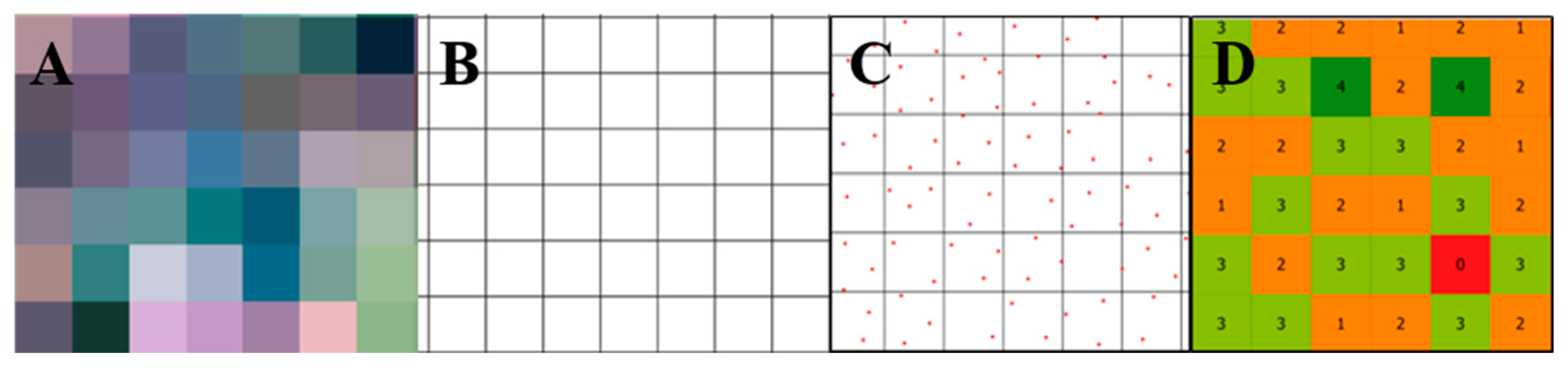
2.2. Harvesting and Yield Mapping

A semi-mechanized carrot harvesting system was used in this study as shown in Figure 2. The harvester (Figure 2A), a Dewulf GKIIISE (Dewulf Group, Roeselare, Belgium), harvests the carrot roots, removes the soil, cuts the leaves and places the carrots on the left side of the harvester with 5.25 m displacement (Figure 2B). As the harvester machine travels through the field, carrots are collected and displaced 16.5 m ahead of the point where they were initially taken. To account for this, an offset was applied to adjust the sample deposition location. The harvesting operation was carried out in a single direction due to the operating mode of the harvester. This resulted in systematic root deposition errors throughout the entire harvesting path. These positioning errors were removed in a post-processing procedure. Pre-instructed collectors selected the roots according to market standards [27]. The roots that did not fit market standards were discarded in the field (Figure 2C) and the others placed in plastic boxes with dimensions of 0.30 m × 0.33 m × 0.55 m and capacity of 52 L. Following the methodology described by [3], which we adapted to the above conditions, all boxes in the field were georeferenced using a global navigation satellite system (GNSS) receiver, model SMART-AG (NovAtel Inc., Calgary, Canada) (Figure 2D).

Carrot yield map generation was carried out in three steps according to the methodology adapted from [3]. First, a layer was created using a regular polygon grid extracted from satellite imagery with a spatial resolution of 3 m × 3 m (Figure 3A and 3B). Second, the number of boxes in each pixel was counted (Figure 3C and 3D). Outliers were removed according to the method in [28]. Areas presenting missing values were estimated based on the mean value among their neighbors. As a result of the previous steps, a carrot box quantity map (box ha⁻¹) was made. Third, the carrot box quantity map was converted into a yield map (Mg ha⁻¹) by multiplying the number of boxes inside each pixel by the weight of one carrot box. The weight assigned to one carrot box was calculated by averaging the weight of 150 carrot boxes.

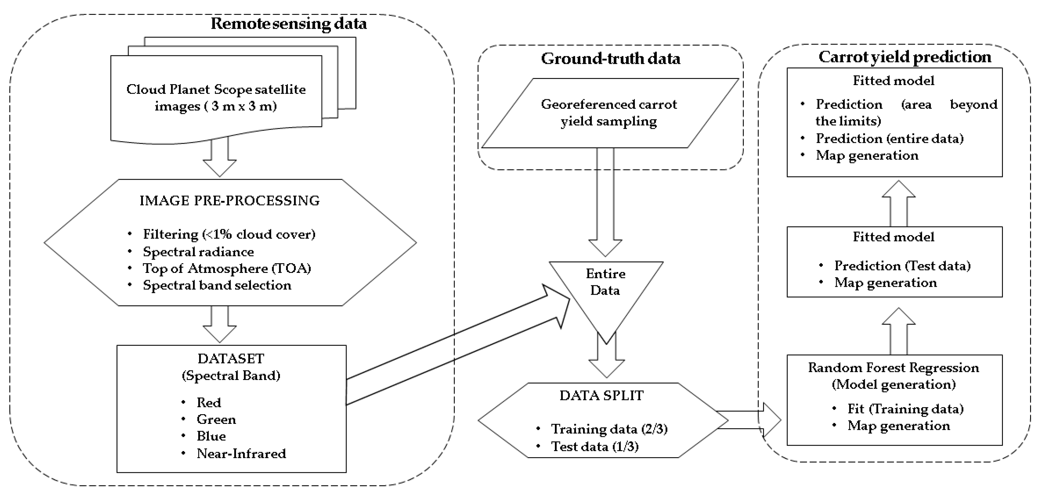
2.3. Satellite Imagery Data

Cloud Planet Scope satellite images (spatial resolution of 3 m × 3 m) were downloaded from the archives of the Planet website [29] for the study period from 1 May to 31 August of 2017. Images were collected from sowing to harvest period. The set of images was provided in 16-bit GeoTiff format, each containing four spectral bands: blue (B) (455–515 nm), green (G) (500–590 nm), red (R) (590–670 nm) and near-infrared (NIR) (780–860 nm). Data was received as an Ortho Scene product (level 3B), which relates to a top-of-atmosphere (TOA) reflectance suitable for analytic and visual applications. Then, a python algorithm to automatically correct the radiance and calculate the reflectance was adapted from [30] to work in the R environment. With this, each spectral band in the images was calibrated using the data-specific utilities of R v3.5.5 [31] software, in which the digital numbers of the sensor were converted into spectral radiance to measure the amount of electromagnetic radiation reflected from a spot on the surface. Spectral radiance (Lλ) was determined by applying the calibration coefficients from the image metadata [19]. Then, reflectance images were generated from the calculated radiance. Reflectance (dimensionless) is usually the ratio between the reflected and incoming radiance [31]. In this case, the reflectance was calculated through Equation (1), which is the TOA reflectance, not taking into account any atmospheric influence [32].

REF(i) = [RAD(i) π SunDist²] [EAI(i) cos(SolarZenith)]⁻¹

(1)

where REF = reflectance value, RAD = radiance value, i = number of the spectral bands, SunDist = Earth-Sun distance on the day of acquisition, EAI = exo-atmospheric irradiance, SolarZenith = 90°—sun elevation. Note that all these variables are available in the image metadata.

Images were chosen according to the sensor archive availability and cloud cover. All the images were acquired on days of low cloud cover (<1%). In this study, the spectral bands from the temporal stack were used as data input to analyze their relation with the ground-truth carrot yield data samples.

2.4. Dataset

On-farm punctual carrot sampling data was incorporated into the satellite imagery data with the same spatial resolution (3 m × 3 m). Each pixel contained (a) temporal spectral bands (red, green, blue and NIR) from the satellite images taken during the carrot growing period and (b) carrot yield observed values. This resulted in a dataset composed of 89 variables (one response variable and 88 predictive variables) and 15,093 sampling points. Furthermore, the data was divided into training (2/3) and test (1/3) datasets to apply the RF regression algorithm. After the application of the RF regression model to the training and test datasets, the fitted model was applied to the entire dataset as well as an area outside the ground-truth sampling region.

2.5. Random Forest Regression Prediction

RF regression is a combination of decision trees, where each tree depends on the values of a random vector sampled independently from the input vector with the same distribution for all trees in the forest [33]. According to [34], RF differs from single decision tree models because it relies on the average result of many trees (ntree).

RF regression was implemented in the R framework [31] with the randomForest package [35]. From this package, the randomForest() and predict() functions were used to fit the RF regression model and predict yield respectively. To improve the model accuracy, it was necessary to fine-tune some parameters (ntree and predictor subset value—mtry). Thus, a bootstrapping sample size equal to two-thirds of the entire dataset was used to grow each tree, and the remaining one-third was used to calculate out-of-bag (OOB) error. The set.seed(123) function was used to obtain reproducible results. The default predictor subset (mtry) value of the randomForest package [35] is typically equal to the number of predictors (p) divided by three. However, it is necessary to calculate the optimal mtry value since it depends on the data [36]. According to [33], RF can grow as many trees as desired and the results will not overfit. In contrast, [36] suggests that too many trees would result in a model that is too rich, which could increase variance and affect prediction accuracy. To mitigate this, the prediction error rates were calculated for the RF regression algorithm for each ntree value from 0 to 500. The ntree value that presented the lowest error before stabilization was selected. A mean decreased Gini index was applied to find the five most important variable predictors used by the model to estimate yield. Variable selection through a mean decreased Gini index has been largely applied in RF algorithms [37,38].

The performance indicators used to evaluate the model’s goodness of fit were the root mean squared error (RMSE—Equation (2)), coefficient of determination (R²—Equation (3)) and mean absolute error (MAE—Equation (4)) [19]. For each sampled point, the prediction error (the difference between the predicted carrot yield (Mg ha⁻¹) of the model and observed yield (Mg ha⁻¹)) and the absolute error percentage were calculated. Maps were made with Quantum Geographic Information System (QGIS) software [39].

RMSE = {n⁻¹ [∑(y_i – ŷ)² + … + (y_n – ŷ)²]}^0.5

(2)

where RMSE = root mean squared error, n = number of samples, y = observed variable response and ŷ = predicted variable response.

R² = 1− {[∑(y_i – ŷ)² + … + (y_n – ŷ)²] [∑(y_i – ӯ)² + … + (y_n – ӯ)²]⁻¹}

(3)

where R² = coefficient of determination, n = number of samples, y^.= observed variable response, ŷ = predicted variable response and ӯ = mean value of the observed response variable.

MAE = {n⁻¹ [∑(|y_i – ŷ|) + … + (|y_n – ŷ|)]}

(4)

where MAE = mean absolute error, n = number of samples, y = observed variable response and ŷ = predicted variable response.

A flowchart corresponding to the carrot yield prediction and mapping procedure is shown in Figure 4. It presents the process through the stages of data collection using satellite imagery (including pre-processing and data selection), georeferenced carrot yield sampling, data merging (satellite imagery and carrot yield sampling data), data splitting (train and test data) and RF regression application.

3. Results and Discussion

3.1. Harvesting and Yield Mapping

The descriptive statistics of the weight of 150 carrot root boxes are presented in

Table 1. Descriptive statistics of 150 boxes of carrot roots.

Min 1	Median	Mean a	Max 2	Standard Deviation b	CV 3,c
kg box−1					%
27.20	28.68	28.59	30.09	0.62	2.15

¹ Minimum, ² maximum, ³ coefficient of variance; ^a mean = [∑(y_i + … + y_n)] n⁻¹, ^b standard deviation (s) = {(n-1)⁻¹ [∑(y_i – ӯ)² + … + (y_n – ӯ)]²}^0.5, ^c CV = 100 s ӯ⁻¹, where y₁ = observed response variable, ӯ = mean value of the observed response variable and n = number of samples.

. It shows a standard deviation of 0.62 kg box⁻¹, a coefficient of variance of 2.15%, a minimum value of 27.20 kg box⁻¹, a maximum value of 30.09 kg box⁻¹, a median value of 28.68 kg ha⁻¹ and an average weight value of 28.59 kg box⁻¹. From this, a value of 28.59 kg was assigned to each carrot box to continue the procedure to generate carrot yield maps.

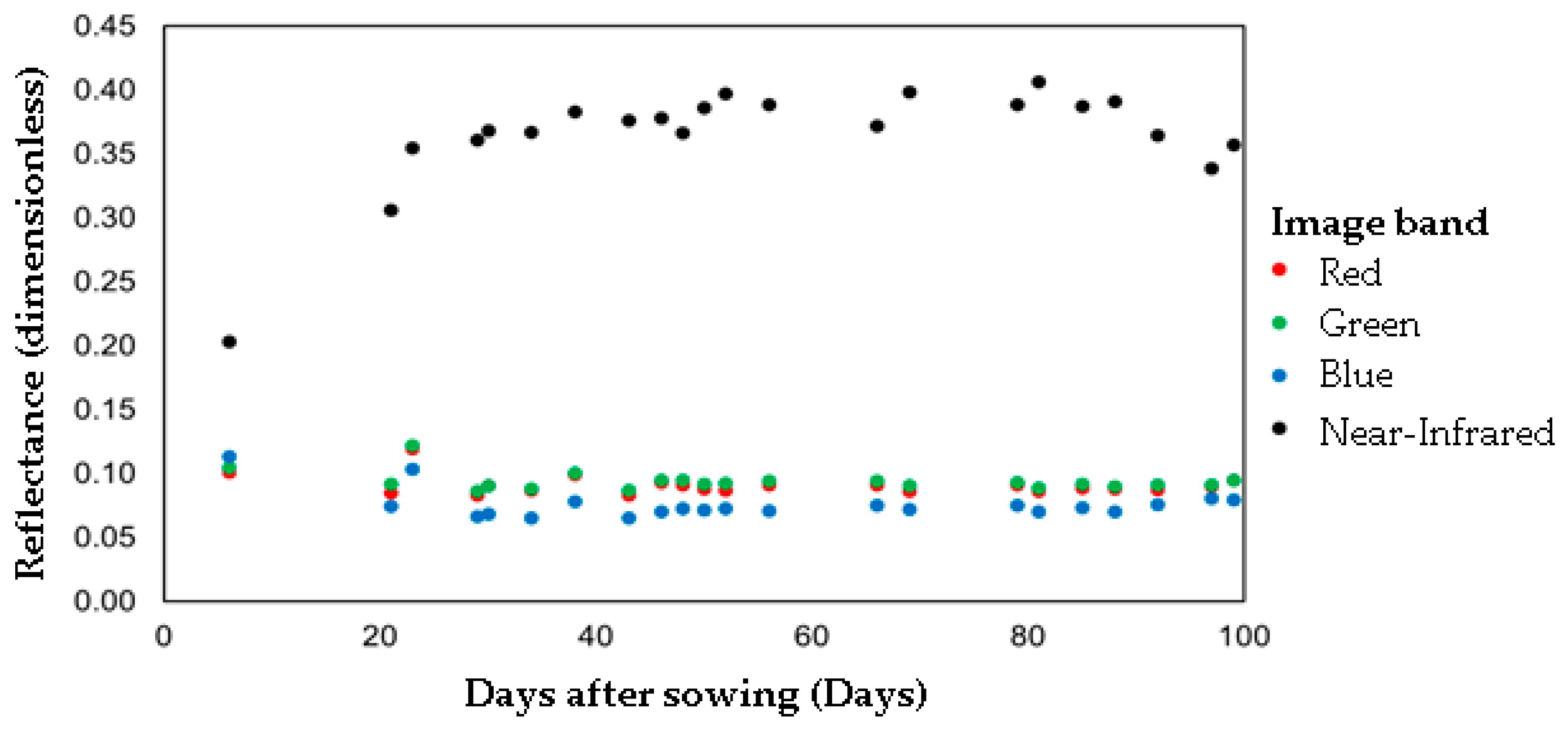
3.2. Satellite Imagery Data

A total of 22 satellite images that presented less than 1% of cloud cover over the area of study from 1 May and 31 August of 2017 were selected. A total of 88 spectral bands were obtained for the period of the crop cycle. The 88 spectral bands did not present a correlation with carrot yield values, despite the reflectance of the bands showing a relationship with the plant vegetative stage. This non-linear correlation highlights the suitability of applying RF to this dataset since it can cope with non-linear problems. The NIR band reflectance increased during the growing period and the reflectance values of R, G and B bands decreased at 40 days after sowing (DAS) (Figure 5). In this period, aerial parts (leaves) of the crop are in intense development stages [40,41,42]. At 40 DAS, the amplitude across R, G and B bands decreases in association with the highest growth phase of carrot roots [40,41,42]. Similar reflectance behavior was found for crops other than carrots, such as (a) tomato, (b) potato and (c) watermelon, when the NIR band has the highest reflection rate during the growth period [43].

As shown in Figure 5, despite the difficulties in obtaining satellite imagery during the carrot crop cycle caused by the rainy season, it was possible to gather images from almost all the stages leading up to harvest with minimal gaps (6–21 DAS, 57–65 DAS and 69–78 DAS). [44] emphasized the problem of obtaining satellite images during rainy seasons in predicting carrot and corn crop water footprints. Nevertheless, despite the absence of satellite images during the rainy season, it was possible to move forward with the RF regression model in this study to predict carrot yield by relying on spectral bands collected from satellite imagery data during the dry periods.

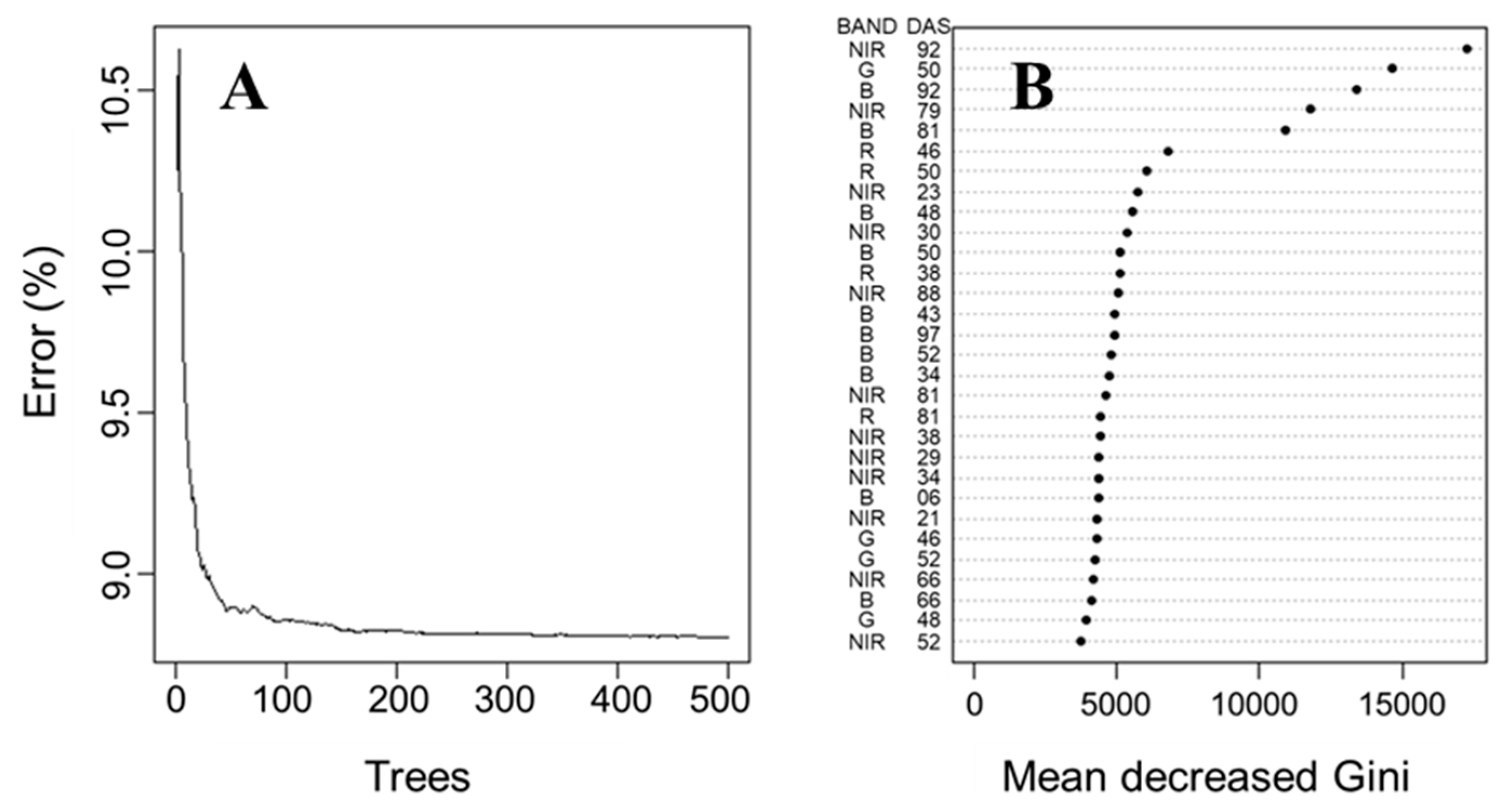
3.3. Random Forest Regression Prediction

The predictive precision curves shown in Figure 6 were constructed from the mean execution error values using actual and predicted carrot yield values generated by each reduced model. A mtry value equal to 29 (33% of the observations) was used, similar to the default value of the randomForest package. According to Bernard et al. [45], this default value of mtry is reasonable but can be improved upon. After adjustments of the mtry values, ntree values were changed from 0 to 500 with an increment of one tree at a time (Figure 6A). When the number of decision trees in RF increases, the error rate in each case decreases and gradually converges [46]. The average error rate of RF was close to 8.8% for both ntree values of 100 and 500. Therefore, a ntree value of 100 was chosen, as it was close to the minimum error rate, maximizing accuracy. This value corresponds with the elbow on the graph, a method used to select the best number of trees, similar to [47].

The five most important variables used to predict carrot yield with RF regression were identified as (a) NIR spectral band at 92 DAS, (b) NIR spectral band at 79 DAS, (c) green spectral band at 50 DAS, (d) blue spectral band at 92 DAS and (e) blue spectral band at 81 DAS (Figure 6B). The removal of important predictor variables in RF regression compromises the model’s accuracy, as it causes an increase in the mean decreased Gini values. On the other hand, the removal of uninformative or noisy predictor variables has little effect on accuracy [33,46,48], as mean decreased Gini values only fluctuate slightly (Figure 6B). Figure 6B shows that the RF regression model can accurately predict carrot yield with only five predictive variables instead of relying on the use of the 88 predictive variables. In addition to that, NIR and blue bands are the most present in the top 30 important variables used in the model. Thus, it suggests that carrot yield is more related to blue and NIR bands than red and green bands.

As shown in

Table 2. Random forest variables setting and evaluation metrics.

P a	Seed	Mtry b	Dataset	Number of Observations	Ntree c	RMSE d	R 2,e	MAE f
88	123	29	Training	9961	500	2.98	0.80	1.97
					100	2.97	0.80	1.96
			Test	5132	500	2.99	0.78	1.97
					100	2.99	0.78	1.97
			Entire	15093	500	2.64	0.82	1.74
					100	2.64	0.82	1.74

^a Total predictor variables; ^b number of variables tried at each split; ^c number of trees; ^d root mean squared error in Mg ha⁻¹ (Equation (2)); ^e coefficient of determination (Equation (3)); ^f mean absolute error in Mg ha⁻¹ (Equation (4)).

, R² values are equal for ntree values of 100 and 500, despite the datasets used (training and test). This result is expected since the error rate was close to the minimum value, as shown in Figure 6A. The training dataset is the only one that presents different absolute values of RMSE and MAE across ntree values. The evaluation metrics in Table 2 are the result of the RF regression model applied to datasets containing raw spectral data from satellite imagery, which differs from the common approach based on the application of VIs derived from spectral bands to monitor crops or predict yield in agriculture [18,19,20,21]. Most studies are conducted to predict crop yield relying on vegetation indices, for example, wheat [49,50,51] and corn crops [52,53,54,55].

In this study, the RF regression algorithm using only five temporal spectral bands presented an R², RMSE and MAE of 0.80, 2.97 Mg ha⁻¹ and 1.96 Mg ha⁻¹ for the training dataset for ntree equal to 100. The test dataset presented values of 0.78, 2.99 Mg ha⁻¹ and 1.97 Mg ha⁻¹ for R², RMSE and MAE, respectively. Furthermore, values of 0.82, 2.64 Mg ha⁻¹ and 1.74 Mg ha⁻¹ for R², RMSE and MAE, respectively were obtained using the entire dataset (Table 2).

Coefficient of determination values higher than 0.78 (Table 2) are not always found in studies that use VIs or spectral bands to forecast yield from crops in which the commercial product is grown below the ground, despite the use of statistical ML techniques. [19] predicted potato crop yield by applying linear regression models to the VIs database and reached R² values ranging from 0.39 to 0.65. [56] estimated peanut crop yield from a simple simulation model that included the use of leaf area index (LAI) and other variables, resulting in R² values of 0.30. [44] found a value of 0.67 for R² comparing observed and predicted yields from a linear model based on a soil-adjusted vegetation index (SAVI) obtained from Landsat-8 during the carrot growth period.

The evaluation metrics shown in Table 2 highlight the suitability of using RF regression on a database composed of raw spectral bands in predicting carrot yield, setting it apart from the common approach based on vegetation indices [49,50,51]. It is worth noting that the application of ML on a spectral band database instead of VIs corroborates the idea that ML applications are expected to find new patterns that provide insight and help speculate about occluded interactions in the field where there is a lack of prior knowledge and hypotheses [9].

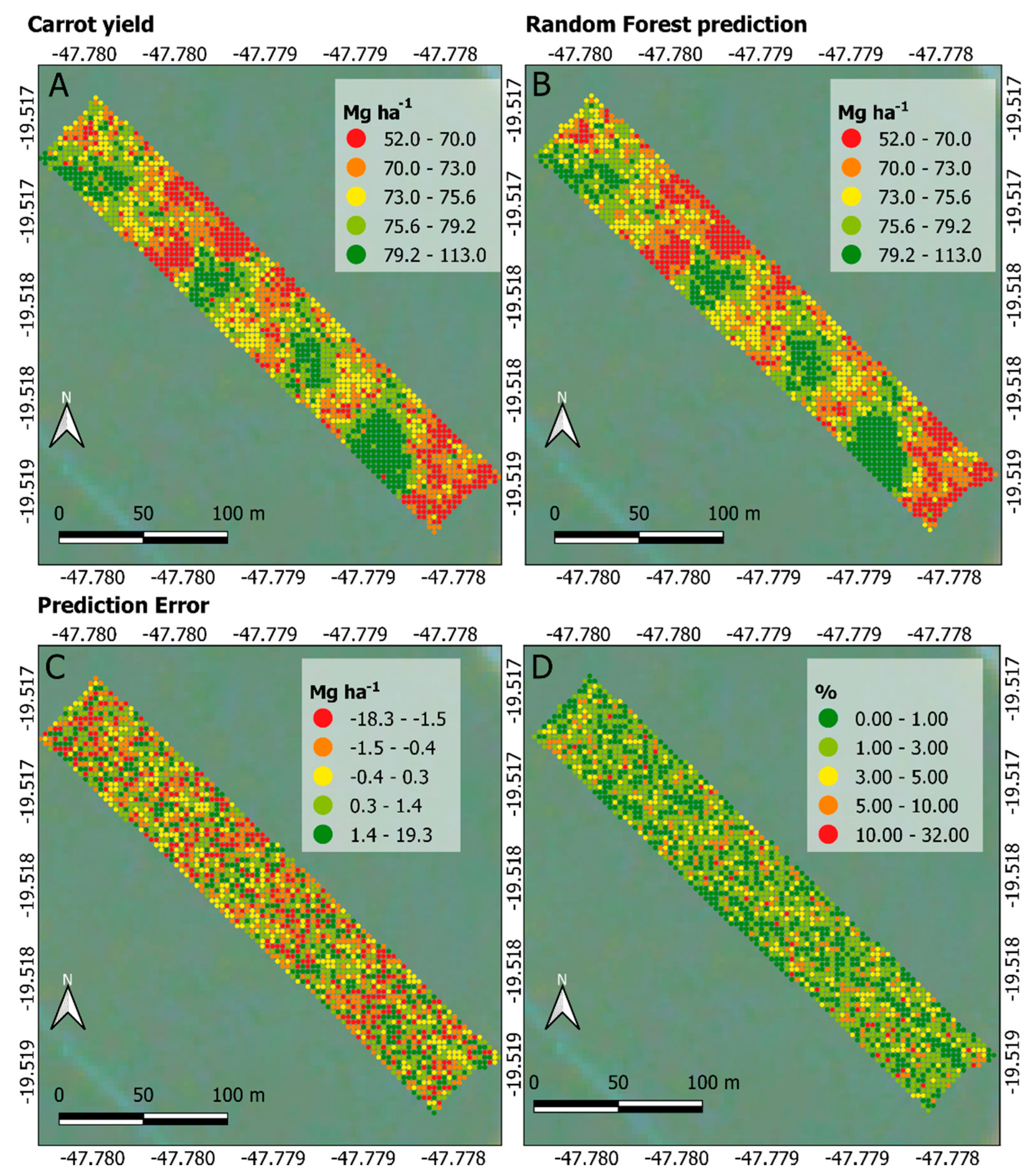
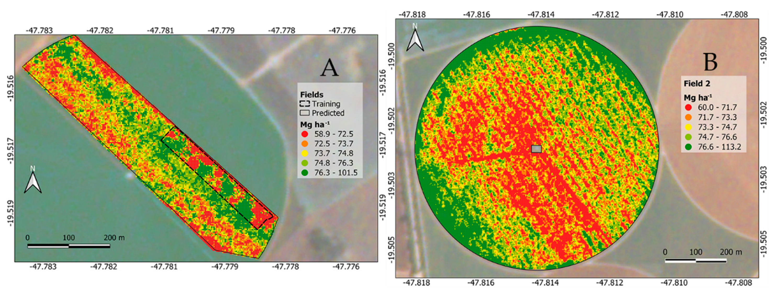
3.4. Carrot Yield Map Visualization

As shown in Figure 7A,B, the spatial yield patterns correspond to each other, highlighting the model’s goodness of fit for the entire dataset, which is to be expected based on the statistical metrics shown in Table 2. Figure 7C presents the error between predicted and observed yields, ranging from −18.3 to 19.3 Mg ha⁻¹ (35% variation, approximately). [44] found average error values of 4%, 14%, 18% and 38% between observed and predicted yield over four experimental carrot plots. In this study, the average yield error rate was about 0.3%, which again highlights the suitability of the RF regression model in predicting carrot yield. Figure 7D shows that errors below 5% prevail when looking at the punctual error rate between observed and predicted yield. Despite the lower error rate found in this study, it is not possible to make a fair comparison between percentage errors from this work and those in [44] because they presented only the observed carrot yield map and average results.

In this study, it was possible to use 22 high-resolution satellite images (88 spectral bands with 3 m × 3m spatial resolution) to feed into the RF regression algorithm, selecting the five most important predictors and then fitting a yield prediction model. This differs from [44], where 6–7 images with a lower spatial resolution (30 m × 30 m) were obtained during carrot crop development and fitted using linear regression to predict yield, using only SAVI values of one day, instead of fitting a multiple linear regression based on the temporal SAVI values, which could have yielded better results.

The focus in this paper was to generate an RF regression model to predict carrot yield based on satellite spectral bands and ground-truth yield samples, a goal which was successfully achieved, as seen on the metrics presented in Table 2 and visualized in Figure 7. The application of the generated model beyond the limits of the ground-truth yield samples is shown in Figure 8.

The prediction of carrot yield based on spectral bands and RF regression shows potential in its application, as ML can find new relations between variables [9]. This highlights the importance of using spectral bands instead of VIs to forecast yield, VIs being the result of the combination of spectral bands.

The patterns in Figure 6 are the same as highlighted in Figure 8A, indicating that the RF fitted model in this study is suitable for predicting carrot yield without the necessity of being compared to a ground-truth. The spatial variability of carrot yield in this field (Figure 8B) is useful in investigating the causes of root variability and can guide decisions to improve crop management [57].

The fusion of punctual yield sampling (ground-truth) data, remote sensing imagery data and application of a ML algorithm proved that carrot yield can be accurately estimated and mapped. Having a carrot yield map supports the application of PA techniques in understanding and identifying crop variability [58].

3.5. Future Perspectives

Future works should aim to evaluate the minimum area and number of ground-truth samples necessary to faithfully represent larger areas when applying the RF regression algorithm to predict crop yield based on temporal spectral data from satellite imagery, and not only for carrot crops. In addition to that, it is also necessary to evaluate the possibility of estimating carrot yield from satellite imagery with different spatial and temporal resolutions.

Hopefully, this approach of applying ML techniques to datasets containing a certain number of ground-truth samples in a given area and the temporal spectral data from the crop canopy cycle will allow the creation of accurate yield maps to help support decision makers in enhancing their crop production with respect to the PA goals.

4. Conclusions

The application of a random forest regression algorithm on a database composed of temporal spectral bands from high spatial resolution satellite imagery during carrot crop development and carrot yield punctual sampling (ground-truth) proved to be a suitable machine learning approach to forecast carrot yield in commercial fields. The RF regression model was successfully developed and implemented in predicting carrot yield based on raw temporal spectral bands with an error of 2.7 Mg ha⁻¹, achieving a coefficient of determination of 0.82 within one crop season. A carrot yield mapping tool was developed from a predictive model generated from a smaller area and then applied to larger areas that contained the same predictive variables.

References

1. Vega, A.; Córdoba, M.; Castro-Franco, M.; Balzarini, M. Protocol for automating error removal from yield maps. Precis. Agric. 2019, 20, 1030–1044. [Google Scholar] [CrossRef]
2. International Society of Precision Agriculture (ISPA). Available online: https://www.ispag.org (accessed on 24 March 2020).
3. Colaço, A.F.; Trevisan, R.G.; Karp, F.H.S.; Molin, J.P. Yield mapping methods for manually harvested crops. In Precision Agriculture’15; Stafford, J.V., Ed.; Wageningen Academic Publishers: Wageningen, The Netherlands, 2015; pp. 39–44. [Google Scholar]
4. Simbahan, G.C.; Dobermann, A.; Ping, J.L. Screening yield monitor data improves grain yield maps. Agron. J. 2004, 96, 1091–1102. [Google Scholar] [CrossRef]
5. Erkan, M.; Dogan, A. Harvesting of horticultural commodities. In Postharvest Technology of Perishable Horticultural Commodities; Yahia, E.M., Ed.; Woodhead Publishing: Cambridge, UK, 2019; pp. 129–159. [Google Scholar]
6. Fulton, J.; Hawkins, E.; Taylor, R.; Franzen, A. Yield Monitoring and Mapping. In Precision Agriculture Basics; Shannon, D.K., Clay, D.E., Kitchen, N.R., Eds.; ASA, CSSA, and SSSA: Madison, WI, USA, 2018; pp. 63–78. [Google Scholar]
7. Liu, J.; Li, J.; Li, W.; Wu, J. Rethinking big data: A review on the data quality and usage issues. ISPRS J. Photogramm. 2015, 115, 134–142. [Google Scholar] [CrossRef]
8. Wolfert, S.; Ge, L.; Verdouw, C.; Bogaardt, M.J. Big data in smart farming—A review. Agric. Syst. 2017, 153, 69–80. [Google Scholar] [CrossRef]
9. Hochachka, W.M.; Caruana, R.; Fink, D.; Munson, A.; Riedewald, D.; Sorokina, D.; Kelling, S. Data-mining discovery of pattern and process in ecological systems. J. Wildlife Manage. 2007, 71, 2427–2437. [Google Scholar] [CrossRef]
10. Chlingaryan, A.; Sukkarieh, S.; Whelan, B. Machine learning approaches for crop yield prediction and nitrogen status estimation in precision agriculture: A review. Comput. Electron. Agric. 2018, 151, 61–69. [Google Scholar] [CrossRef]
11. Li, G.; Wan, S.; Zhou, J.; Yang, Z.; Qin, P. Leaf chlorophyll fluorescence, hyperspectral reflectance, pigments content, malondialdehyde, and proline accumulation responses of castor bean (Ricinus communis L.) seedlings to salt stress levels. Ind. Crops Prod. 2010, 31, 13–19. [Google Scholar] [CrossRef]
12. Usha, K.; Singh, B. Potential applications of remote sensing in horticulture—A review. Sci. Hortic. 2013, 153, 71–83. [Google Scholar] [CrossRef]
13. Huang, Y.; Chen, Z.X.; Tao, Y.U.; Huang, X.Z.; Gu, X.F. Agricultural remote sensing big data: Management and applications. J. Integr. Agric. 2018, 17, 1915–1931. [Google Scholar] [CrossRef]
14. Shanahan, J.F.; Schepers, J.S.; Francis, D.D.; Varvel, G.E.; Wilhelm, W.W.; Tringe, J.S.; Schlemmer, M.R.; Major, D.J. Use of remote sensing imagery to estimate corn yield. Agron. J. 2001, 93, 583–589. [Google Scholar] [CrossRef] [Green Version]
15. Marino, S.; Aria, M.; Basso, B.; Leone, A.P.; Alvino, A. Use of soil and vegetation spectroradiometry to investigate crop water use efficiency of a drip-irrigated tomato. Eur. J. Agron. 2014, 59, 67–77. [Google Scholar] [CrossRef]
16. Kamilaris, A.; Prenafeta-boldú, F.X. Deep learning in agriculture: A survey. Comput. Electron. Agric. 2018, 147, 70–90. [Google Scholar] [CrossRef] [Green Version]
17. Farid, H.U.; Bakhsh, A.; Ahmad, N.; Ahmad, A.; Mahmood-Khan, Z. Delineating site-specific management zones for precision agriculture. J. Agric. Sci. 2016, 154, 273–286. [Google Scholar] [CrossRef]
18. Peralta, N.R.; Assefa, Y.; Du, J.; Barden, C.J.; Ciampitti, I.A. Mid-Season High-Resolution Satellite Imagery for Forecasting Site-Specific Corn Yield. Remote Sens. 2016, 8, 848. [Google Scholar] [CrossRef] [Green Version]
19. Al-Gaadi, K.A.; Hassaballa, A.A.; Tola, E.; Kayad, A.G.; Madugundu, R.; Alblewi, B.; Assiri, F. Prediction of potato crop yield using precision agriculture techniques. PLoS ONE 2016, 11, 9. [Google Scholar] [CrossRef]
20. Skakun, S.; Franch, B.; Vermote, E.; Roger, J.-C.; Justice, C.; Masek, J.; Murphy, E. Winter wheat yield assessment using Landsat 8 and Sentinel-2 data. In Proceedings of the IGARSS 2018—2018 IEEE International Geoscience and Remote Sensing Symposium, Valencia, Spain, 22–27 July 2018; pp. 5964–5967. [Google Scholar] [CrossRef]
21. Gaso, D.V.; Berger, A.G.; Ciganda, V.S. Predicting wheat grain yield and spatial variability at field scale using a simple regression or a crop model in conjunction with Landsat images. Comput. Electron. Agric. 2019, 159, 75–83. [Google Scholar] [CrossRef]
22. Fieuzal, R.; Bustillo, V.; Collado, D.; Dedieu, G. Estimation of Sunflower Yields at a Decametric Spatial Scale—A Statistical Approach Based on Multi-Temporal Satellite Images. Proceedings 2019, 18, 7. [Google Scholar] [CrossRef] [Green Version]
23. Everingham, Y.; Sexton, J.; Skocaj, D.; Inman-Bamber, G. Accurate prediction of sugarcane yield using a random forest algorithm. Agron. Sustain. Dev. 2016, 36, 27. [Google Scholar] [CrossRef] [Green Version]
24. Narasimhamurthy, V.; Kumar, P. Rice Crop Yield Forecasting Using Random Forest Algorithm. Int. J. Res. Appl. Sci. Eng. Technol. 2017, 5, 1220–1225. [Google Scholar] [CrossRef]
25. Ngie, A.; Ahmed, F. Estimation of Maize grain yield using multispectral satellite data sets (SPOT 5) and the random forest algorithm. S. Afr. J. Geomat. 2018, 7, 11–30. [Google Scholar] [CrossRef] [Green Version]
26. Molin, J.P.; Mascarin, L.S. Colheita de citros e obtenção de dados para mapeamento da produtividade. Eng. Agric. Jaboticabal 2007, 27, 259–266. (In Portuguese) [Google Scholar] [CrossRef]
27. Centro de Abastecimento do Estado de São Paulo (CEAGESP). Available online: http://www.ceagesp.gov.br/wp-content/uploads/2015/07/cenoura.pdf (accessed on 24 March 2020). (In Portuguese)
28. Spekken, M.; Anselmi, A.A.; Molin, J.P. A simple method for filtering spatial data. In Proceedings of the European Conference of Precision Agriculture, Lleida, Spain, 7–11 July 2013. [Google Scholar]
29. Planet. Daily Satellite Imagery and Insights. Available online: https://www.planet.com (accessed on 24 March 2020).
30. Planet Labs. Developer Resource Center. 2020. Available online: https://developers.planet.com/tutorials/convert-planetscope-imagery-from-radiance-to-reflectance/ (accessed on 5 May 2020).
31. R Core Team. R: A Language and Environment for Statistical Computing; R Foundation for Statistical Computing: Vienna, Austria, 2018. [Google Scholar]
32. Planet. Planet Imagery Product Specification: PlanetScope & RapidEye. 2016. Available online: https://www.planet.com/products/satellite-imagery/files/1610.06_Spec%20Sheet_Combined_Imagery_Product_Letter_ENGv1.pdf (accessed on 5 May 2020).
33. Breiman, L. Random Forests. Mach. Learn. 2001, 45, 5–32. [Google Scholar] [CrossRef] [Green Version]
34. Blanco, C.M.G.; Gomez, V.M.B.; Crespo, P.; Ließ, M. Spatial prediction of soil water retention in a Páramo landscape: Methodological insight into machine learning using random forest. Geoderma 2018, 316, 100–114. [Google Scholar] [CrossRef]
35. Liaw, A.; Wiener, M. Classification and regression by randomForest. R News 2002, 2, 18–22. [Google Scholar]
36. Hastie, T.; Tibshirani, R.; Friedman, J. Random Forests. In The Elements of Statistical Learning: Data Mining, Inference, and Prediction; Springer: Berlin, Germany, 2009; pp. 587–603. [Google Scholar]
37. Stumpf, A.; Kerle, N. Object-oriented mapping of landslides using random forests. Remote Sens. Environ. 2011, 115, 2564–2577. [Google Scholar] [CrossRef]
38. Rahmati, O.; Pourghasemi, H.R.; Melesse, A. Application of GIS based data driven random forest and maximum entropy models for groundwater potential mapping: A case study at Mehran Region, Iran. Catena 2016, 137, 360–372. [Google Scholar] [CrossRef]
39. Quantum Geographic Information System (QGIS). Available online: https://qgis.org/en/site/forusers/download.html (accessed on 24 March 2020).
40. Thompson, R. Some factors affecting carrot root shape and size. Euphytica 1969, 18, 277–285. [Google Scholar]
41. Sri Agung, I.G.A.M.; Blair, G.J. Effects of soil bulk density and water regime on carrot yield harvested at different growth stages. J. Hortic. Sci. Biotech. 1989, 64, 17–25. [Google Scholar] [CrossRef]
42. Dawuda, M.M.; Boateng, P.Y.; Hemeng, O.B.; Nyarko, G. Growth and yield response of carrot (Daucus carota L.) to different rates of soil amendments and spacing. J. Sci. Technol. 2011, 31, 11–22. [Google Scholar] [CrossRef]
43. Guermazi, E.; Bouaziz, M.; Zairi, M. Water irrigation management using remote sensing techniques: A case study in Central Tunisia. Environ. Earth Sci. 2016, 75, 202. [Google Scholar] [CrossRef]
44. Madugundu, R.; Al-Gaadi, K.A.; Tola, E.; Hassaballa, A.A.; Kayad, A.G. Utilization of Landsat-8 data for the estimation of carrot and maize crop water footprint under the arid climate of Saudi Arabia. PLoS ONE 2018, 13, 2. [Google Scholar] [CrossRef] [PubMed] [Green Version]
45. Bernard, S.; Heutte, L.; Adam, S. Influence of hyperparameters on random forest accuracy. In Multiple Classifier System; Benediktsson, J.A., Kittler, J., Roli, F., Eds.; Springer: Heilderberg, Germany, 2009; Volume 5519, pp. 171–180. [Google Scholar]
46. Xu, Z.; Lian, J.; Bin, L.; Hua, K.; Xu, K.; Chan, H.Y. 2019. Water Price Prediction for Increasing Market Efficiency Using Random Forest Regression: A Case Study in the Western United States. Water 2019, 11, 228. [Google Scholar] [CrossRef] [Green Version]
47. Tracy, T.; Fu, Y.; Roy, I.; Jonas, E.; Glendenning, P. Towards Machine Learning on the Automata Processor. In High Performance Computing; Kunkel, J., Balaji, P., Dongarra, J., Eds.; Springer: Cham, Switzerland, 2016; Volume 9697, pp. 200–218. [Google Scholar]
48. Fox, E.W.; Hill, R.A.; Leibowitz, S.G.; Olsen, A.R.; Thornbrugh, D.J.; Weber, M.H. Assessing the accuracy and stability of variable selection methods for random forest modeling in ecology. Environ. Monit. Assess. 2017, 189, 316. [Google Scholar] [CrossRef] [PubMed]
49. Bushong, J.T.; Mullock, J.L.; Miller, E.C.; Raun, W.R.; Klatt, A.R.; Arnall, D.B. Development of an in-season estimate of yield potential utilizing optical crop sensors and soil moisture data for winter wheat. Precis. Agric. 2016, 17, 451–469. [Google Scholar] [CrossRef]
50. Pantazi, X.E.; Moshou, D.; Alexandridis, T.; Whetton, R.L.; Mouzaen, A.M. Wheat yield prediction using machine learning and advanced sensing techniques. Comput. Electron. Agric. 2016, 121, 57–65. [Google Scholar] [CrossRef]
51. Sun, J.; Rutkoski, J.E.; Poland, J.A.; Crossa, J.; Jannink, J.; Sorrells, M.E. Multigrain, random regression, or simple repeatability model in high-throughput phenotyping data improve genomic prediction for wheat grain yield. Plant Genome 2017, 10, 1–12. [Google Scholar] [CrossRef] [Green Version]
52. Sharma, L.K.; Franzen, D.W. Use of corn height to improve the relationship between active optical sensor readings and yield estimates. Precis. Agric. 2014, 15, 331–345. [Google Scholar] [CrossRef]
53. Sharma, L.K.; Bu, H.; Denton, A.; Franzen, D.W. Active-optical sensors using RED NDVI compared to red edge NDVI for prediction of corn grain yield in North Dakota, USA. Sensors 2015, 15, 27832–27853. [Google Scholar] [CrossRef]
54. Maresma, A.; Ariza, M.; Martínez, E.; Lloveras, J.; Martínez-Casasnovas, J.A. Analysis of Vegetation Indices to determine nitrogen application and yield prediction in maize (Zea mays L.) from a standard UAV service. Remote Sens. 2016, 8, 973. [Google Scholar] [CrossRef] [Green Version]
55. Tagarakis, A.C.; Ketterings, Q.M. In-season estimation of corn yield potential using proximal sensing. Agron. J. 2017, 109, 1323–1330. [Google Scholar] [CrossRef] [Green Version]
56. Noorhosseini, S.A.; Soltani, A.; Ajamnoroozi, H. Simulating peanut (Arachis hypogaea L.) growth and yield with the use of the simple simulation model (SSM). Comput. Electron. Agric. 2018, 145, 63–75. [Google Scholar] [CrossRef]
57. Gong, A.; Yu, J.; He, Y.; Qiu, Z. Citrus yield estimation based on images processed by an Android mobile phone. Biosyst. Eng. 2013, 115, 162–170. [Google Scholar] [CrossRef]
58. Mulla, D.J.; Schepers, J.S. Key process and properties for site-specific soil and crop management. In The State of Site-specific Management for Agriculture; Pierce, F.J., Sadler, E.J., Eds.; ACSESS: Madison, WI, USA, 1997; pp. 1–18. [Google Scholar]
Figure 1. Pivot location of the study sites in Brazil.
Ai 01 00015 g001
Figure 2. Semi-mechanized carrot harvesting system. Carrot harvester (A). Deposition of the roots next to the harvester (B). Root selection and roots suitable (inside boxes) and not suitable (on the floor) for trading (C). Carrot box georeferencing procedure (D).
Ai 01 00015 g002
Figure 3. Procedure to generate a carrot yield map. Extract polygon grid from a PlanetScope image with 3 m × 3 m spatial resolution (A,B); carrot boxes inside each pixel of 3 m × 3 m (C). Count of the number of boxes inside each pixel of 3 m × 3 m (D).
Ai 01 00015 g003
Figure 4. Carrot yield prediction and mapping flowchart.
Ai 01 00015 g004
Figure 5. The reflectance of the Planet Scope image bands throughout the crop cycle.
Ai 01 00015 g005
Figure 6. Random forest tuning. Error rate vs. number of trees (A) and variable importance according to mean decrease Gini (B). BAND = spectral bands; NIR = near-infrared; G = green; B = blue; R = red; DAS = days after sowing.
Ai 01 00015 g006
Figure 7. Maps generated from the carrot yield dataset. Observed yield in Mg ha−1 (A), predicted yield in Mg ha−1 (B), yield error in Mg ha−1 (C) and yield error in percentage (D).
Ai 01 00015 g007
Figure 8. Estimated carrot yield (Mg ha−1). Carrot area with the ground-truth strip (A) and outer carrot field in a central pivot irrigated area (B).
Ai 01 00015 g008