Article

Sieve: An Ensemble Algorithm Using Global Consensus for Binary Classification

Department of Electrical and Computer Engineering, Florida International University, Miami, FL 33174, USA
*
Author to whom correspondence should be addressed.
AI 2020, 1(2), 242-262; https://doi.org/10.3390/ai1020016
Submission received: 20 April 2020 / Revised: 14 May 2020 / Accepted: 21 May 2020 / Published: 26 May 2020
(This article belongs to the Section AI Systems: Theory and Applications)

Abstract

:
In the field of machine learning, an ensemble approach is often utilized as an effective means of improving on the accuracy of multiple weak base classifiers. A concern associated with these ensemble algorithms is that they can suffer from the Curse of Conflict, where a classifier’s true prediction is negated by another classifier’s false prediction during the consensus period. Another concern of the ensemble technique is that it cannot effectively mitigate the problem of Imbalanced Classification, where an ensemble classifier usually presents a similar magnitude of bias to the same class as its imbalanced base classifiers. We proposed an improved ensemble algorithm called “Sieve” that overcomes the aforementioned shortcomings through the establishment of the novel concept of Global Consensus. The proposed Sieve ensemble approach was benchmarked against various ensemble classifiers, and was trained using different ensemble algorithms with the same base classifiers. The results demonstrate that better accuracy and stability was achieved.

1. Introduction

In complex machine learning problems involving multiple-base classifiers, a consensus result can be achieved using an ensemble approach which can improve the accuracy of intermediate results. This ability of combining intermediate results creates an ensemble algorithm, which have recently been the focus of ongoing research [1], according to various machine learning approaches applied to numerous domains employing classification [2], regression [3] and clustering [4,5,6]. When considering the structure of Multiple Classifier Systems (MCS), the majority of their configurations consist of three procedures: topology selection, base classifier generation and consensus [7]. In most cases, the topology and the base classifier procedures are combined to generate improved and independent base classifiers, where their results are aggregated through an ensemble to produce greater accurate results through a process of compensating each classifier’s results. A salient aspect of this approach is that every successful enhanced ensemble algorithm e.g., [8,9,10,11] has improved one or more of these three procedures. The main emphasize of applying an ensemble is to improve the effectiveness of the consensus to produce a more accurate result of the predicted label.
The objective of the consensus is to determine the label of a sample, based on multiple base classifier predictions. The current available consensus techniques target identifying and making the accurate base classifiers which dominate the consensus. However, these practical generated ensembles may not be improved as expected, due to the following five shortcomings: (1) Curse of Conflict (CoC), (2) uncertainty of accuracy improvement, (3) erratic magnitude of accuracy improvement, (4) Imbalanced Classification (IC) and (5) difficulty of base classifier selection.
The aforementioned five shortcomings are originally derived from the CoC and each one is associated with the previous one(s). The CoC occurs when correct classifier predictions are cancelled through wrong classifier predictions, which can be attributed to the conflict among the non-homologous predictions [12]. A consequence of the CoC is that the employed consensus technique will perform inconsistently across diverse datasets. This impacts the effectiveness of the consensus and introduces two concerns, as described in (2) and (3); that is, any base classifier accuracy improvement cannot be guaranteed and any improvement in the accuracy’s magnitude is erratic [13]. Due to the fact that each ensemble result is derived from the base results, the former would present a similar extent of bias towards the same class as the latter. Accordingly, the existing consensus methodologies cannot effectively mitigate the issue of “Imbalanced Classification” (IC) [14]. Moreover, the IC will lead to the selection of the base classifier results employed in the consensus to be relegated to the results with a minimum accuracy of 50% to reduce the ensemble generation error [15]. As a consequence, in obtaining each ensemble result at the cost of maintaining multiple base classifiers, predicting each sample multiple times and executing a complex compensation/consensus procedure will largely increase the actual time complexities.
In the literature, various intelligent consensus solutions have been proposed [16] to overcome these five shortcomings, but to date, the proposed solutions lack the ability to achieve an ensemble’s main goal, “a guaranteed and significant accuracy improvement”. In this paper, we propose a novel ensemble algorithm named “Sieve”, which uses a new methodology called Global Consensus (GC) to resolve the previously identified concerns with the current ensemble approaches embedded in the traditional consensus methods.

2. Motivation

Various consensus techniques such as (weighted) voting, bagging, Bayesian formalism, belief theory, Dempster–Shafer’s evidence theory [17,18,19] have been developed to mitigate the CoC. As the beginning of the MCS, the (weighted) voting tried to avoid a wrong ensemble result by simply aggregating multiple-base results. Then, the bagging made improvements through generating more independent base classifiers which were trained on varied subsets. Other, more advanced, techniques focused on improving the base classifier’s results. For example, the Bayesian, belief and Dempster–Shafer theories have been utilized to quantify the importance of the base classifiers for improving the ensemble accuracy. Moreover, the most recent works aimed at reducing the error rate of the base classifiers. For instance, Rotation-Based SVM [20] generated diverse base results using random feature selection and data transformation techniques, which could simultaneously enhance both the individual’s accuracy and diversity within the ensemble. Essentially, the main difference of the existing practices is the adopted criterion for quantifying the importance of the base classifiers. Furthermore, these algorithms focus mainly on improving the accuracy of the ensemble result through reducing the misclassification associated with each sample. These can be identified as Local Consensus (LC), where the consensus emphasis is on the individual sample. The LC approach inherently suffers from a structural deficiency that causes unavoidable CoC, since the base classifier predictions will inevitably be in conflict, producing undesirable results.
Although the LC suffers from unsolvable deficiencies, it is undeniable that the consensus approach is an effective methodology to improve the ensemble’s accuracy because it compensates for the weakness or imperfect performance of the base classifiers. For instance, in order to resolve the poor relevance feedback issue that results from using a Support Vector Machine (SVM) classifier in the content-based image retrieval problem, many researchers have proposed a comprehensive classifier (ABRS-SVM) which combines an asymmetric Bagging-based SVM (AB-SVM) and a Random Sub-Space SVM (RS-SVM). The BRS-SVM itself has been a successful research project and 17 industry patents [21] have been generated directly or indirectly.
Therefore, emphasis on improving the ability of the consensus approach to avoid these deficiencies has rendered a superior result. It should be noted that although the principle of ensemble is to obtain a better result by combining the results of multiple base classifiers, the LC is not the only form of consensus. Hence, to avoid the CoC resulting from the sample-scoped consensus, another approach is to classify each sample by only one of the base classifiers. Due to the lack of sample-scoped consensus, the accuracy of each sample would be lower. In order to maintain a high accuracy, the most accurate classifiers will be identified (by testing on a subset called ranking, please refer to the next section for details) and employed first to label the samples, so that the misclassifications can be minimized. More specifically, each classifier is only responsible for classifying a portion of the samples to avoid the CoC. As a result, the ensemble labels are composed of the labels assigned by each base classifier. Since the described approach to consensuses is upon the full dataset, it is called Global Consensus (GC). The main difference between the two approaches, the LC and the GC, is that in the GC the base classifiers are not working together to label each sample, but instead cooperatively to label all the samples. One potential concern might be that the GC’s accuracy could be reduced, but since the consensus is not executed on individual samples, the opposite effect can be achieved because the accuracy is greatly improved with the reduction in or complete elimination of the CoC.

3. Sieve: A Global Consensus Ensemble

3.1. Overall Methodology

The proposed Sieve ensemble algorithm is similar to other ensemble algorithms, that is, it requires the presence of several trained base classifiers to participate in a consensus. The difference is the way that the base classifiers are employed in forming an ordered classifier chain. As shown in Figure 1, the base classifiers are placed in an ordered chain. Starting with the first classifier, each classifier will label an exclusive portion of the samples (i.e., the white circles). This process continues until the last classifier in the chain has labeled its portion. The motivation of employing the base classifiers in this manner is two-fold. (1) As mentioned in the last section, since the CoC is an inevitable problem unless we abandon the sample-scoped consensus, labeling each sample using one base classifier is the only available approach of classification. (2) Furthermore, in order to reduce the error rate on each sample, each base classifier is allowed to proactively/freely select a portion of samples to classify based on its strength. As a result, each sample will be labeled by the base classifier with the highest confidence, hence producing high-level aggregated ensemble results.
It is important to recognize that there are always a few samples that would not be labeled by any classifier (i.e., the black circles), then these samples will be labeled using a non-classifier procedure. In the GC, the base classifiers compensate each other in labeling the samples that are not labeled by the other base classifiers, instead of cancelling out correct predictions with incorrect predictions from other base classifiers when using LC. In conclusion, the approach taken in Sieve requires the construction of a classifier chain, where the process is divided into three procedures composing the life cycle of the chain: creation, refinement and employment.

3.2. Creation of Classifier Chain

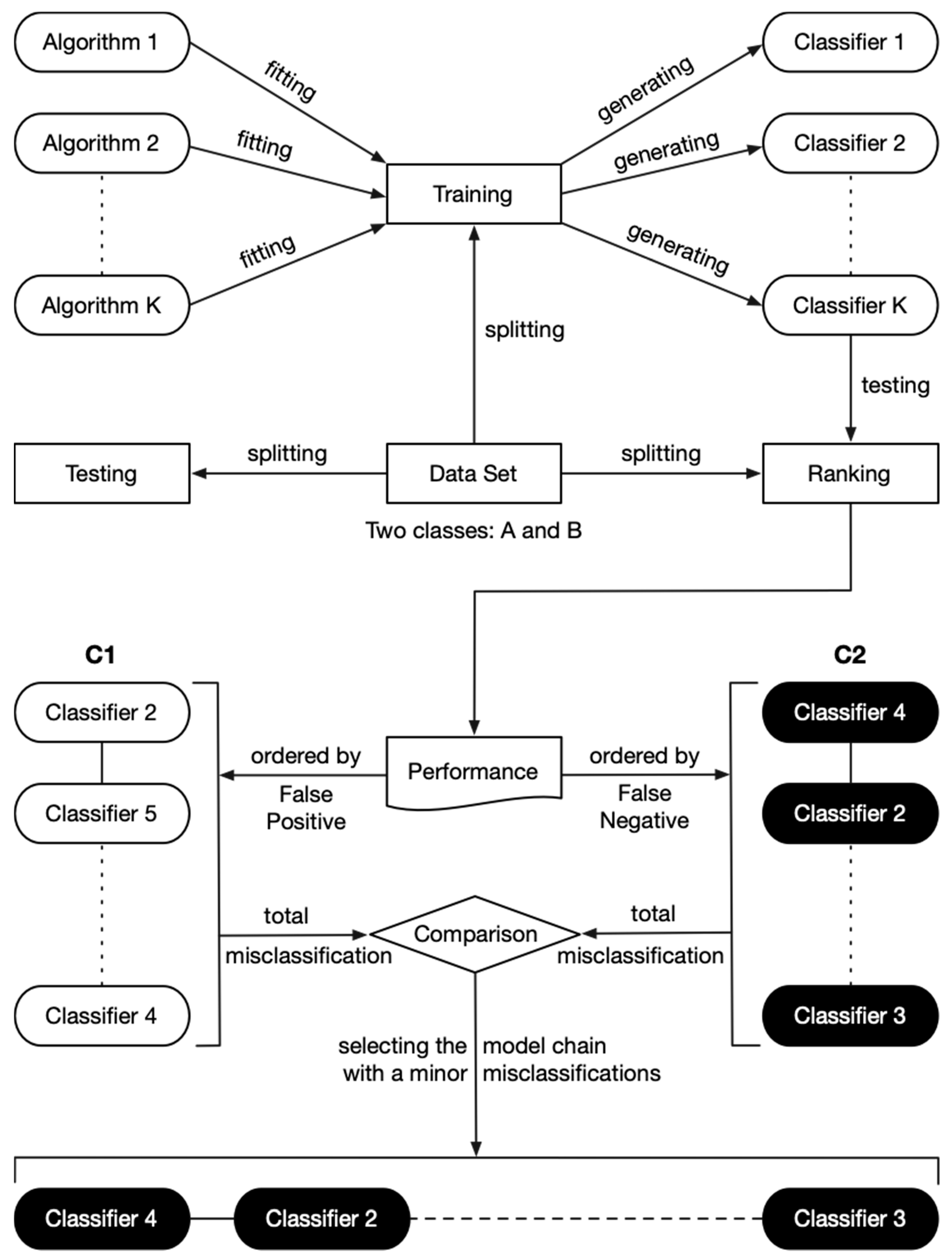
Referring to Figure 2, in order to train the base classifiers and create the classifier chain, the first step is to split the dataset into training, ranking and testing portions. The training portion is used to generate the base classifiers using different algorithms, where each algorithm from 1-K generates a corresponding classifier. The ranking portion is applied to evaluate each base classifier during the formation of the classifier chain. The testing portion of the dataset is used to evaluate the final classifier chain. Since both the latter two portions are used for evaluation, they should be about the same size and not less than 10,000 samples in general. These requirements should also be applied to the training portion. In addition, there is no special criterion in selecting the ranking portion of samples compared with the testing samples. In the case when a dataset consists of training and testing portions, the ranking portion would be extracted from the training portion. It is important to realize that the under-sampling of the ranking portion would result in an inaccurate classifier chain because the ensemble results are associated with the quality of classifier chain.
Once these different subsets of data are established, the process of training, ranking and testing can proceed. Firstly, the base classifiers will be generated by applying the training dataset, then the performance of each classifier is determined using the ranking dataset. This process evaluates and concludes the generalization capabilities of each base classifier. Next, using this information, all the base classifiers are sorted in ascending order according to false-positive (FP) and false-negative (FN), respectively (i.e., the best first). This will lead to the formation of two sorted classifier chains, the FP and FN sorted classifiers. Each chain contains all the base classifiers, but in different order. Finally, the total misclassifications associated with each of the two classifier chains are calculated, and we select the one with the least misclassification.
Assume K is five and there are two target classes, the A and the B, as in Figure 2. This leads to the training of five base classifiers 1–5, which are separately evaluated on the ranking dataset. Based on the outcomes, two sorted classifier chains are formed, C1: 2-5-1-3-4 for FP and C2: 4-2-1-5-3 for FN, in which higher score classifiers are positioned first in the chain (the order is not significant if the scores are the same). Here, FP represents misclassifying the class B as A, and FN represents misclassifying the class A as B, where C1 is ordered based on the misclassifications on the class B and C2 is ordered based on the misclassifications on the class A. Therefore, the misclassifications result from the two classifier chains indicates any inherent class bias with the base classifiers. Based on these results, the one with the lowest score will be selected as the base classifier chain, as it would result in less misclassification on a specific class. If C1’s misclassification score is higher than that of C2, then the C1 will be abandoned and C2 chain will be selected.
The motivation of utilizing the misclassification results as the basis for selecting a classifier chain is that, when invoking the base classifiers of C2 in the sequential of 4-2-1-5-3 to label the samples of class A, it will have a better accuracy in predicting the sample as class A. To illustrate the process, we apply a set of samples to the first base classifier, which is no.4 in C2, to make labeling predictions for all of the samples. The samples that were not labeled as class A will then be passed to the next base classifier, the no.2, in the chain, to continue the labeling process. This process will continue until the last base classifier, no.3, is employed. At this point, any remaining samples that most likely belong to the class B will be labeled to that class by a non-classifier procedure (refer to subsection “Employment of Classifier Chain”) to minimalize possible misclassification of them. Consequently, the ensemble result is the aggregation of the labels assigned by each base classifier, which will achieve high ensemble accuracy. A comprehensive explanation is presented in the subsection “Employment of Classifier Chain”. Two important points here: (1) the base classifiers are orderly invoked to only label a specific class; (2) the ensemble classification is a result of collaborations among all of the base classifiers and the last non-classifier procedure.

3.3. Refinement of Classifier Chain

The refinement of classifier chain is a process of identifying and eliminating the weak classifiers within the classifier chain. Although it may improve the ensemble accuracy, the main objective is to reduce the time complexity. Essentially, the refinement process is composed of a simplified classifier chain employment (refer to the next subsection) and a classifier elimination procedure.
Referring to Figure 3, assume that 10 samples in the ranking set are applied to the chain C2. Then each base classifier makes predictions on the unlabeled samples and will group some of them into class A by a base classifier, as expected. For example, the classifier no.4 predicts that among all the 10 samples, samples 3, 4, 7 belong to class A. Since the accuracy of this decision is higher than 50%, classifier no. 4 is retained. The remaining unlabeled seven samples are passed to the next classifier in the chain. From these seven remaining samples, classifier no.2 labels another four samples (i.e., samples 1, 5, 8, and 10) to the class A. Since the accuracy of this result is less than 50%, classifier no.2 is eliminated from the chain and the associated labeling result be cancelled. The number of unlabeled samples remains seven. Following this procedure, the base classifiers no.1 and no.3 are retained, as their accuracy is higher than 50%, and the base classifier no.5 is removed due to its lower than 50% accuracy. As a result, the base classifiers no. 4, 1, 3 are the only ones retained and the length of the refined classifier chain is reduced from five to three, a 60% reduction.
In the process of training each classifier, it is always important to address the issues of the overfitting problem. For Sieve, we need to point out that since the ranking process is involved in the forming of the classifier chain, this combination significantly mitigates the overfitting problem. In general, when using LC, there are two methods of splitting the training data to train the base classifiers, and none of them can effectively mitigate the overfitting problem. If the base classifiers are trained on the full training dataset, then the low independency among the base classifiers would lead to a stronger CoC. Training the base classifiers on varied subsets of the training dataset will make each base classifier lose the patterns in the excluded portion of the training set. It is critical to understand that the base classifiers in the LC-series compete among themselves, as each one wants to distinguish itself during the sample-scoped consensus. Therefore, this ability of the base classifiers would often be neutralized in such a competitive environment.
Now, as in the Sieve the training data are split into two groups, one for training the base classifiers and the another for determining the best combination of classifiers in the chain. Since the relationship among the base classifiers in GC-series is compensation, the formation of the classifier chain is a process of improving the mutual complementarity among them. The relationship among the generalization abilities of the base classifiers is always enhancing, hence resulting in a chain with a strong generalization ability. Most importantly, the complementarity is a property that is completely determined by the features of the base classifiers, instead of the training data, so the Sieve presents a stronger generalization ability than the LC-series ensemble algorithms on unseen data. At the end of this paper, a special experiment will be presented to highlight the primary reason that enables the Sieve approach to outperform the LC-series ensemble algorithms, emphasizing the significant structural advantages of employing GC.

3.4. Employment of Classifier Chain

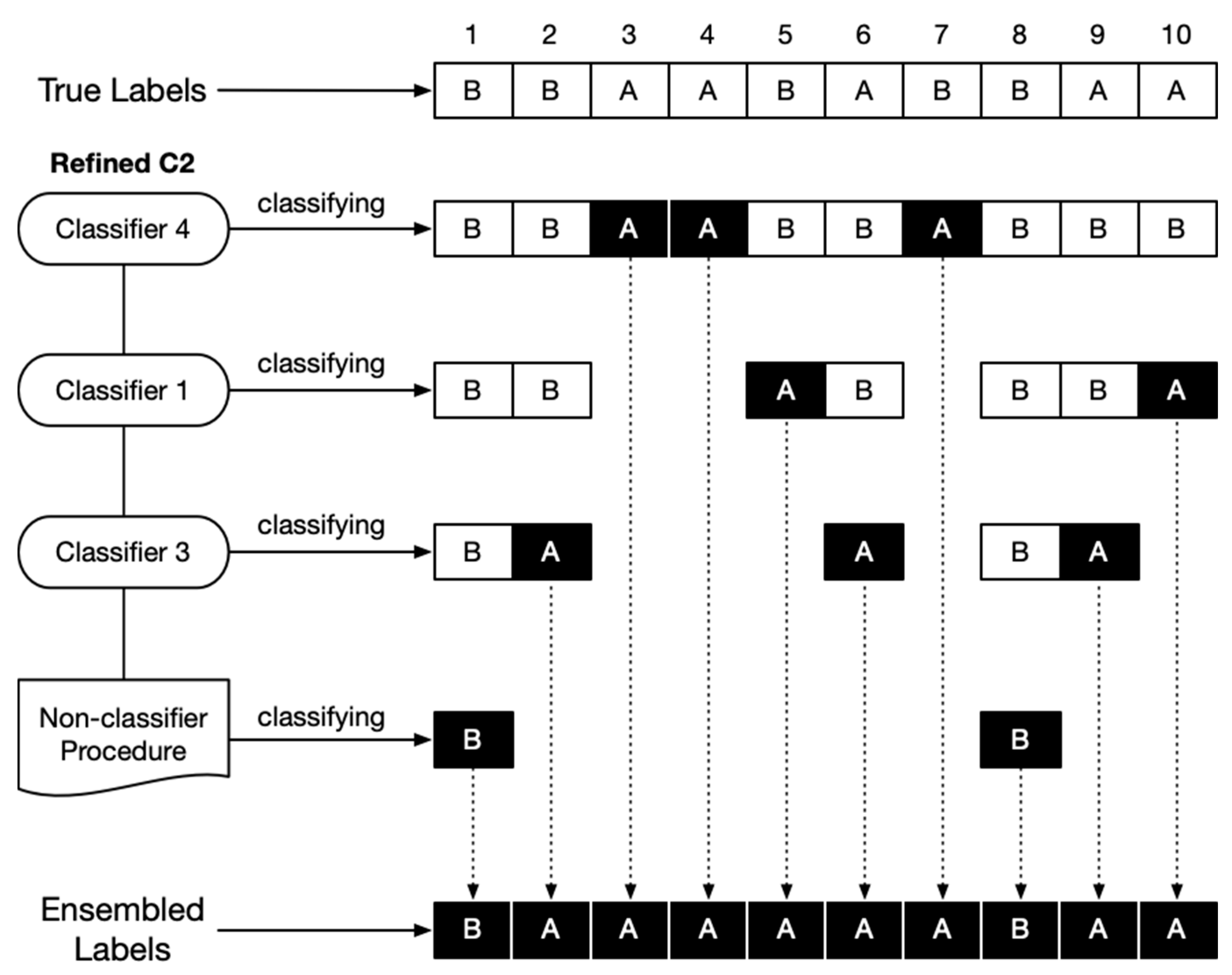
Employing the refined classifier chain on the testing set is the final procedure. Figure 4 illustrates the workflow of evaluating the refined classifier chain C2 on 10 samples. As a reminder, the C2 is ordered by the FN, which means its base classifiers no. 4, 1, 3, as a whole, are biased towards the class A, i.e., each base classifier is responsible for labeling a sample as class A if it predicts the sample in class A. In the figure, starting with the base classifier no.4, it makes predictions on all the 10 samples and label 3 samples (i.e., no.3, 4, 7) as class A. The remaining seven unlabeled samples are passed to the next base classifier, the base classifier no.1, which then makes prediction and labels samples no.5 and no.10 as class A. Now the remaining unlabeled samples are reduced to five, which are passed to the last base classifier, no.3. This classifier labels samples no.2, 6, and 9 as class A. The left-over samples no.1 and no.8 are not labeled and will be assigned to class B.
Overall, every sample will be either labeled to class A by one of the base classifiers or to the opposed group, class B. When a base classifier labels a sample, it is expected to have been done with high confidence because the classifier chain inherently has a bias to class A based on the evaluation results during the ranking process. In addition, high confidence is also associated with the non-labeled sample(s) in the class B. This is due to the fact that almost all the samples which truly belong to class A have been classified through the base classifiers, leaving most of the unlabeled samples to class B. Therefore, the Sieve technique maximizes the overall accuracy and reduces the misclassifications through the entire process. The proposed Sieve technique also incorporates a GC method as the new consensus approach which expands the consensus scope from each individual sample to all the samples in the dataset as a whole. A distinct difference between the LC and GC is that the former is built on a competitive ensemble idea which is susceptible to the CoC during the consensus, whereas the creation of GC is based on the compensation principle, which forms a robust ensemble classifier set through compensating the weaknesses among the base classifiers.

3.5. Pseudocode

The pseudocode of the Sieve is presented in Algorithm 1; please refer to the previous subsections for details.
Algorithm 1 Sieve
Input (2): the full-set of the dataset d a t f u l l , the collection of the K algorithms a l g K
Stand-alone Variable (4): the collection of the K base classifiers c l s b a s e K , the list of designated metric m of the base classifiers achieved on the dataset dat i n f d a t m , the selected/refined classifier chain C s e l / C r e f
Function (6) and Associated Variable (6): extracting n samples without replacement from d a t f u l l to form the subset d a t s u b = d a t f u l l . s p l i t ( n ) , employing the algorithm a l g on the dataset d a t to obtain a trained base classifier c l s b a s e = a l g . f i t ( d a t ) , employing a base classifier c l s b a s e / x or the non-classifier procedure p r o c n o n - c l s / x on the dataset d a t and returning the relevant information (e.g., the F P , the F N , the accuracy, the predicted samples s a m p p r e d , etc.) to i n f x = x . s c o r e ( d a t ) , forming a classifier chain C m e t r i c by sorting the K base classifiers in ascending order based on the designated metric m C m = c l s b a s e K . s o r t a s c ( i n f d a t m ) , summing up the designated metric m saved in i n f d a t m and returning the result s m = s u m ( i n f d a t m ) , updating the dataset d a t 1 by the difference with the dataset d a t 2   d a t 1 = d i f f ( d a t 1 , d a t 2 )
Output (2): the refined classifier chain C r e f and and varied performances P
Begin
1.  d a t t r a i n = d a t f u l l . s p l i t ( n 1 )
2.  d a t r a n k = d a t f u l l . s p l i t ( n 2 )
3.  d a t t e s t = d a t f u l l . s p l i t ( n 3 )
4. for each a l g a l g K do
5.    c l s b a s e = a l g . f i t ( d a t t r a i n ) ,
6.   recording c l s b a s e c l s b a s e K
7. for each c l s b a s e c l s b a s e K do
8.    i n f b a s e = c l s b a s e . s c o r e ( d a t r a n k )
9.   recording i n f b a s e i n f r a n k
10.  C F P = c l s b a s e K . s o r t a s c ( i n f r a n k F P )
11.  C F N = c l s b a s e K . s o r t a s c ( i n f r a n k F N )
12.  s F P = s u m ( i n f r a n k F P )
13.  s F N = s u m ( i n f r a n k F N )
14.  if s F P s F N then
15.    C s e l = C F P
16.  else
17.    C s e l = C F N
18.  c l e a r i n g   a l l   t h e   i n f o r m a t i o n   s a v e d   i n   i n f r a n k
19.  f o r   e a c h   c l s b a s e C s e l   d o
20.    i n f b a s e = c l s b a s e . s c o r e ( d a t r a n k )
21.    i f   i n f b a s e a c c u r a c y > 50 %   t h e n
22.       r e c o r d i n g   i n f b a s e i n f r a n k
23.       d a t r a n k = d i f f ( d a t r a n k ,   i n f r a n k s a m p p r e d )
24.    e l s e
25.       r e m o v i n g   c l s b a s e   f r o m   C s e l
26.  C r e f = C s e l
27.  f o r   e a c h   c l s b a s e C r e f   d o
28.    i n f b a s e = c l s b a s e . s c o r e ( d a t t e s t )
29.    r e c o r d i n g   i n f b a s e i n f t e s t
30.    d a t t e s t = d i f f ( d a t t e s t ,   i n f t e s t s a m p p r e d )
31.  i n f p r o c = p r o c n o n c l s . s c o r e ( d a t t e s t )
32.  r e c o r d i n g   i n f p r o c i n f t e s t
33.  c a l c u l a t i n g   P v a r i e d   b a s e d   o n   t h e   i n f o r m a t i o n   s a v e d   i n   i n f t e s t
End

3.6. Advantages

Except for the aforementioned strong generalization ability, the benefit of employing GC is that it overcomes those five shortcomings associated with the LC. (1) Since the consensus is no longer based upon each sample, which leads to the impact with the CoC (i.e., the conflict among the base predictions), that is instead completely eliminated. (2) As a consequence of the CoC elimination, there is an accuracy improvement that is manifested, since the ensemble accuracy must be at least as high as the first-invoked/most-accurate base classifier, even if all subsequent base classifiers misclassify all the unlabeled samples (i.e., the worst case). (3) In addition, the magnitude of the accuracy improvement is significant, since worst-case sample labeling would rarely occur in practice. (4) With respect to the mitigation of the IC, since the GC only utilizes the best partial ability of each base classifier (i.e., only labels one specific class) and assigns the left-over sample(s) to the opposite class, the bias on each cannot be fully transferred to/reflect on the Sieve. (5) Due to the fact that only the best partial ability will be utilized in the GC, one classifier is qualified to be the base classifier only if it can achieve a minimum accuracy of 50% toward either class instead of both classes. In that sense, the requirement of being a GC’s base classifier becomes lower compared with the LC, because achieving a decent accuracy on one class is the pre-requisite of achieving decent accuracies on two classes.
Regarding time complexity in terms of employment, it also has been significantly reduced after the base classifier chain is refined, because each base classifier in the chain is only responsible for making predictions on the samples that have not been previously labeled. For instance, consider a scenario that consists of a dataset of 10,000 samples that requires labeling and a chain that is composed of 10 base classifiers. If the LC is employed, then there are 100,000 (i.e., 10 × 10,000) predictions required, since each of the 10 base classifiers needs to predict all the 10,000 samples towards a consensus per sample. On the other hand, if the GC is adopted, the number of predictions is reduced to only 19,980 (i.e., 10,000 × (2 − (0.5) ^ 9)), under the conservative assumption that each base classifier will predict and label 50% of the samples remained.

4. Empirical Results: Six Experiments

4.1. Objectives and Methodologies

Six experiments carried out in this study can be divided into three groups based on their objectives. The first three experiments focus on the Sieve and LC-series ensemble algorithms employing the same group of base classifiers to compare their accuracy and stability. The objective of the next two experiments is to demonstrate the effectiveness of the classifier chain refinement process in its accuracy and length variations between the original and refined classifier chains. Finally, the last experiment is performed to reveal that the GC has a significant structural advantage over the LC. It is important to note that the goal is not to achieve the highest accuracy possible, but to show a better “accuracy improvement” compared with the LC-series algorithms when using the same base classifiers. Therefore, base classifiers are trained using the default configurations setup by Scikit-learn [22] and a dataset that has not been preprocessed to achieve consistency across these evaluations.
It is important to clarify that the stability (i.e., certainty of accuracy improvement) is a more important metric than the accuracy (i.e., the magnitude of accuracy improvement) in the evaluation of an ensemble classifier, because stability is the pre-requisite of the accuracy improvement. Therefore, only the accurate ensemble classifiers which have been validated in extensive experiments can truly reflect the performance of the existing practices. Accordingly, only 38 base classifiers and 20 LC-series ensemble classifiers trained by eight successful ensemble algorithms (i.e., Randomizable Filter [23], Bagging [24], AdaBoost [25], Random Forest [26], Random Sub-space [27], Majority Vote [28], Random Committee [29], and Extra Trees [30]) are involved in the first three experiments. Particularly, to maximize the accuracies of the compared ensemble classifiers (e.g., AdaBoost) which can only consensus upon the same type of base classifier; the most accurate base classifiers are employed as their base classifiers (refer to Table A1, Table A2, Table A3 and Table A4 in Appendix A). With respect to the evaluation data, a well-known benchmark dataset NSL-KDD [31], which includes two classes (i.e., Benign: B and Malicious: M) and two challenging test sets “test+” and “test-21” is employed to evaluate all the ensemble classifiers in terms of accuracy, precision, recall, F1-score and the Area Under the Receiver Operating Characteristic (AUROC). In addition, a dataset for Breast Cancer [32] is also evaluated by employing the same approach, which is a representative of small data. Since the refined classifier chains result from the big data (i.e., NSL-KDD) are much longer on than the small data (i.e., Breast Cancer), we will mainly interpreter/demonstrate the principles of the Sieve based on the results achieved on the first two experiments. Consequently, we place the results of the third experiment in Table A3, Table A4, Table A5 and Table A6 in Appendix A. The experiments will show the proposed algorithm can improve the performances on both the small and the big data.

4.2. Experiments 1, 2 and 3: Comparison of the Performances

We trained the 38 base classifiers on the dataset “KDDTrain+” (i.e., 125,937 samples). Table 1 and Table 2 show the performance of different ensemble techniques on the datasets, test-21 (i.e., 11,850 samples) and test+ (i.e., 22,544 samples), respectively. The rows above the third row from the bottom of the tables give the performance of the eight selected ensemble algorithms. More specifically, since five of the eight ensemble algorithms, denoted with asterisk, can produce multiple ensemble classifiers using varied base classifiers, we have to create multiple ensemble classifiers using these asterisk-marked algorithms to obtain a comprehensive result. Therefore, the performance of each of the algorithms with asterisk is averaged over the corresponding multiple ensemble base classifiers. For example, we built four AdaBoost ensemble classifiers by respectively employing four different base classifiers (i.e., algorithms), so in Table 1 and Table 2 the values under AdaBoost * are the average of the results from the four AdaBoost ensemble classifiers. As a result, the eight ensemble algorithms, with different ensemble classifiers and their corresponding performances are shown in Table A1 and Table A2 in Appendix A. Then, the second and the third rows from the bottom of Table 1 and Table 2 are the averaged performance of the 38 base classifiers and the eight selected LC-series ensemble algorithms, respectively. Observe that the averaged accuracy of the 38 base classifiers is lower than the majority vote, this is due to the fact that the majority vote only ensembles the best four base classifiers for its performance. Finally, the last row in the same tables is the performance of the Sieve technique.
Overall, these two tables show that the Sieve significantly outperforms the 38 base classifiers and the eight LC-series ensemble algorithms. For example, the accuracy of the Sieve has been improved by 31.75% (i.e., 85.43% − 53.68%) and 16.34% (i.e., 90.29% − 73.95%) compared with the base classifiers and by 28.99% (i.e., 85.43% − 56.44%) and 14.40% (i.e., 90.29% − 75.89%) compared with the LC-series ensemble classifiers. Most importantly, the Sieve is able to resolve or at least largely mitigate the IC. For instance, due to the fact that the differences between the precision(M) and precision(B) of the base classifiers are 66.16% (i.e., 91.46% − 25.30%) and 29.71% (i.e., 93.25% − 63.54%), separately, it indicates that the base classifiers are seriously biased towards the class M in both experiments. However, the Sieve is able to reduce the corresponding differences to 33.97% (i.e., 92.55% − 58.58%) and 4.44% (i.e., 92.25% − 87.81%). By contrast, the LC-series ensemble classifiers still result in high differences of 61.68% (i.e., 87.61% − 25.93%) and 26.81% (i.e., 92.25% − 65.44%) on the same metrics. If the averaged reduction rates of the precision difference are used to evaluate the ability to calibrate the bias base classifiers (i.e., scale of 1), the Sieve and the LC-series ensemble classifiers are scored at 0.6686 (i.e., 66.86% = [(66.16% − 33.97%)/66.16% + (29.71% − 4.44%)/29.71%]/2) and 0.0827 (i.e., 8.27% = [(66.16% − 61.68%)/66.16% + (29.71% − 26.81%)/29.71%]/2), respectively. Accordingly, we can consider that the Sieve is 8.08 (i.e., 0.6686/0.0827) times stronger than the LC-series ensemble classifiers in terms of handling the IC problem.
On the other hand, since the data pattern of the test-21 and test+ are somewhat varied, it is inevitable that all the classifiers will generate different results based on these two test sets. However, when the same ensemble classifier performs very differently on the two test sets, it indicates that this classifier would be more vulnerable/sensitive to the pattern variations (i.e., unstable performance). According to the results of the experiments, the difference in accuracy when the LC-series ensemble classifiers were applied to these two test datasets can reach a value of 20% (i.e., 75.89% − 56.44%), whereas the same metric is only 4.86% (i.e., 90.29% − 85.43%) for the Sieve. This comparison indicates that the Sieve would be 4.12 (i.e., 20/4.86) times more stable on the unseen data/diversity patterns, which means that the Sieve has a much broader range of practical applications. In addition, since the difference in the accuracy of the base classifiers for the same two datasets is also about 20% (i.e., 73.95% − 53.68%), it indicates that the erratic accuracy achieved with the LC-series ensemble classifiers is actually derived from the base classifiers. Therefore, the Sieve is able to greatly mitigate the inherent instabilities that are associated with the base classifiers. The final assessment is that the Sieve’s advantage in accuracy and stability is attributed to the structural advantage of the GC.
Similar conclusions can also be found in the evaluation results of the Breast Cancer; please refer to Table A3, Table A4 and Table A5 in Appendix A for details. It is worth mentioning that the LC-series ensemble algorithms are not able to improve the accuracy of the base classifier when the number of training samples is limited (i.e., 210), whereas, the Sieve can still improve the accuracy even though the number of training samples is only 50% of the LC-series (i.e., 105).

4.3. Experiments 3 and 4: Verifying the Effectiveness of the Classifier Chain Refinement

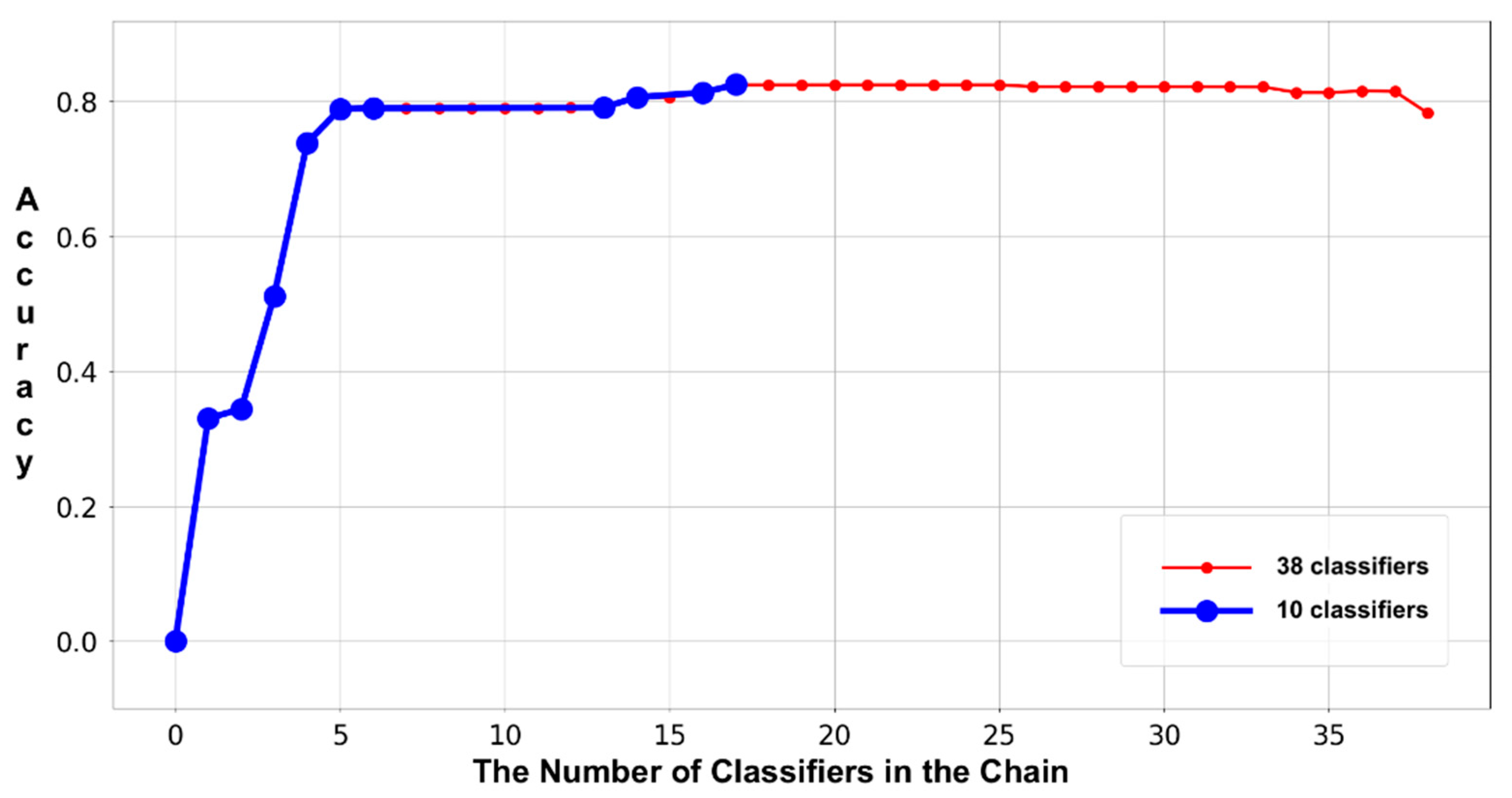
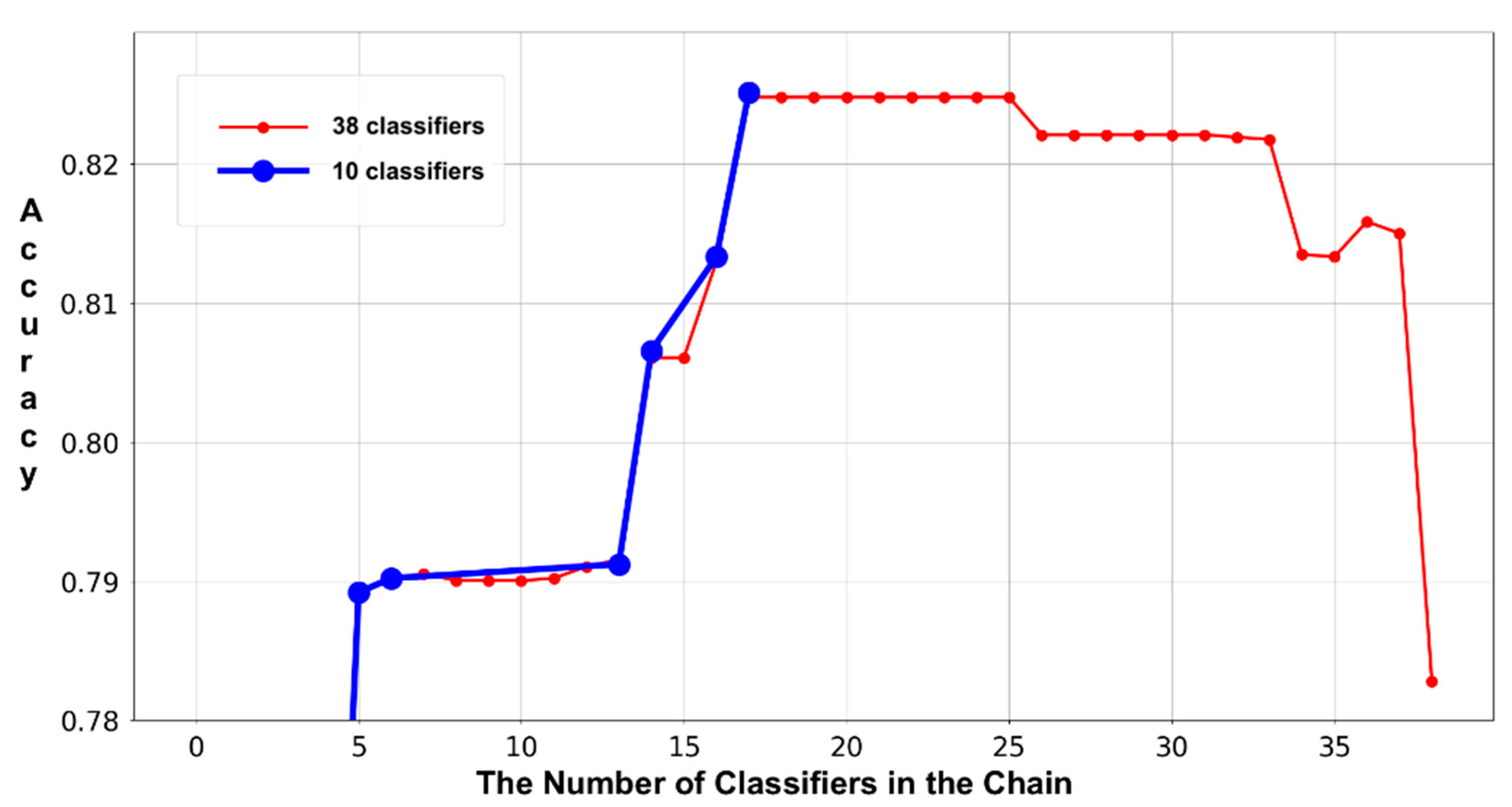
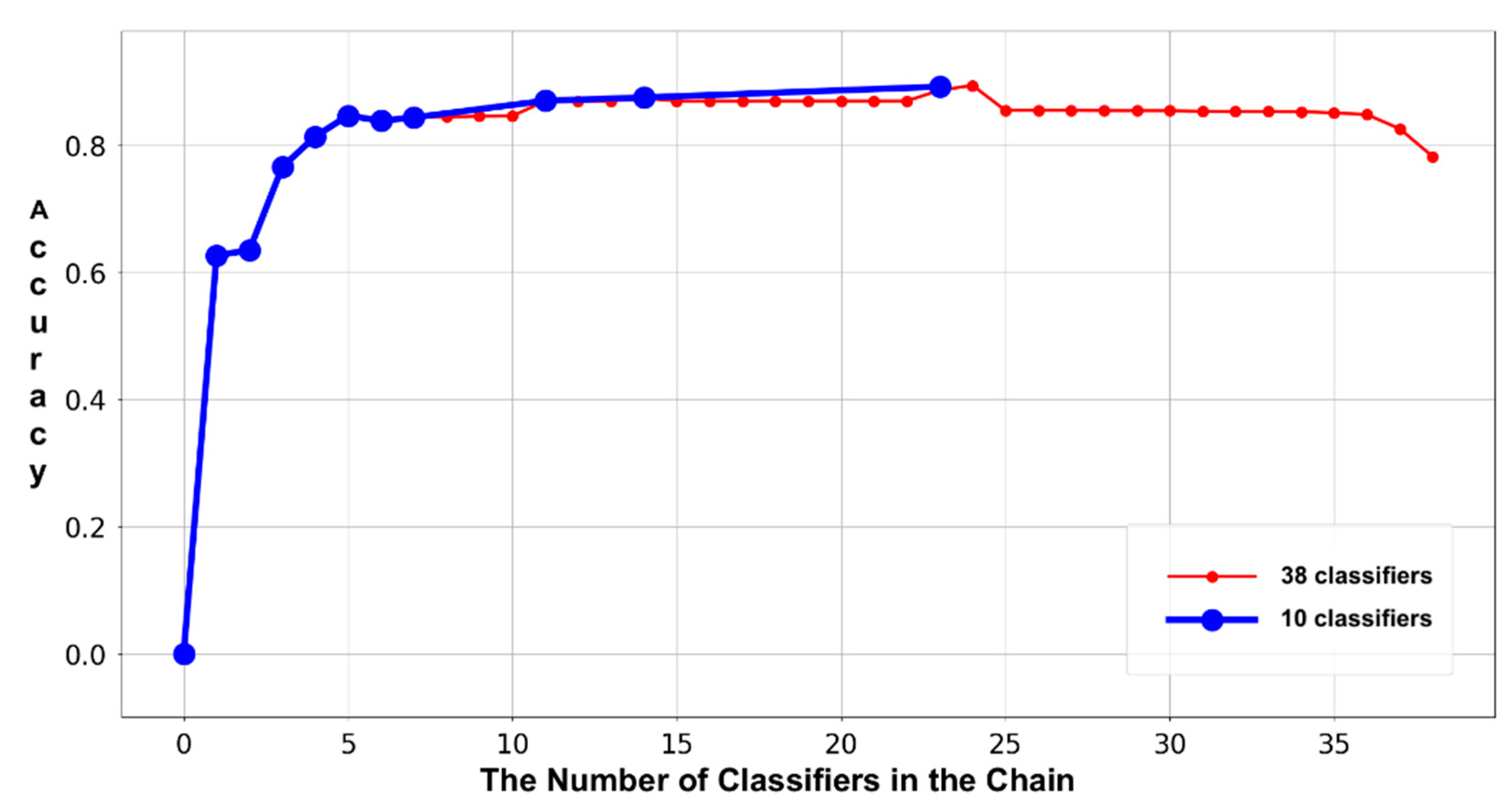
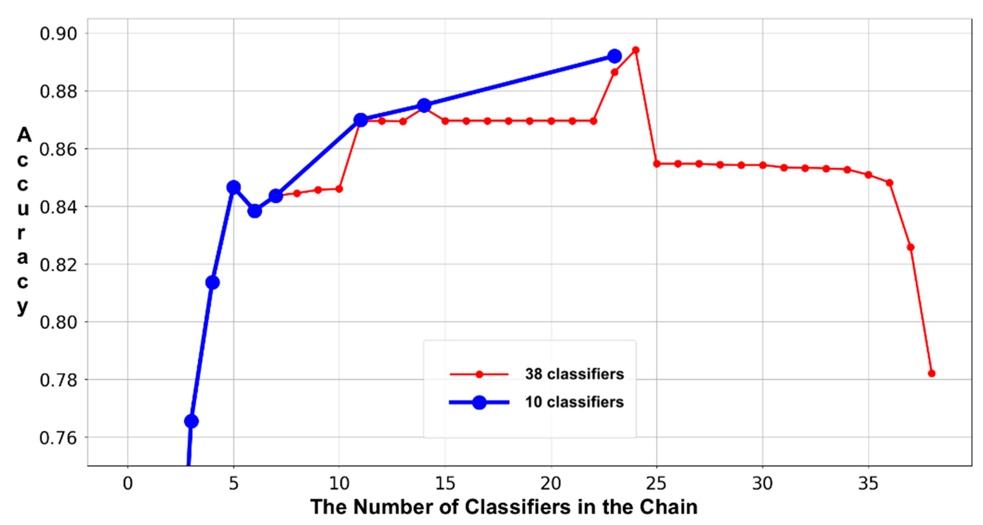
To verify the effectiveness of the refinement in the classifier chain, experiments 3 and 4 are performed to evaluate the variations in the accuracies and lengths of both the original and refined classifier chains on the two test sets. These two experiments record the accumulated accuracies of the invoked base classifier and form trajectories accordingly. As shown in the Figure 5, Figure 6, Figure 7 and Figure 8, the thin and thick lines are the trajectories that result from the original and refined classifier chains, separately. More specifically, each point represents the ratio between the number of correct-labeled samples and the number of all the samples in the dataset. Using the following example to demonstrate the method of calculating each accumulated accuracy point, assume there are 10 samples in the dataset; the first and last five samples belong to classes X and Y, respectively. Suppose also that the classifier chain that is biased towards class X includes two base classifiers: c1 and c2. If the c1 labels samples no.3–7 as class X, then all the rest of the samples are labeled as class Y. Then, the number of correct labels is six, which are samples no.3–5 (i.e., class X) and no.8–10 (i.e., class y). Therefore, the first accumulated accuracy point is 0.6 (i.e., 6/10). We have to emphasize that we are calculating every accuracy point by strictly executing the workflow of classifier chain employment. This means that we are simulating the workflow of employing a classifier chain with only one base classifier (i.e., c1) in the previous example. Since there are two base classifiers in the chain, adopting the same method, we need to clear all the labels that were not assigned by the c1 before calculating the second accumulated accuracy point, because the last base classifier c2 was not invoked. Accordingly, there are five samples (i.e., no.1, 2 and 8–10) passed to the c2. If the c2 labels samples no.1, 2, 10 as class X, then all the rest, samples no. 8 and 9, are labeled as class Y. Thus, the number of accumulated correct labels is 7: 3 labels (i.e., no.3–5, class X) result from the c1, 2 labels (i.e., no.1 and 2, class X) result from the c2 and the other two labels (i.e., no.8 and 9, the class Y) result from the last non-classifier procedure. Consequently, the second accumulated accuracy point is 0.7 (i.e., 7/10). In addition, we must distinguish the difference between calculating the accumulated accuracy and the accuracy that is used to eliminate the base classifiers. Referring to subsection “The Refinement of Classifier Chain,” a base classifier will be removed from the chain only when its accuracy is lower than 50%. In the previous example, the accuracy of the c2 for determining elimination is 0.67 instead of the accumulated accuracy 0.7, because it correctly labels the samples no.1, 2 and wrongly labels the sample no.10. In conclusion, the Sieve takes the accuracy that directly results from a base classifier into consideration when considering elimination and adopts the accumulated accuracy to verify the effectiveness of the classifier chain refinement. Referring to the figures, the accumulated accuracy might be increased, decreased or maintained, along with each new base classifier involved. Since the number of accumulated correct labels result from the newly involved base classifier, all the previous base classifiers and the last non-classifier procedure, it would be increased or decreased at some extents. There are also some points that maintain the accumulated accuracies, because the corresponding base classifiers do not label any new sample. The reason for this phenomenon is that all of their target samples have been labeled by the previous base classifiers, which means that their target samples are completely overlapping their predecessors. It is easy to understand that all the base classifiers that not improve the accumulated accuracies should be removed from the classifier chain and our classifier chain refinement successfully achieved this goal. The figures clearly indicate that the accuracy of each refined classifier chain (i.e., the last point on the thick lines) is roughly the same as that of the original classifier chain (i.e., the last point on the thin lines), which shows that the chain refinement procedure will not reduce the performance on accuracy.
In addition, the experiment data show that the low-ranked base classifiers are more vulnerable to being eliminated. This phenomenon is caused by two factors: the difference in accuracy and the overlap in terms of target samples between the high- and low-ranked base classifiers. For instance, there are 10 samples (i.e., including two classes, X and Y) and two base classifiers (i.e., c1 and c3, with the same accuracies of 60% in predicting the class X samples). In addition, let us make the following assumptions for the c1 and c3. If we invoke the c1 to label the 10 samples, it will label samples no.1–5 as the class X and the first three predictions (i.e., no.1–3) are correct. If we invoke the c3 to make predictions on the 10 samples, it will label samples no. 4–8 as the class X and the first three labels (i.e., no. 4–6) are correct. Under this assumption, if we form a classifier chain with the two base classifiers (i.e., the c1 in the first place) to label the 10 samples, the second-placed c3 will only label samples no.6–8 as the class X because samples no.1–5 have been labeled by the c1. Since the c3 (i.e., the low-ranked base classifier) can only make a correct prediction on sample no.6, its accuracy is only 33% and should be eliminated from the chain according to the chain refinement procedure. Furthermore, if there is another base classifier c2 between c1 and c3, and c2 has labeled sample no.6 as class X before invoking the c3, then the c3 will only label samples no.7, 8, hence reducing its accuracy to zero (i.e., more vulnerable to being eliminated). Although the exact assumed situation might rarely happen in practice, it is inevitable in reality, because any first-invoked base classifier would label (more or less) some samples that can be correctly labeled by its successors. Essentially, the magnitude of such affection (in terms of elimination) resulting from the high-ranked base classifiers toward a low-ranked base classifier is unpredictable, but the tendency is generally determined. Therefore, the aforementioned example is trying to explain a common phenomenon that a low-ranked base classifier is more vulnerable to being eliminated due to its low accuracy as well as the overlapping magnitude of the target samples between it and the predecessors. As a result, only the first several and a few middle base classifiers are retained in the classifier chain. The reduction rates in the two original classifier chains are 73.68% (i.e., (38 − 10)/38) in the first two experiments. Particularly, the reduction rate of the third experiment achieves 94.74% (i.e., 2/38; please refer to Table A5 in Appendix A). A possible reason for the difference in the reduction rates is that the small/big data would be more likely to be labeled/covered by a fewer/more base classifiers, so the length of the refined classifier chain would be proportion to the data size. However, this is only a trend instead of a definite conclusion because the reduction rate is determined by the base classifiers, and hence out of the control of the Sieve. As a result, the three experiments verify that the classifier chain refinement can effectively shorten the classifier chain without impacting the accuracy.
Moreover, the percentage of samples labeled by each base classifier/layer and the corresponding accuracy are shown in Table 3, where the two columns “Labeling Percentage” are computed via dividing the number of labeled samples (i.e., by the current layer) by the total number of samples; the two columns “Accuracy” represent the accuracy achieved by the current layer. For example, assume the total number of samples is 10. If the first base classifier labels four of 10 samples and three of the four labeled samples are correct, the percentage and the accuracy of this base classifier are 40% (i.e., 4/10) and 75% (i.e., 3/4), respectively. As a result, we can observe that the percentages and accuracies are (roughly) becoming smaller as more base classifiers are invoked. However, this is also a trend instead of a definite conclusion because there are some data that violate this pattern. For instance, the two labeling percentages of the base classifier no.3 are higher than the base classifier no.2. The two accuracies of the base classifier no.8 are higher than the base classifier no.7. A similar pattern can also be found on the layer-based performances result from the Breast Cancer; please refer to Table A6 in Appendix A for details.

4.4. Revealing the Significant Structural Advantage on the Global Consensus

Essentially, there are only three differences between the Sieve and the LC-series ensemble algorithms. These are: (1) utilizing the capabilities of every base classifier fully (i.e., labeling both classes) or partially (i.e., only labeling one class); (2) employing the base classifiers with or without a certain order (i.e., invoking based on the ranking or not); (3) labeling each sample via a consensus approach (i.e., combining multiple base predictions) or not. Therefore, the performance on accuracy between these two algorithms must be linked to one or more of these three points. In order to identify the actual reason, multiple hybrid ensemble classifiers are created and each one of them is a mixture of the Sieve and the LC-series ensemble algorithms. With respect to the approach of making prediction, each hybrid classifier performs in the similar way to the Sieve, i.e., the base classifiers are orderly invoked based on the ranking, and each base classifier adds one more vote of a specific class (instead of direct labeling) to a sample, but only when it predicts the sample as that class. From the respective of labeling, each hybrid classifier performs in exactly the same way as a LC-series ensemble classifier that adopts the majority vote as the consensus approach. A sample will be labeled as a specific class if the votes of that class are more than a half of the number of the base classifiers, otherwise, it will be labeled as the other class. It should be noted that each hybrid classifier is actually a special Sieve with a LC procedure.
The created hybrid ensemble classifiers are evaluated on the datasets test-21 and test+. Referring to Table 4 and Table 5, the performance between the Sieve and the hybrid ensemble classifiers is considerably different. Particularly, the accuracy of each hybrid ensemble classifier is even worse than that of the corresponding traditional LC-series ensemble classifier, despite the fact that it can orderly invoke the base classifiers similar to the Sieve. Due to the fact that the only difference between the hybrid classifiers and the Sieve is the involvement of an LC procedure, it can be concluded that this LC is the only possible reason that would cause the reduction in accuracy. Therefore, the reason that the Sieve greatly outperforms the LC-series ensemble classifiers can be attributed to the structural advantage that comes with the GC.

5. Conclusions

We have proposed a new ensemble algorithm, the Sieve, which outperforms existing ones on both the big and the small data by eliminating the problem of CoC, associated with the base classifiers in LC. This algorithm also skillfully handles the inherent bias associated with each classifier by constructing a classifier chain. The successful elimination of the problem of CoC is attributed to the GC, in which consensuses come from all of the samples as a whole instead of from each individual sample. (refer to subsection “Employment of Classifier Chain”) Consequently, the Sieve makes improvements on both accuracy (i.e., improved by 19.51% on average) and stability (refer to the subsection “Advantages”) by minimizing misclassifications in each procedure. In addition, it can effectively mitigate the IC by applying a non-classifier procedure to the classification process, which calibrates the biased ensemble results by labeling the leftover nonlabelled samples to the opposite group. Since the Sieve has to spend additional time constructing and refining the classifier chain, these manipulations will improve the time complexity in terms of the pre-processing.
The current version of the Sieve is only making improvements to the consensus procedure. The ensemble results could be further improved using other methods in the future. One of the methods is to train the base classifiers by various data subsets to enhance the independency among the base classifiers to benefit the overall accuracy of the entire classifier chain. Another promising method is to replace the non-classifier procedure by the base classifier with the lowest FN/FP if the refined classifier chain is ranked based on the FP/FN. Consequently, the number of misclassifications in the last layer would be reduced, improving the overall accuracy.
The current version that works for the binary classification can also be applied to resolve multi-class problems. Assume a dataset with three labels: A, B, C. We can create a binary dataset by re-labeling all samples that belong to class B or C as BC. Using this approach, three binary datasets can be created by combining every two classes alternately (i.e., AB, BC and AC). Then, the Sieve can be employed to classify the three datasets. Since the features in the datasets were not changed, each sample will receive three labels. Finally, the classification of a sample can result from voting among the three labels. Since the Sieve improved the mid-results (i.e., the three labels for voting), the final result would also be improved.

Author Contributions

Conceptualization, C.S.; methodology, C.S.; software, C.S.; validation, C.S., A.P. and K.Y.; formal analysis, C.S., A.P. and K.Y.; investigation, C.S.; resources, C.S.; data curation, C.S.; writing—original draft preparation, C.S.; writing—review & editing, C.S., A.P. and K.Y.; visualization, C.S.; supervision, A.P. and K.Y.; project administration, C.S., A.P. and K.Y. All authors have read and agreed to the published version of the manuscript.

Funding

This research received no external funding.

Conflicts of Interest

The authors declare no conflicts of interest.

Appendix A

Table A1. Performances of the 20 common ensemble classifiers on test-21.
Ensemble ClassifierPrecision (B)Recall (B)F1 (B)Precision (M)Recall (M)F1 (M)AUROCAccuracy
Random Forest29.12%86.90%43.62%94.80%53.06%68.04%0.699859.21%
Extra Trees30.51%86.43%45.10%94.93%56.32%70.70%0.713861.79%
AdaBoost (Decision Tree)26.51%68.77%38.27%89.28%57.70%70.10%0.632459.71%
AdaBoost (Linear SVM)23.56%79.74%36.37%90.45%42.59%57.91%0.611649.33%
AdaBoost (Gaussian NB)25.53%45.63%32.74%85.38%70.47%77.21%0.580565.96%
AdaBoost (Perceptron)20.89%61.80%31.22%85.01%48.05%61.40%0.549350.55%
Bagging (Decision Tree)30.95%85.97%45.51%94.86%57.43%71.55%0.71762.62%
Bagging (Linear SVM)21.23%68.40%32.40%86.17%43.68%57.97%0.560448.17%
Bagging (Gaussian NB)25.26%66.91%36.68%88.42%56.07%68.63%0.614958.04%
Bagging (Perceptron)21.79%70.72%33.31%87.05%43.66%58.15%0.571948.57%
Majority Voting (Decision Tree, Linear SVM, Gaussian NB, Perceptron)25.94%62.55%36.68%87.90%60.38%71.59%0.614760.78%
Randomizable Filter (Decision Tree)27.40%87.80%41.70%94.70%48.30%64.00%0.679055.49%
Randomizable Filter (BayesNetwork)24.20%80.90%37.30%37.30%37.30%37.30%0.373050.65%
Randomizable Filter (SGD)18.80%53.60%27.90%82.60%48.80%61.30%0.512049.64%
Randomizable Filter (Perceptron)19.10%64.90%29.50%83.30%38.90%53.00%0.537043.62%
Random Sub-space (Decision Tree)27.60%88.20%42.10%94.90%48.60%64.30%0.800055.84%
Random Sub-space (REP Tree)28.00%64.30%39.00%88.90%63.30%73.90%0.768063.46%
Random Sub-spacer (RandomForest)31.00%88.00%45.90%95.50%56.50%71.00%0.800062.26%
Random Committee (Random Tree)30.10%87.50%44.80%95.20%54.80%69.60%0.787060.77%
Random Committee (RandomForest)31.10%87.90%45.90%95.50%56.70%71.20%0.810062.39%
Table A2. Performances of the 20 common ensemble classifiers on test+.
Ensemble ClassifierPrecision (B)Recall (B)F1 (B)Precision (M)Recall (M)F1 (M)AUROCAccuracy
Random Forest66.91%97.10%79.22%96.66%63.66%76.76%0.803878.06%
Extra Trees65.01%94.79%77.13%93.97%61.40%74.27%0.780975.78%
AdaBoost (Decision Tree)68.16%92.92%78.63%92.61%67.15%77.85%0.800378.25%
AdaBoost (Linear SVM)62.33%91.17%74.04%89.71%58.31%70.68%0.747472.47%
AdaBoost (Gaussian NB)67.20%88.61%76.44%88.64%67.27%76.50%0.779476.47%
AdaBoost (Perceptron)61.08%92.85%73.69%91.08%55.23%68.76%0.740471.44%
Bagging (Decision Tree)69.03%96.91%80.63%96.63%67.10%79.21%0.820179.94%
Bagging (Linear SVM)61.56%92.67%73.98%91.02%56.21%69.50%0.744471.92%
Bagging (Gaussian NB)66.47%92.40%77.32%91.84%64.73%75.94%0.785776.65%
Bagging (Perceptron)61.70%92.92%74.16%91.31%56.35%69.69%0.746372.10%
Majority Voting (Decision Tree, Linear SVM, Gaussian NB, Perceptron)64.86%92.38%76.21%91.51%62.13%74.01%0.772675.16%
Randomizable Filter (Decision Tree)65.30%97.10%78.10%80.90%61.00%74.70%0.809076.51%
Randomizable Filter (BayesNetwork)63.00%95.60%76.00%94.60%57.60%71.60%0.812073.98%
Randomizable Filter (SGD)62.90%87.30%73.10%86.40%61.00%71.50%0.742072.36%
Randomizable Filter (Perceptron)59.50%90.20%71.70%87.90%53.60%66.60%0.803069.36%
Random Sub-space (Decision Tree)65.50%97.40%78.30%96.90%61.20%75.00%0.847076.78%
Random Sub-space (REP Tree)71.50%92.10%80.50%92.30%72.30%81.10%0.856080.79%
Random Sub-spacer (RandomForest)69.20%97.30%80.90%97.10%67.20%79.40%0.864080.16%
Random Committee (Random Tree)68.30%97.20%80.20%96.90%65.90%78.40%0.846079.38%
Random Committee (RandomForest)69.20%97.30%80.90%97.10%67.30%79.50%0.863080.23%
Table A3. Comparison of performances on Breast Cancer.
Ensemble ClassifierPrecision (B)Recall (B)F1 (B)Precision (M)Recall (M)F1 (M)AUROCAccuracy
Randomizable Filter13.40%10.53%11.20%80.35%90.80%82.90%0.644870.72%
Bagging53.46%36.84%42.11%81.10%89.03%84.72%0.629475.99%
AdaBoost33.29%32.90%31.24%77.64%76.75%76.54%0.548365.79%
Random Forest61.54%42.11%50.00%82.54%91.23%86.67%0.666778.95%
Random Sub-space40.57%17.53%22.30%77.00%91.80%83.73%0.702773.25%
Majority Vote50.00%26.32%34.48%78.79%91.23%84.55%0.587775.00%
Random Committee27.80%26.30%27.00%75.90%77.20%76.50%0.682064.47%
Extra Trees50.00%42.11%45.71%81.67%85.96%83.76%0.640475.00%
LC-series37.40%26.58%29.45%79.16%86.75%82.06%0.634771.71%
Base39.77%25.91%29.44%78.09%87.36%81.59%0.566472.00%
Sieve80.00%42.11%55.17%83.33%89.05%89.43%0.693082.89%
Table A4. Performances of the 20 common ensemble classifiers on Breast Cancer.
Ensemble ClassifierPrecision (B)Recall (B)F1 (B)Precision (M)Recall (M)F1 (M)AUROCAccuracy
Random Forest61.54%42.11%50.00%82.54%91.23%86.67%0.666778.95%
Extra Trees50.00%42.11%45.71%81.67%85.96%83.76%0.640475.00%
AdaBoost (Decision Tree)27.78%26.32%27.03%75.86%77.19%76.52%0.517564.47%
AdaBoost (Linear SVM)38.46%26.32%31.25%77.78%85.96%81.67%0.561471.05%
AdaBoost (Gaussian NB)30.56%57.89%40.00%80.00%56.14%65.98%0.570256.58%
AdaBoost (Perceptron)36.36%21.05%26.67%76.92%87.72%81.97%0.543971.05%
Bagging (Decision Tree)53.85%36.84%43.75%80.95%89.47%85.00%0.631676.32%
Bagging (Linear SVM)50.00%21.05%29.63%77.94%92.98%84.80%0.570275.00%
Bagging (Gaussian NB)50.00%57.89%53.66%85.19%80.70%82.88%0.69375.00%
Bagging (Perceptron)60.00%31.58%41.38%80.30%92.98%86.18%0.622877.63%
Majority Voting (Decision Tree, Linear SVM, Gaussian NB, Perceptron)50.00%26.32%34.48%78.79%91.23%84.55%0.587775.00%
Randomizable Filter (Decision Tree)25.00%10.50%14.80%75.00%89.50%81.60%0.647069.74%
Randomizable Filter (BayesNetwork)0.00%0.00%0.00%85.00%100.00%87.50%0.625075.00%
Randomizable Filter (SGD)0.00%0.00%0.00%85.00%100.00%87.50%0.625075.00%
Randomizable Filter (Perceptron)28.60%31.60%30.00%76.40%73.70%75.00%0.682063.16%
Random Sub-space (Decision Tree)55.60%26.30%35.70%79.10%93.00%85.50%0.728076.32%
Random Sub-space (REP Tree)28.60%10.50%15.40%75.40%91.20%82.50%0.676071.05%
Random Sub-spacer (RandomForest)37.50%15.80%15.80%76.50%91.20%83.20%0.704072.37%
Random Committee (Random Tree)27.80%26.30%27.00%75.90%77.20%76.50%0.682064.47%
Random Committee (RandomForest)36.40%21.10%26.70%76.90%87.70%82.00%0.720071.05%
Table A5. Evaluation Approach on Breast Cancer.
AlgorithmSamples (Total)Samples (Training)Samples (Ranking)Samples (Testing)Length (Original Chain)Length (Refined Chain)
LC-series286210 76
Sieve28610510576382
Due to the limited samples, we employ the cross validation.
Table A6. Layer-based performances on Breast Cancer.
Base Classifier (2)/Non-Classifier (1)Breast Cancer
Labeling PercentageAccuracy
No.182.89%83.87%
No.23.95%100%
Non-classifier13.16%80.00%
Accumulation100%82.89%

References

  1. Andreas, C.B.; Uwe, W.; Stefan, H. Classification in high-dimensional feature spaces—Assessment using SVM, IVM and RVM with focus on simulated EnMAP data. IEEE J. Sel. Top. Appl. Earth Obs. Remote Sens. 2012, 5, 436–443. [Google Scholar]
  2. Md, A.; Brijesh, V.; Mengjie, Z. A divide-and-conquer-based ensemble classifier learning by means of many-objective optimization. IEEE Trans. Evol. Comput. 2017, 22, 762–777. [Google Scholar]
  3. Song, L.; Peng, W.; Lalit, G. Wind power forecasting using neural network ensembles with feature selection. IEEE Trans. Sustain. Energy 2015, 6, 1447–1456. [Google Scholar]
  4. Dong, H.; Jianhuang, L.; Changdong, W. Robust ensemble clustering using probability trajectories. IEEE Trans. Knowl. Data Eng. 2016, 28, 1312–1326. [Google Scholar]
  5. Dong, H.; Changdong, W.; Jianhuang, L. Locally weighted ensemble clustering. IEEE Trans. Cybern. 2018, 48, 1460–1473. [Google Scholar]
  6. Zhiwen, Y.; Peinan, L.; Jane, Y.; Hau, S.W.; Hareton, L.; Si, W.; Jun, Z.; Guoqiang, H. Incremental semi-supervised clustering ensemble for high dimensional data clustering. IEEE Trans. Knowl. Data Eng. 2016, 28, 701–714. [Google Scholar]
  7. Lei, X.; Adam, K.; Ching, Y.S. Methods of combining multiple classifiers and their applications to handwriting recognition. IEEE Trans. Syst. Man Cybern. 1992, 22, 418–435. [Google Scholar]
  8. Anthony, B.; Jason, L.; Jon, H.; Aaron, B. Time-series classification with COTE: The collective of transformation-based ensembles. IEEE Trans. Knowl. Data Eng. 2015, 27, 2522–2535. [Google Scholar]
  9. Zhiwen, Y.; Le, L.; Jiming, L.; Guoqiang, H. Hybrid adaptive classifier ensemble. IEEE Trans. Cybern. 2015, 45, 177–190. [Google Scholar] [CrossRef]
  10. Yu, S.; Ke, T.; Leandro, L.M.; Shuo, W.; Xin, Y. Online ensemble learning of data streams with gradually evolved classes. IEEE Trans. Knowl. Data Eng. 2016, 28, 1532–1545. [Google Scholar]
  11. Shuo, W.; Leandro, L.M.; Xin, Y. A learning framework for online class imbalance learning. In Proceedings of the IEEE Symposium on Computational Intelligence and Ensemble Learning, Singapore, 16–19 April 2013. [Google Scholar]
  12. Ludmila, I.K. Combining Pattern Classifiers: Methods and Algorithms, 2nd ed.; Wiley: Hoboken, NJ, USA, 2014. [Google Scholar]
  13. Ludmila, I.K. Diversity in multiple classifier systems. Inf. Fusion 2005, 6, 1–116. [Google Scholar]
  14. Shuo, W.; Xin, Y. Multiclass imbalance problems: Analysis and potential solutions. IEEE Trans. Syst. Man Cybern. 2012, 42, 1119–1130. [Google Scholar] [CrossRef]
  15. Pang-Ning, T.; Michael, S.; Anuj, K.; Vipin, K. Introduction to Data Mining, 2nd ed.; Pearson: Boston, MA, USA, 2019. [Google Scholar]
  16. Mikel, G.; Alberto, F.; Edurne, B.; Humberto, B.; Francisco, H. A Review on ensembles for the class imbalance problem: Bagging-, boosting-, and hybrid-based approaches. IEEE Trans. Syst. Man Cybern. 2012, 42, 463–484. [Google Scholar]
  17. Wray, L.B. A Theory of Learning Classification Rules. Ph.D. Thesis, Monash University, Clayton, VIC, Australia, 1990. [Google Scholar]
  18. Philip, D.; Ran, E.Y.; Ron, M. Variance Optimized Bagging. In Proceedings of the European Conference on Machine Learning, Helsinki, Finland, 19–23 August 2002; Springer: Berlin/Heidelberg, Germany, 2002. [Google Scholar]
  19. Jako, V.H. Combining Predictors: Meta Machine Learning Methods and Bias/Variance and Ambiguity Decompositions. Ph.D. Thesis, Aarhus University, Aarhus, Denmark, 1996. [Google Scholar]
  20. Junshi, X.; Jocelyn, C.; Peijun, D.; Xiyan, H. Rotation-based support vector machine ensemble in classification of hyperspectral data with limited training samples. IEEE Trans. Geosci. Remote Sens. 2016, 54, 1519–1531. [Google Scholar]
  21. Dacheng, T.; Xiaoou, T.; Xuelong, L.; Xindong, W. Asymmetric bagging and random subspace for support vector machines-based relevance feedback in image retrieval. IEEE Trans. Pattern Anal. Mach. Intell. 2006, 28, 1088–1099. [Google Scholar] [CrossRef] [Green Version]
  22. Fabian, P.; Gaël, V.; Alexandre, G.; Vincent, M.; Bertrand, T.; Olivier, G.; Mathieu, B.; Andreas, M.; Joel, N.; Gilles, L.; et al. Scikit-learn: Machine learning in python journal of machine learning research. J. Mach. Learn. Res. 2018, 1, 2825–2830. [Google Scholar]
  23. Asaju, L.B.; Peter, B.S.; Nwadike, F.; Hambali, M.A. Intrusion detection system on a computer network using an ensemble of randomizable filtered classifier, K-nearest neighbor algorithm. FUW Trends Sci. Technol. J. 2017, 2, 550–553. [Google Scholar]
  24. Leo, B. Bagging predictors. Mach. Learn. 1996, 24, 123–140. [Google Scholar]
  25. Stefano, M.; Bruno, C.; Cesare, F. Parallelizing AdaBoost by weights dynamics. Comput. Stat. Data An. 2007, 51, 2487–2498. [Google Scholar]
  26. Pierre, G.; Damien, E.; Louis, W. Random forests. Mach. Learn. 2006, 63, 5–42. [Google Scholar]
  27. Tin, K.H. The random subspace method for constructing decision forests. IEEE Trans. Pattern Anal. Mach. Intell. 1998, 20, 832–844. [Google Scholar]
  28. Eric, B.; Ron, K. An empirical comparison of voting classification algorithms: Bagging, boosting, and variants. Mach. Learn. 1999, 36, 105–139. [Google Scholar]
  29. Niranjan, A.; Nutan, D.H.; Nitish, A.; Deepa-Shenoy, P.; Venugopal, K.R. ERCR TV: Ensemble of random committee and random tree for efficient anomaly classification using voting. In Proceedings of the International Conference for Convergence in Technology, Pune, India, 6–8 April 2018. [Google Scholar]
  30. Pierre, G.; Damien, E.; Louis, W. Extremely randomized trees. Mach. Learn. 2006, 63, 3–42. [Google Scholar]
  31. Mahbod, T.; Ebrahim, B.; Wei, L.; Ali, A.G. A detailed analysis of the KDD CUP 99 data set. In Proceedings of the IEEE Symposium on Computational Intelligence for Security and Defense Applications, Ottawa, ON, Canada, 8–10 July 2009. [Google Scholar]
  32. UCI Machine Learning Repository: Breast Cancer Data Set. Available online: https://archive.ics.uci.edu/ml/datasets/breast+cancer (accessed on 19 May 2020).
Figure 1. A simplified illustration of the Sieve (white and black circles are samples and samples within dash shapes are labeled with the associated classifiers/procedure).
Ai 01 00016 g001
Figure 2. The classifier chain creation workflow (classifier chain C1 and C2 ordered by the false negative results and selection of C2 with less misclassifications).
Ai 01 00016 g002
Figure 3. A simplified illustration of the classifier chain refinement. (black squares are labeled samples and ovals are labeling base classifiers).
Ai 01 00016 g003
Figure 4. A classifier chain with three base classifiers workflow (black squares represent the labeled samples). Note: this is a simulated example to illustrate the employment process, the actual accuracy is varied and the chain is longer in practice.
Ai 01 00016 g004
Figure 5. Trajectory of accumulated accuracies on text-21 (full-scale).
Ai 01 00016 g005
Figure 6. Trajectory of accumulated accuracies on text-21 (large-scale).
Ai 01 00016 g006
Figure 7. Trajectory of accumulated accuracies on text+ (full-scale).
Ai 01 00016 g007
Figure 8. Trajectory of accumulated accuracies on text+ (large-scale).
Ai 01 00016 g008
Table 1. Comparison of performances on test-21.
Ensemble ClassifierPrecision (B)Recall (B)F1 (B)Precision (M)Recall (M)F1 (M)AUROCAccuracy
Randomizable Filter *22.38%71.80%34.10%74.48%43.33%53.90%0.525349.85%
Bagging *24.81%73.00%36.98%89.13%50.21%64.08%0.616154.35%
AdaBoost *24.12%63.99%34.65%87.53%54.70%66.66%0.593556.39%
Random Forest29.12%86.90%43.62%94.80%53.06%68.04%0.699859.21%
Random Sub-space *28.87%80.17%42.33%93.10%56.13%69.73%0.789360.52%
Majority Vote25.94%62.55%36.68%87.90%60.38%71.59%0.614760.78%
Random Committee *30.60%87.70%45.35%95.35%55.75%70.40%0.798561.58%
Extra Trees30.51%86.43%45.10%94.93%56.32%70.70%0.713861.79%
LC-series25.93%74.35%38.30%87.61%52.13%64.94%0.646656.44%
Base25.30%78.75%38.20%91.46%48.12%62.50%0.634453.68%
Sieve58.58%67.57%62.75%92.55%89.40%90.95%0.784885.43%
* Since five of the eight ensemble algorithms can produce multiple ensemble classifiers using varied base classifiers, we have to create multiple ensemble classifiers using these asterisk-marked algorithms to obtain a comprehensive result.
Table 2. Comparison of performances on test+.
Ensemble ClassifierPrecision (B)Recall (B)F1 (B)Precision (M)Recall (M)F1 (M)AUROCAccuracy
Randomizable Filter *62.68%92.55%74.73%87.45%58.30%71.10%0.791573.05%
Bagging *64.69%91.39%75.70%90.51%61.99%73.45%0.766974.66%
AdaBoost *64.69%93.73%76.52%92.70%61.10%73.59%0.774175.15%
Random Forest64.86%92.38%76.21%91.51%62.13%74.01%0.772675.16%
Random Sub-space *65.01%94.79%77.13%93.97%61.40%74.27%0.780975.78%
Majority Vote66.91%97.10%79.22%96.66%63.66%76.76%0.803878.06%
Random Committee *68.73%95.60%79.90%95.43%66.90%78.50%0.855779.25%
Extra Trees68.75%97.25%80.55%97.00%66.60%78.95%0.854579.80%
LC-series65.44%93.81%77.06%92.25%62.33%74.55%0.798275.89%
Base63.54%94.14%75.76%93.25%58.67%71.58%0.764073.95%
Sieve87.81%89.95%88.87%92.25%90.55%91.40%0.902590.29%
* Since five of the eight ensemble algorithms can produce multiple ensemble classifiers using varied base classifiers, we have to create multiple ensemble classifiers using these asterisk-marked algorithms to obtain a comprehensive result.
Table 3. Layer-based performances on test21 and test+.
Base Classifier (10)/Non-Classifier (1)Test 21Test+
Labeling PercentageAccuracyLabeling PercentageAccuracy
No.114.78%97.26%20.69%99.01%
No.21.69%98.00%0.79%97.75%
No.322.38%94.27%14.58%93.97%
No.423.83%94.19%6.44%89.67%
No.57.98%91.97%3.60%93.10%
No.62.45%79.31%0.42%93.62%
No.71.27%65.33%0.98%84.55%
No.81.62%94.79%2.42%96.70%
No.91.10%75.38%1.19%61.94%
No.101.96%56.90%4.78%65.99%
Non-classifier20.95%58.58%38.75%87.81%
Accumulation100%85.43%100%90.29%
Table 4. Comparison of performances between the hybrid and the sieve on test-21.
Ensemble ClassifierPrecision (B)Recall (B)F1 (B)Precision (M)Recall (M)F1 (M)AUROCAccuracy
LC-series25.93%74.35%38.30%87.61%52.13%64.94%0.646656.44%
Sieve58.58%67.57%62.75%92.55%89.40%90.95%0.784885.43%
Hybrid25.86%80.86%39.19%91.96%48.57%63.56%0.647154.43%
Table 5. Comparison of performances between the hybrid and the sieve on test+.
Ensemble ClassifierPrecision (B)Recall (B)F1 (B)Precision (M)Recall (M)F1 (M)AUROCAccuracy
LC-series65.44%93.81%77.06%92.25%62.33%74.55%0.798275.89%
Sieve87.81%89.95%88.87%92.25%90.55%91.40%0.902590.29%
Hybrid63.99%95.53%76.64%94.61%59.31%72.91%0.774274.91%