Certified Lower Bounds and Efficient Estimation of Minimum Accuracy in Quantum Kernel Methods

Abstract

The minimum accuracy heuristic provides a training-free way to evaluate quantum feature maps, but its original formulation assumes balanced datasets, requires an exhaustive Pauli-axis scan, and lacks a formal lower-bound interpretation. In this work, we generalize the metric to arbitrary binary datasets and prove that the resulting generalized minimum accuracy, denoted $R_{min}$, is a certified lower bound on the optimal empirical accuracy $R^{*}$ achievable by linear classifiers in the same feature space. To improve scalability, we introduce Monte Carlo axis-selection strategies that estimate $R_{min}$ from random subsets of Pauli-feature axes and derive quantile-coverage guarantees for sampling high-accuracy directions. We validate the framework using exact statevector simulations of an $n=6$ qubit quantum feature map, corresponding to $d=4^6=4096$ Pauli axes, over 30 independent runs on five synthetic datasets. The proposed methods sample as few as 60 axes, produce lower-bound estimates and achieve speedups of approximately $27\times$ to $68\times$ compared with exhaustive evaluation. The results support generalized minimum accuracy as a scalable and theoretically grounded tool for pre-screening quantum feature maps in simulated quantum-kernel workflows.

1. Introduction

Machine learning (ML) is a key part of modern science and technology, supporting tasks such as pattern recognition, decision-making under uncertainty, and automated discovery in complex data [1]. Quantum machine learning (QML) is a growing field that aims to go beyond classical ML by exploiting the structure and resources of quantum systems [2]. One of the most promising QML paradigms is based on quantum kernel methods (QKMs).

Central to this framework is the feature map, a transformation that embeds input data into a high-dimensional vector space to render complex, non-linear patterns linearly separable. In the quantum setting, this map encodes classical data into quantum states through parameterized quantum circuits, allowing classical algorithms such as support vector machines (SVMs) to operate on the resulting quantum-induced feature space [3,4]. Quantum kernel methods are naturally suited to noisy intermediate-scale quantum (NISQ) devices because the most expensive operation, evaluating kernel entries via quantum circuits, is delegated to quantum hardware, while optimization and training are performed classically [5]. Foundational works by Havlíček et al. [6] and Schuld and Killoran [7] introduced the notion of quantum feature maps, establishing the basic hybrid quantum–classical framework.

The broader literature has clarified both the potential and the limitations of quantum kernel methods. While quantum kernels can provide rigorous speedups for carefully constructed learning problems [8], high-dimensional quantum feature spaces do not automatically imply practical advantage. Their usefulness depends on factors such as inductive bias, kernel bandwidth, concentration phenomena, measurement cost, feature-map design, and hyperparameter selection  [9,10,11,12,13,14,15]. Related approaches based on kernel alignment, trainable quantum embeddings, genetic feature-map design, and architectural choices in quantum kernel circuits have also been explored  [16,17,18,19,20,21]. These developments motivate lightweight screening criteria that can assess quantum feature maps before full kernel construction, model training, or hyperparameter optimization.

Recent advances in Quantum Architecture Search (QAS) have explored diverse strategies for automating quantum circuit design. Sun et al. [22] use unsupervised representation learning with DAG-based encodings and Bayesian optimization to discover high-performance circuits. Situ et al. [23] employ semi-supervised learning to reduce the cost of labeling circuit-performance pairs. Kundu and Sarra [24] combine reinforcement learning with program synthesis to construct reusable “gadgets” that scale to larger problems. Compared to these approaches, our work transforms the minimum-accuracy heuristic into a scalable, theoretically certified screening tool for QAS, enabling rapid assessment of feature-map expressiveness before costly optimization.

Recent theoretical advances have further clarified the conditions under which quantum kernel methods can provide practical advantages. In particular, generalization bounds based on the effective dimension of the quantum feature space have been shown to correlate with empirical performance [25], while the kernel-target alignment framework provides a training-free proxy for the suitability of a given feature map to a classification task [16,17]. Moreover, the recognition that supervised quantum machine learning models can be interpreted as kernel methods [26] has motivated the development of lightweight feature-map evaluation criteria that avoid the computational cost of full QSVM training. Although quantum models beyond kernel methods have also been explored [27], the kernel perspective remains the dominant framework for near-term QML applications, where the combination of classical optimization and quantum circuit evaluation is particularly attractive.

A practical challenge in this setting is how to compare different quantum feature maps without training a complete quantum support vector machine (QSVM) for each candidate. Suzuki et al. [28] addressed this problem by proposing the minimum accuracy heuristic, which estimates the best achievable classification accuracy when measurements are restricted to axis-aligned Pauli observables (i.e., tensor products of Pauli matrices I, X, Y, Z acting on n qubits). Their method avoids explicit optimization and can be resource-efficient in small- to medium-scale quantum systems. However, the original formulation has three important limitations: it assumes balanced, even-sized datasets; it is presented as a heuristic without a formal proof that it lower-bounds the optimal SVM accuracy; and its computation requires a full Pauli decomposition (the expansion of quantum states in the Pauli basis, whose number of terms scales as $4^n$ for n qubits), which quickly becomes intractable for larger systems.

In this work we advance the analysis and practical usability of the minimum accuracy in three main directions. First, we generalize the definition to arbitrary binary datasets (Section 2), removing assumptions on sample size and class balance. Second, we formalize the relationship between the generalized minimum accuracy and linear classification in the same feature space. Specifically, we prove that the generalized minimum accuracy, denoted $R_{min}$, is a certified lower bound on the optimal empirical accuracy $R^{*}$ achievable by any affine linear threshold classifier operating in that feature space, i.e., $R_{min}\le R^{*}$ (Theorem 1). Although the proof of this lower-bound relation follows directly from the inclusion of axis-aligned threshold classifiers within the class of affine linear threshold classifiers, the result gives the minimum accuracy heuristic a precise formal interpretation: $R_{min}$ is not merely an empirical screening score, but a certified lower bound on the best empirical accuracy achievable by linear classifiers in the same feature space. Third, we introduce a family of Monte Carlo based axis-selection strategies (Section 5) that estimate $R_{min}$ from a random subset of Pauli-feature axes (the directions in the $4^n$-dimensional real space associated with each Pauli observable). We derive statistical guarantees via a quantile-coverage analysis (Theorem 3 and Corollary 1, fully detailed in Section 4) that relate the number of sampled axes to the probability of capturing high-performing directions [29].

To make this positioning explicit,

Table 1. Comparison between generalized minimum accuracy and other feature-map evaluation approaches in quantum kernel learning.

Method	Training	Full Kernel	Training-Free	References
QSVM validation accuracy	Yes	Yes	No	[6,7,30]
Kernel-target alignment	No †	Yes	Yes	[16,17]
Expressivity/concentration diagnostics	No	Usually yes	Yes	[13,31]
Feature-map optimization/search	Often yes	Often yes	No/partial	[17,18]
Generalized $R_{min}$	No	No	Yes	This work; [28]
Monte Carlo ${\widehat{R}}_{min}$	No	No	Yes	This work

^† Kernel-target alignment does not require training a final classifier, although it may be used as an objective for optimizing a quantum embedding or feature map.

summarizes how the proposed metric differs from common feature-map evaluation and screening approaches in quantum kernel learning. The comparison is qualitative and is intended to clarify the complementary role of generalized $R_{min}$ relative to validation accuracy, kernel-target alignment, expressivity diagnostics, and feature-map optimization procedures.

To validate our approach, we perform extensive exact statevector simulations of an $n=6$ qubit quantum feature map, yielding a Pauli feature space of dimension $d=4^6=4096$. Over 30 independent runs on five synthetic datasets, we compare the deterministic exhaustive evaluation with the proposed Monte Carlo estimators. The results show that sampling as few as 60 Pauli axes yields estimates that remain valid lower bounds by construction and, in the tested settings, lie within $0.02$–$0.05$ of the exact $R_{min}$. This reduces the computational time from about 1100 s per dataset to under 20 s, corresponding to a speedup of approximately two orders of magnitude. Moreover, we empirically confirm the inequality $R_{min}\le R^{*}$ by comparing against the optimal linear SVM trained explicitly on the full Pauli feature space.

From a practical standpoint, these results transform the minimum accuracy from a heuristic into a scalable, certified tool for evaluating quantum feature maps in QSVM pipelines. The generalized definition makes the metric applicable to real-world, possibly imbalanced datasets; the lower-bound theorem connects it directly to SVM performance in the same kernel-induced feature space; and the Monte Carlo strategies drastically reduce the number of Pauli axes that need to be evaluated in high-dimensional spaces. The proposed workflow is straightforward: for any quantum feature map $\Phi :\mathcal{X}\to {\mathbb{R}}^{4^n}$, where $\mathcal{X}$ denotes the input domain, one draws a random sample of $t\ll 4^n$ Pauli axes, computes the dataset projections ${\left\{a_i\left(x_k\right)\right\}}_{k=1}^N$ only for those axes, where $a_i\left(x\right)=Tr\left[\rho \left(x\right){\sigma }_i\right]$, and obtains a certified lower bound $R_{min}$ with high confidence. This allows researchers to discard unpromising feature maps early and focus resources on the most promising candidates before investing in full QSVM training.

The remainder of this paper is organized as follows. Section 2 introduces the generalized minimum accuracy framework. Section 3 provides the formal proof that $R_{min}\le R^{*}$. Section 4 establishes the theoretical foundations for Monte Carlo axis selection, followed by Section 5, which details the concrete sampling strategies. Section 6 reports the empirical results on synthetic datasets. Finally, Section 7 concludes with a discussion and directions for future work.

2. Generalized Minimum Accuracy

We consider a binary classification dataset $D={\left\{(x_k,y_k)\right\}}_{k=1}^N,$ where each input $x_k$ belongs to an input domain $\mathcal{X}$ and each label satisfies $y_k\in \{-1,+1\}$. The set $\mathcal{X}$ denotes the space of admissible input data. In many tabular classification problems one has $\mathcal{X}\subseteq {\mathbb{R}}^m$, where m is the number of classical input features. However, the following construction does not require $\mathcal{X}$ itself to be a real vector space; it only requires a well-defined feature map

$$\Phi :\mathcal{X}\to {\mathbb{R}}^d.$$

The map $\Phi$ embeds each input into a d-dimensional real feature space, where axis-aligned threshold classifiers and, later, linear classifiers can be defined.

In the quantum kernel setting, the feature map is induced by an n-qubit circuit that prepares a state $\rho \left(x\right)$ from x. We take the feature coordinates to be expectation values of Pauli string observables, so that $d=4^n$ and

$$\Phi \left(x\right)=\left(a_1\left(x\right),a_2\left(x\right),\dots ,a_d\left(x\right)\right),$$

(1)

with

$$a_i\left(x\right)=Tr\left[\rho \left(x\right){\sigma }_i\right],$$

(2)

where ${\left\{{\sigma }_i\right\}}_{i=1}^d$ is the set of n-qubit Pauli strings, including the identity string. We refer to each coordinate direction i as a Pauli-feature axis.

2.1. Axis-Aligned Threshold Classifiers

Fix a Pauli-feature axis i and a threshold $\tau \in \mathbb{R}$. The associated one-dimensional threshold classifier is defined by

$$f_{i,\tau }\left(x\right)=\left\{\begin{array}{cc}+1,\hfill & a_i\left(x\right)\ge \tau ,\hfill \\ -1,\hfill & a_i\left(x\right)<\tau .\hfill \end{array}\right.$$

(3)

Because the overall sign of the classifier is arbitrary relative to the labels, we may use either $f_{i,\tau }$ or $-f_{i,\tau }$ to maximize accuracy.

Let $N_{+}^{\mathrm{total}}$ and $N_{-}^{\mathrm{total}}$ be the total numbers of positive and negative examples in D:

$$\begin{array}{c}\hfill N_{+}^{\mathrm{total}}=\left|\{k:y_k=+1\}\right|,N_{-}^{\mathrm{total}}=\left|\{k:y_k=-1\}\right|.\end{array}$$

(4)

Relative to the chosen axis and threshold, define the numbers of positive and negative examples below the threshold by

$$\begin{array}{cc}\hfill N_{i,+}^{\tau }& =\left|\right\{k:y_k=+1,a_i\left(x_k\right)<\tau \left\}\right|,\hfill \\ \hfill N_{i,-}^{\tau }& =\left|\right\{k:y_k=-1,a_i\left(x_k\right)<\tau \left\}\right|.\hfill \end{array}$$

(5)

If the region below the threshold is assigned label $+1$ and the complementary region is assigned label $-1$, the number of correct classifications is

$$C_{i,+}^{\tau }=N_{i,+}^{\tau }+\left(N_{-}^{\mathrm{total}}-N_{i,-}^{\tau }\right).$$

If the assignment is flipped, so that the region below the threshold is assigned label $-1$ and the complementary region is assigned label $+1$, the number of correct classifications is

$$C_{i,-}^{\tau }=N_{i,-}^{\tau }+\left(N_{+}^{\mathrm{total}}-N_{i,+}^{\tau }\right).$$

Thus, for the pair $(i,\tau )$, the best empirical accuracy is

$$R_i^{\tau }={\displaystyle \frac{1}{N}}max\left\{C_{i,+}^{\tau },C_{i,-}^{\tau }\right\}.$$

(6)

The maximum over the two assignments makes the orientation of the threshold free. The resulting quantity is the ordinary empirical accuracy and is well defined without assuming equal class sizes.

For each axis i, we then optimize over all thresholds:

$$r_i=\underset{\tau \in \mathbb{R}}{sup}{R}_i^{\tau }.$$

(7)

In practice, $R_i^{\tau }$ changes only when $\tau$ crosses one of the distinct projected values in ${\left\{a_i\left(x_k\right)\right\}}_{k=1}^N$. Hence, after sorting the projections, it is sufficient to scan one representative threshold in each interval determined by consecutive sorted values, together with the two exterior intervals below the minimum and above the maximum projection value. This finite scan covers all possible label partitions induced by an axis-aligned threshold, including constant classifiers, and requires $\mathcal{O}\left(N\right)$ candidates after sorting.

2.2. Definition of the Generalized Minimum Accuracy

The generalized minimum accuracy is the best empirical accuracy achievable by any axis-aligned threshold classifier across all Pauli-feature axes:

$$R_{min}=\underset{1\le i\le d}{max}{r}_i=\underset{1\le i\le d}{max}\underset{\tau \in \mathbb{R}}{sup}{R}_i^{\tau }.$$

(8)

Equivalently, let

$${\mathcal{F}}_{\mathrm{axis}}=\left\{\pm f_{i,\tau }:i\in \{1,\dots ,d\},\tau \in \mathbb{R}\right\}$$

be the class of all axis-aligned threshold classifiers, up to a global sign flip. Defining the empirical accuracy of a classifier f on D as

$$R\left(f\right)={\displaystyle \frac{1}{N}}{\displaystyle \sum _{k=1}^N}\mathbb{I}[f\left(x_k\right)=y_k],$$

(9)

where $\mathbb{I}[·]$ is the indicator function, we can write compactly

$$R_{min}=\underset{f\in {\mathcal{F}}_{\mathrm{axis}}}{sup}R\left(f\right).$$

(10)

Equations (8) and (10) give equivalent forms of the generalized minimum accuracy. This definition generalizes [28] to arbitrary binary datasets, removing any requirement that N be even or that classes be balanced.

3. Minimum Accuracy as a Certified Lower Bound

In this section we formalize the relationship between the generalized minimum accuracy and the best achievable empirical accuracy of linear classifiers operating in the same feature space. We adopt the notation of Section 2 for the dataset D and the feature map $\Phi :\mathcal{X}\to {\mathbb{R}}^d$. Although the previous section focused on the specific structure of quantum Pauli-feature axes, the arguments here rely only on a real-valued feature representation and apply to any feature map.

Throughout the paper, we use the convention

$$sign\left(z\right)=+1\mathrm{if}z\ge 0,sign\left(z\right)=-1\mathrm{if}z<0.$$

This convention ensures that all classifiers take values in $\{-1,+1\}$, including points lying exactly on a decision boundary.

Consider the hypothesis class of affine linear threshold classifiers in the feature space:

$$\mathcal{F}=\left\{f_{w,b}\left(x\right)=sign(\langle w,\Phi \left(x\right)\rangle +b):w\in {\mathbb{R}}^d,b\in \mathbb{R}\right\}.$$

(11)

Recalling the empirical accuracy $R\left(f\right)$ from (9), define the optimal empirical accuracy over linear classifiers as

$$R^{*}=\underset{f\in \mathcal{F}}{sup}R\left(f\right).$$

(12)

This quantity is an idealized benchmark for the best empirical performance achievable by linear decision boundaries in the feature space induced by $\Phi$. In practice, a trained soft-margin SVM provides an empirical linear-classifier baseline in this same feature space, but it should not be identified with an exact computation of $R^{*}$.

The relationship between $R^{*}$ and the generalized minimum accuracy $R_{min}$ follows from the fact that axis-aligned threshold classifiers form a restricted subclass of linear threshold classifiers. Indeed, an axis-aligned classifier using the coordinate $a_i\left(x\right)$ corresponds to a linear classifier whose weight vector is supported only on the i-th coordinate. For example, the classifier

$$f_{i,\tau }\left(x\right)=sign(a_i\left(x\right)-\tau )$$

is obtained by taking $w=e_i$ and $b=-\tau$, where $e_i$ is the i-th standard basis vector. The flipped orientation $-f_{i,\tau }$ is obtained by taking $w=-e_i$ and $b=\tau$. Hence every classifier in ${\mathcal{F}}_{\mathrm{axis}}$ is contained in $\mathcal{F}$, and therefore ${\mathcal{F}}_{\mathrm{axis}}\subseteq \mathcal{F}$.

Theorem 1 (Minimum accuracy lower bound).

Let $\Phi :\mathcal{X}\to {\mathbb{R}}^d$ be a feature map and let $D={\left\{(x_k,y_k)\right\}}_{k=1}^N$ be a binary labeled dataset. Let $\mathcal{F}$ be the class of affine linear threshold classifiers with optimal empirical accuracy $R^{*}$ as in (12), and let $R_{min}$ be the generalized minimum accuracy as in (10). Then

$$R_{min}\le R^{*}.$$

(13)

Proof. 

Since ${\mathcal{F}}_{\mathrm{axis}}\subseteq \mathcal{F}$, the supremum of $R\left(f\right)$ over the restricted class cannot exceed the supremum over the full class of affine linear threshold classifiers. Therefore,

$$R_{min}=\underset{f\in {\mathcal{F}}_{\mathrm{axis}}}{sup}R\left(f\right)\le \underset{f\in \mathcal{F}}{sup}R\left(f\right)=R^{*}.$$

   □

Thus, $R_{min}$ is a certified lower bound on the best empirical accuracy achievable by linear classifiers in the feature space induced by $\Phi$. It provides a training-free baseline for axis-aligned separability, and hence for the expressive potential, of the corresponding feature representation.

4. Monte Carlo Axis Selection with Statistical Guarantees

Exact computation of $R_{min}$ requires evaluating all $d=4^n$ Pauli-feature axes, which becomes intractable for large n. We therefore develop Monte Carlo methods that produce lower-bound estimates of $R_{min}$ by evaluating only small random subsets of axes. The guarantees developed in this section quantify the probability of sampling at least one axis whose threshold accuracy reaches a prescribed level; they are coverage guarantees, not absolute-error guarantees for $R_{min}$. For readability, we present in the main text the Monte Carlo estimator, its lower-bound property and the quantile-coverage guarantees together with their interpretation, while collecting the detailed proofs in Appendix A.

4.1. Estimator Definition

For a nonempty subset $T\subseteq \{1,\dots ,d\}$, define the Monte Carlo estimator

$${\widehat{R}}_{min}\left(T\right)=\underset{i\in T}{max}{r}_i,$$

(14)

where $r_i={sup}_{\tau \in \mathbb{R}}{R}_i^{\tau }$ is the optimal threshold accuracy along axis i.

Theorem 2 (Monte Carlo lower bound property).

For any nonempty subset $T\subseteq \{1,\dots ,d\}$,

$${\widehat{R}}_{min}\left(T\right)\le R_{min}\le R^{*}.$$

Moreover, if $T_t$ is sampled uniformly among all subsets of cardinality t, with $1\le t\le d$, then $\mathbb{E}\left[{\widehat{R}}_{min}\left(T_t\right)\right]$ is nondecreasing in t, and $\mathbb{E}\left[{\widehat{R}}_{min}\left(T_d\right)\right]=R_{min}$.

4.2. Quantile Coverage Guarantees

The estimator ${\widehat{R}}_{min}\left(T\right)$ is always a lower bound on $R_{min}$ because it maximizes over a subset of axes. We now quantify the probability that a uniformly sampled subset contains at least one axis whose one-dimensional accuracy is at least a prescribed threshold. Throughout this subsection, the dataset, the feature map, and the axis-wise accuracies ${\left\{r_i\right\}}_{i=1}^d$ are fixed; the only source of randomness is the sampled subset T.

For a target accuracy level $\eta \in [0,1]$, define the empirical survival function of the axis-wise accuracies by

$$S\left(\eta \right)={\displaystyle \frac{1}{d}}\left|\{i\in \{1,\dots ,d\}:r_i\ge \eta \}\right|.$$

(15)

Thus, $S\left(\eta \right)$ is the fraction of Pauli-feature axes whose optimal threshold accuracy is at least $\eta$.

Theorem 3 (Quantile coverage).

Fix a target accuracy $\eta \in [0,1]$. Let $k_{\eta }=\left|\{i\in \{1,\dots ,d\}:r_i\ge \eta \}\right|$ and $p_{\eta }=k_{\eta }/d=S\left(\eta \right)$. Suppose that T is sampled uniformly without replacement from $\{1,\dots ,d\}$ with $\left|T\right|=t$, where $1\le t\le d$. Then

$$\mathbb{P}\left({\widehat{R}}_{min}\left(T\right)\ge \eta \right)=1-{\displaystyle \frac{\left(\genfrac{}{}{0pt}{}{d-k_{\eta }}{t}\right)}{\left(\genfrac{}{}{0pt}{}{d}{t}\right)}}\ge 1-{(1-p_{\eta })}^t,$$

(16)

where $\left({\displaystyle \genfrac{}{}{0pt}{}{d-k_{\eta }}{t}}\right)$ is interpreted as zero whenever $d-k_{\eta }<t$.

Remark 1.

The quantity $1-{(1-p_{\eta })}^t$ is the success probability of observing at least one success in t independent Bernoulli trials with success probability $p_{\eta }$. In the present setting, the axes are sampled without replacement, so the exact hypergeometric probability is at least as large as this Bernoulli expression. Thus, $1-{(1-p_{\eta })}^t$ provides a simple conservative lower bound on the probability of sampling at least one axis with accuracy at least η.

Corollary 1 (Sample size for accuracy threshold).

Fix a desired confidence level $1-\delta \in (0,1)$ and an accuracy threshold $\eta \in [0,1]$. Suppose that a lower bound

$$S\left(\eta \right)\ge p_0$$

is known for some $p_0\in (0,1)$. If T is sampled uniformly without replacement with $1\le t\le d$ and

$$t\ge ⌈{\displaystyle \frac{log(1/\delta )}{-log(1-p_0)}}⌉,$$

(17)

then

$$\mathbb{P}\left({\widehat{R}}_{min}\left(T\right)\ge \eta \right)\ge 1-\delta .$$

(18)

In particular, since $-log(1-p_0)\ge p_0$, the simpler sufficient condition

$$t\ge ⌈{\displaystyle \frac{1}{p_0}}log\left({\displaystyle \frac{1}{\delta }}\right)⌉$$

(19)

also guarantees

$$\mathbb{P}\left({\widehat{R}}_{min}\left(T\right)\ge \eta \right)\ge 1-\delta .$$

If either lower bound on t exceeds d, sampling all d axes recovers $R_{min}$ exactly and therefore gives coverage probability one whenever $S\left(\eta \right)>0$.

Remark 2.

The result above is a coverage guarantee, not an absolute-error guarantee for $R_{min}$. It ensures that, with high probability, the sampled subset contains at least one axis whose accuracy is at least the prescribed threshold η, provided that a non-negligible fraction of such axes exists. Therefore, ${\widehat{R}}_{min}\left(T\right)$ is a lower bound by construction, while its numerical closeness to the exact $R_{min}$ depends on the empirical distribution of the axis-wise accuracies ${\left\{r_i\right\}}_{i=1}^d$.

4.3. Illustrative Example

To see how this works in practice, let’s walk through a tiny example with $n=2$ qubits ($d=16$ Pauli axes). This is purely pedagogical; we’ve cooked up the numbers to illustrate the mechanics, not to simulate any actual quantum circuit or physical state.

Balanced Example

Let the dataset consist of $N=6$ samples: three positive samples $P_1,P_2,P_3$ and three negative samples $N_1,N_2,N_3$. For clarity, we directly prescribe the feature projections $a_i\left(x_k\right)$ for five representative axes, as reported in

Table 2. Feature projections $a_i\left(x_k\right)$ for five representative Pauli axes, projections and their optimal threshold accuracies $r_i$ (balanced example, $N=6$).

Axis i (Pauli String)	$({\mathit{P}}_1,{\mathit{P}}_2,{\mathit{P}}_3,{\mathit{N}}_1,{\mathit{N}}_2,{\mathit{N}}_3)$	${\mathit{r}}_{\mathit{i}}$
1 ($Z_1$)	$(0.9,0.5,0.4,0.8,0.6,0.2)$	$0.667$
2 ($Z_2$)	$(0.2,0.8,0.3,0.7,0.9,0.1)$	$0.667$
3 ($X_1$)	$(0.2,0.9,0.7,0.4,0.1,0.6)$	$0.667$
4 ($Z_1{Z}_2$)	$(0.8,0.3,0.9,0.7,0.2,0.1)$	$0.833$
5 ($Y_1$)	$(0.5,0.5,0.5,0.5,0.5,0.5)$	$0.500$

.

For Axis 4, the ordered projections are $(0.1,0.2,0.3,0.7,0.8,0.9)$, corresponding to $(N_3,N_2,P_2,N_1,P_1,P_3)$. Selecting a threshold $\tau =0.25$ assigns the region below the threshold to the negative class and the region above to the positive class. This yields 2 correct negatives and 3 correct positives, totaling 5 correct classifications out of 6, hence

$$r_4={\displaystyle \frac{5}{6}}\approx 0.833.$$

No other threshold improves this value.

For the purpose of this illustrative construction, suppose that the remaining 11 axes satisfy $r_i\le 0.667$. Under this assumption, the maximum over all 16 axes is attained at Axis 4, and the generalized minimum accuracy for this toy dataset is

$$R_{min}=\underset{1\le i\le 16}{max}{r}_i={\displaystyle \frac{5}{6}}\approx 0.833.$$

If a sampled subset T includes Axis 4, then ${\widehat{R}}_{min}\left(T\right)=R_{min}$ exactly, consistent with Theorem 2. Otherwise, ${\widehat{R}}_{min}\left(T\right)\le 0.667<R_{min}$, illustrating that Monte Carlo estimates remain valid lower bounds by construction, but may fall strictly below the exact value when the maximizing axis is not sampled.

This small-scale demonstration reinforces the intuition behind the theoretical developments in Section 3 and Section 4.

5. Monte Carlo Sampling Methods for Axis Selection

The methods described in this section produce lower-bound estimates of $R_{min}$ by evaluating only selected Pauli-feature axes. They all use the axis-wise quantities $r_i$ computed from the projected feature values ${\left\{a_i\left(x_k\right)\right\}}_{k=1}^N$, and differ only in how the subset T of axes is selected.

5.1. Deterministic Exhaustive Method

The Deterministic baseline evaluates all axes. For each axis i, it computes the axis-wise optimum

$$r_i=\underset{\tau \in \mathbb{R}}{sup}{R}_i^{\tau }$$

by scanning the finite set of threshold intervals described in Section 2, namely the intervals determined by consecutive sorted projected values together with the two exterior intervals. It then sets

$$R_{min}=\underset{1\le i\le d}{max}{r}_i.$$

This yields the exact value of $R_{min}$ but incurs a cost of $\mathcal{O}(4^{n}NlogN)$, which is prohibitive for large n.

5.2. Conservative Fixed-Sample Monte Carlo

The Conservative strategy uses a fixed number of uniformly sampled axes, chosen from the coverage bound in Corollary 1. Fix an accuracy threshold $\eta \in [0,1]$ and suppose that a conservative lower bound

$$S\left(\eta \right)\ge p_{\mathrm{cons}}$$

is available for some $p_{\mathrm{cons}}\in (0,1)$. Equivalently, at least a fraction $p_{\mathrm{cons}}$ of all Pauli-feature axes is assumed to satisfy $r_i\ge \eta$.

Given a target confidence level $1-\delta$, we set

$$t=⌈{\displaystyle \frac{1}{p_{\mathrm{cons}}}}log\left({\displaystyle \frac{1}{\delta }}\right)⌉$$

(20)

as suggested by Corollary 1. If this value exceeds d, we set $t=d$. We then sample a subset $T\subseteq \{1,\dots ,d\}$ with $\left|T\right|=t$ uniformly without replacement and compute the estimator ${\widehat{R}}_{min}\left(T\right)$ defined in (14).

Under the condition $S\left(\eta \right)\ge p_{\mathrm{cons}}$, this choice guarantees

$$\mathbb{P}\left({\widehat{R}}_{min}\left(T\right)\ge \eta \right)\ge 1-\delta .$$

In our experiments, we use $p_{\mathrm{cons}}=0.05$ and $\delta =0.05$, which gives $t=60$ sampled axes, substantially fewer than the full Pauli-feature space.

5.3. Pilot Sampling Monte Carlo

The Pilot strategy proceeds in two stages.

1.

Pilot stage. Draw $n_{\mathrm{pilot}}$ axes uniformly at random, compute their axis-wise accuracies $r_i$, and set $\eta$ as the 75th percentile of these pilot accuracies. Estimate the empirical proportion of promising axes as

$$\widehat{p}={\displaystyle \frac{1}{n_{\mathrm{pilot}}}}\left|\{i\in T_{\mathrm{pilot}}:r_i\ge \eta \}\right|.$$

(21)

2.

Completion stage. We use $\widehat{p}$ as a plug-in estimate of the unknown survival probability $S\left(\eta \right)$ and compute the heuristic total sample size

$$t_{\mathrm{req}}=⌈{\displaystyle \frac{1}{\widehat{p}}}log\left({\displaystyle \frac{1}{\delta }}\right)⌉.$$

(22)

If $t_{\mathrm{req}}>n_{\mathrm{pilot}}$, additional axes are sampled uniformly without replacement from the axes not already included in $T_{\mathrm{pilot}}$ until $\left|T\right|=t_{\mathrm{req}}$, or until all d axes have been sampled. Otherwise, the pilot sample itself is retained as the final subset. The final output is the estimator ${\widehat{R}}_{min}\left(T\right)$ defined in (14).

Because $\widehat{p}$ is estimated from the pilot sample rather than known a priori as a lower bound for $S\left(\eta \right)$, this strategy should be interpreted as an adaptive plug-in heuristic. It is designed to reduce the number of sampled axes in practice, but it does not have the same formal coverage guarantee as the Conservative strategy.

5.4. Adaptive Incremental Monte Carlo

The Adaptive incremental method proceeds in mini-batches. At each iteration, it samples a new batch of previously unexplored axes, updates the accumulated subset T, computes the current value of ${\widehat{R}}_{min}\left(T\right)$, and stops when one of the following conditions is met:

• no improvement occurs over a predefined number of consecutive batches (patience);
• the variation of ${\widehat{R}}_{min}\left(T\right)$ over recent iterations falls below a stability threshold;
• a maximum axis budget is reached, or no unexplored axes remain.

Unlike the Conservative strategy, this scheme does not come with the same formal confidence guarantee because its stopping rule depends on the observed accuracies. However, it often evaluates fewer axes and yields estimates close to the exact $R_{min}$ in practice.

5.5. Sampling Hyperparameters Used in the Experiments

Table 3. Numerical settings used by the Monte Carlo axis-selection procedures.

Method	Hyperparameter	Value
Conservative	Confidence level $1-\delta$	$0.95$
Conservative	Lower bound $p_{\mathrm{cons}}$	$0.05$
Conservative	Number of sampled axes t	60
Pilot	Pilot sample size $n_{\mathrm{pilot}}$	50
Pilot	Pilot quantile used to define $\eta$	$0.75$
Pilot	Confidence level $1-\delta$	$0.95$
Pilot	Estimated fraction of promising axes	$\widehat{p}$ (estimated from pilot sample)
Pilot	Total sample size $t_{\mathrm{req}}$	computed from (22)
Adaptive	Batch size	30
Adaptive	Patience	3
Adaptive	Stability tolerance	$1\times {10}^{-3}$
Adaptive	Maximum axis budget	409 (or 500 when d large)

summarizes the hyperparameters used by the Monte Carlo axis-selection methods in the experiments. These values were kept fixed across all datasets and random seeds.

6. Experimental Results

This section provides empirical validation of the generalized minimum accuracy framework and of the Monte Carlo axis-selection strategies described in Section 2, Section 3, Section 4 and Section 5. Building on the minimum accuracy criterion [28], we evaluate the proposed formulation through exact statevector simulations of an $n=6$ qubit quantum feature map, yielding a Pauli feature space of dimension $d=4^6=4096$. All experiments are repeated over 30 independent random seeds, and the results are reported in terms of mean accuracies and standard deviations.

6.1. Experimental Setup and Feature Construction

We generated five synthetic binary classification datasets using scikit-learn [32]: Blobs, Circles, Linear_Separable, Moons, and Multi_Cluster. The rationale for selecting these synthetic datasets is to cover a broad spectrum of separability regimes and structural complexities, allowing for a controlled and systematic evaluation of the proposed metric. Specifically:

• Blobs and Linear_Separable provide baseline scenarios with Gaussian clusters and linearly separable structures, respectively. These datasets verify that the quantum feature map does not degrade the performance of simple classifiers and serve as a sanity check for the lower-bound estimates.
• Circles and Moons introduce non-linear structures, concentric rings and interleaving half-moons, that are classically challenging for linear and axis-aligned classifiers. These datasets test the ability of the Pauli-feature space to create representations that facilitate threshold-based separation, directly probing the expressiveness of the feature map.
• Multi_Cluster evaluates the behavior of $R_{min}$ under multi-modal distributions with multiple cluster centers, representing scenarios closer to real-world data with distinct subpopulations and non-trivial density separations.

The use of synthetic datasets, combined with exact statevector simulation, eliminates confounding variables and provides a deterministic ground-truth for $d=4096$ axes. This controlled setting is essential for rigorously validating the theoretical guarantees of $R_{min}$ and the Monte Carlo sampling strategies before moving to more complex real-world benchmarks. Each dataset contains $N=1000$ samples, split into training (70%) and test (30%) sets via stratified sampling.

The quantum feature map is constructed using a parameterized circuit with $n=6$ qubits, comprising alternating $RY$ rotations, $CRZ$ entangling gates, and a final Hadamard layer, denoted RY_CRZ. For the deterministic evaluation, we compute the full set of $d=4096$ Pauli expectation values $a_i\left(x\right)=\langle {\sigma }_i\rangle$ via exact statevector simulation. For the Monte Carlo procedures, only the Pauli-feature axes selected by each sampling strategy are evaluated.

As an empirical linear-classifier baseline, we train a linear SVM directly on the full Pauli feature matrix $\Phi \left(X\right)\in {\mathbb{R}}^{N_{\mathrm{train}}\times 4096}$, denoted SVM_Linear_PauliSpace. This baseline provides a practical comparison with a standard linear classifier operating in the same feature space used to define $R_{min}$. Theorem 1, however, concerns the ideal quantity $R^{*}$, defined as the optimal empirical accuracy over all linear classifiers in that feature space. Since a soft-margin SVM optimizes a regularized surrogate objective rather than the empirical 0–1 accuracy directly, its training accuracy is used here only as a practical linear-classifier baseline.

For reference, we also report classical SVM baselines with linear and RBF kernels trained on the original input features, before the quantum feature-map transformation. These baselines operate in a different feature space and are included only as external references; they are not involved in the lower-bound relation proved in Theorem 1.

The numerical settings used specifically by the Monte Carlo axis-selection procedures are summarized in Table 3.

6.2. Results

Table 4. Mean training accuracy (±std) over 30 runs for $n=6$ qubits ($d=4096$). The deterministic $R_{min}$ is exact; Monte Carlo estimates are lower bounds by construction.

Dataset	Det. ${\mathit{R}}_{min}$	Cons. (60)	Pilot	Adaptive	SVM Pauli
Blobs	0.672 ± 0.027	0.624 ± 0.021	0.641 ± 0.027	0.640 ± 0.032	1.000 ± 0.000
Circles	0.711 ± 0.028	0.650 ± 0.054	0.680 ± 0.044	0.667 ± 0.043	0.767 ± 0.039
Linear_Separable	0.664 ± 0.024	0.622 ± 0.017	0.629 ± 0.016	0.637 ± 0.024	1.000 ± 0.000
Moons	0.639 ± 0.021	0.604 ± 0.025	0.625 ± 0.025	0.624 ± 0.030	0.700 ± 0.027
Multi_Cluster	0.649 ± 0.015	0.618 ± 0.015	0.629 ± 0.015	0.624 ± 0.018	1.000 ± 0.000

summarizes the mean training accuracies and standard deviations over 30 runs. The deterministic $R_{min}$, obtained by exhaustively evaluating all 4096 Pauli-feature axes, serves as the exact axis-aligned reference value. The Monte Carlo methods produce lower-bound estimates by construction, since they maximize over subsets of axes. In the present experiments, the Conservative method uses $t=60$ axes, while the Pilot and Adaptive methods use dataset-dependent axis budgets specified by their sampling rules.

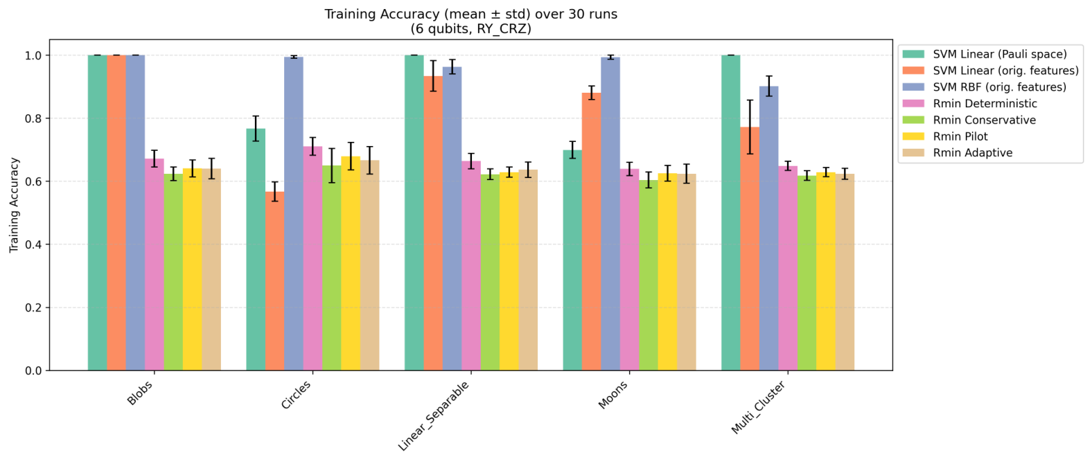
Figure 1 displays these accuracy results graphically. For reference, it also includes classical SVM baselines trained on the original input features. Across all datasets, the deterministic $R_{min}$ remains below the accuracy of the linear SVM trained on the full Pauli feature space. This observation is consistent with Theorem 1.

The computational savings are substantial. Evaluating all 4096 axes deterministically took on average 1098 s per dataset. The Conservative method, using only 60 axes, required about 16 s, corresponding to a speedup factor of approximately $68\times$. The Pilot and Adaptive methods achieved speedups of approximately $27\times$ and $36\times$, respectively, while generally producing estimates closer to the deterministic $R_{min}$ than the Conservative method. These results illustrate the practical advantage of Monte Carlo axis selection in simulated quantum-kernel workflows.

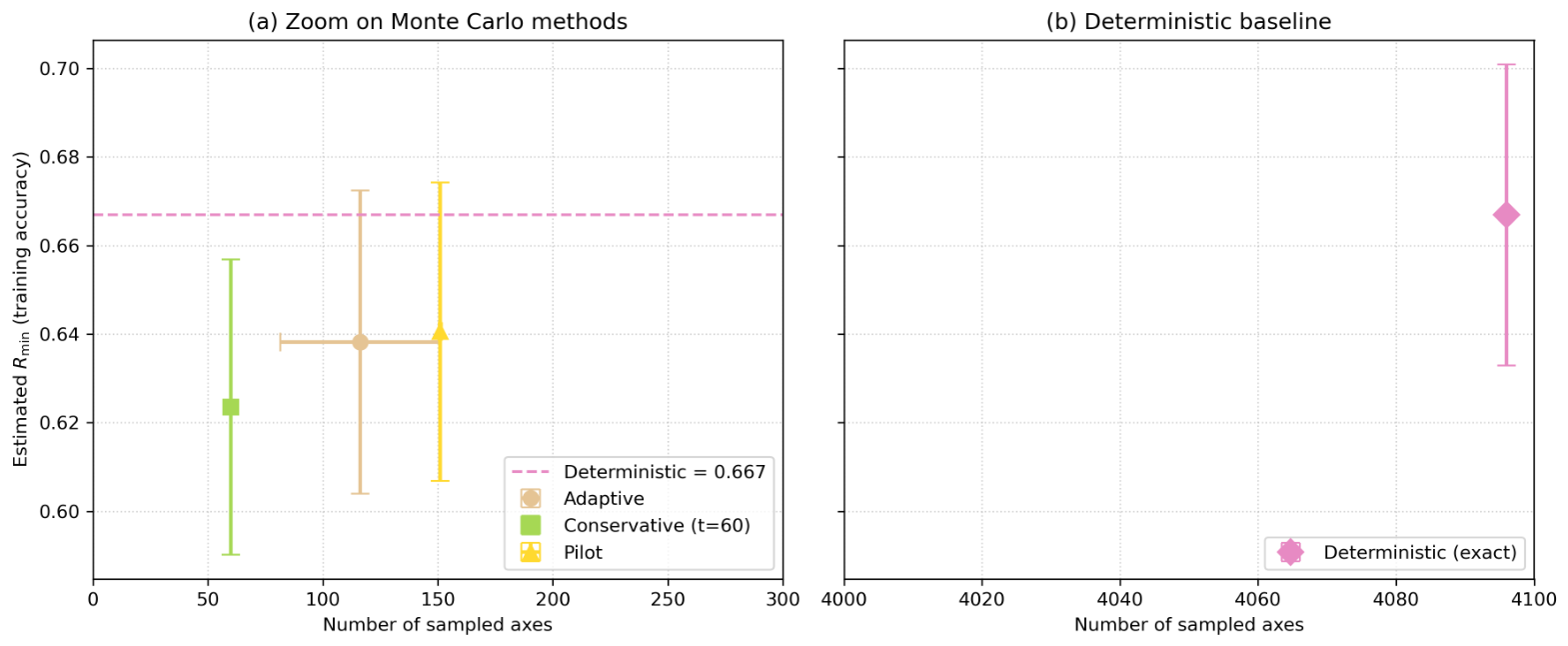
Figure 2 illustrates the trade-off between the number of sampled axes and the estimated value of $R_{min}$. The Monte Carlo methods concentrate near the low-cost region of the plot, while the deterministic scan evaluates all 4096 axes. The Pilot and Adaptive methods provide a favorable compromise between computational cost and proximity to the deterministic value, whereas the Conservative method gives a low-cost lower-bound estimate with the conditional coverage guarantee described in Corollary 1.

6.3. Discussion

The empirical results indicate that $R_{min}$ can serve as a useful training-free indicator of axis-aligned separability in the Pauli feature space for the settings considered in this study. The deterministic value of $R_{min}$ provides the exact optimum over Pauli-feature axes, while the Monte Carlo estimates remain lower bounds by construction and approach the deterministic value in the tested datasets.

The Conservative method offers a low-cost estimate by sampling only 60 axes. The Pilot and Adaptive methods typically yield estimates closer to the deterministic $R_{min}$ at a moderately higher computational cost, making them useful when a tighter lower-bound estimate is desired. The observed speedups highlight the practical value of Monte Carlo axis selection for simulated quantum-kernel workflows.

The comparison with the linear SVM trained on the full Pauli feature space is consistent with the theoretical inequality $R_{min}\le R^{*}$ proved in Theorem 1. This comparison should nevertheless be read in light of the distinction between the ideal optimum $R^{*}$ and the regularized objective optimized by a soft-margin SVM. Finally, the present experiments are limited to synthetic binary datasets, one family of quantum feature maps, and exact statevector simulations. Therefore, the results should be interpreted as evidence of the usefulness of the proposed framework in controlled settings, rather than as a general performance guarantee for arbitrary datasets, noisy devices, or all quantum feature maps.

To test the robustness of the proposed framework to hardware noise, we repeated the experiments under a depolarization noise model with error rate $p_{\mathrm{noise}}=0.02$, corresponding to a typical gate error for NISQ devices. The results, based on 30 complete repetitions, are reported in Appendix B.

Table A1. Mean training accuracy (±std) under a $2\%$ depolarization noise model for $n=6$ qubits ($d=4096$). Results based on 30 complete repetitions.

Dataset	Det. ${\mathit{R}}_{min}$	Cons. (60)	Pilot	Adaptive	SVM Pauli
Blobs	$0.670\pm 0.028$	$0.625\pm 0.023$	$0.631\pm 0.022$	$0.635\pm 0.026$	$1.000\pm 0.000$
Circles	$0.710\pm 0.027$	$0.635\pm 0.043$	$0.681\pm 0.044$	$0.667\pm 0.053$	$0.767\pm 0.040$
Linear_Sep	$0.668\pm 0.026$	$0.620\pm 0.016$	$0.629\pm 0.023$	$0.625\pm 0.016$	$1.000\pm 0.000$
Moons	$0.638\pm 0.020$	$0.607\pm 0.022$	$0.625\pm 0.021$	$0.627\pm 0.024$	$0.700\pm 0.029$
Multi_Cluster	$0.648\pm 0.016$	$0.621\pm 0.017$	$0.630\pm 0.017$	$0.623\pm 0.016$	$1.000\pm 0.000$

shows that the deterministic $R_{min}$ remains a valid lower bound on the linear SVM accuracy under noise, with degradation of less than $1\%$ compared to the noiseless case (

Table A2. Comparison of deterministic $R_{min}$: noiseless (30 runs) vs. $2\%$ depolarization noise (30 runs).

Dataset	Noiseless Det. ${\mathit{R}}_{min}$	Noisy Det. ${\mathit{R}}_{min}$	Degradation
Blobs	$0.672\pm 0.027$	$0.670\pm 0.028$	$0.3\%$
Circles	$0.711\pm 0.028$	$0.710\pm 0.027$	$0.1\%$
Linear_Separable	$0.664\pm 0.024$	$0.668\pm 0.026$	$-0.6\%$
Moons	$0.639\pm 0.021$	$0.638\pm 0.020$	$0.2\%$
Multi_Cluster	$0.649\pm 0.015$	$0.648\pm 0.016$	$0.2\%$

). For instance, on the Blobs dataset, the deterministic $R_{min}$ is $0.670\pm 0.028$ under noise, compared to $0.672\pm 0.027$ in the noiseless case—a difference well within the statistical variability. On the Circles dataset, the noisy value is $0.710\pm 0.027$, nearly identical to the noiseless $0.711\pm 0.028$. The Monte Carlo estimators continue to produce lower-bound estimates, with the Pilot method achieving estimates particularly close to the deterministic value (e.g., $0.681\pm 0.044$ vs. $0.710\pm 0.027$ for Circles, and $0.631\pm 0.022$ vs. $0.670\pm 0.028$ for Blobs).

These results demonstrate that the proposed framework is resilient to moderate levels of depolarizing noise. The accuracy degradation is negligible, and the lower-bound property—the central theoretical contribution of this work—remains intact under noise. This resilience reinforces the practical relevance of the proposed metric for near-term quantum devices.

7. Conclusions

This work establishes a rigorous theoretical and practical foundation for the minimum accuracy metric in quantum kernel methods. We generalized the original heuristic to arbitrary binary datasets and formally proved that $R_{min}$ is a certified lower bound on the optimal empirical accuracy achievable by any linear classifier in the same feature space (Theorem 1). Moreover, we introduced Monte Carlo axis-selection strategies, namely Conservative, Pilot, and Adaptive, that produce efficient lower-bound estimates of $R_{min}$. The Conservative strategy is supported by the quantile-coverage guarantee in Theorem 3 and Corollary 1, while the Pilot and Adaptive strategies provide practical heuristic variants.

Our experiments with $n=6$ qubits ($d=4096$) and 30 independent runs on five synthetic datasets show that:

• The Monte Carlo estimators sample as few as 60 axes while producing lower bounds by construction that, in the tested datasets, remain close to the exact $R_{min}$.
• The computational speedups range from approximately $27\times$ to $68\times$ compared to an exhaustive deterministic scan.
• The comparison with the linear SVM trained on the full Pauli feature space is consistent with the theoretical inequality $R_{min}\le R^{*}$.

These contributions transform the minimum accuracy from a heuristic into a scalable, theoretically sound tool for pre-screening quantum feature maps in simulated quantum-kernel pipelines.

Looking ahead, several directions are worth pursuing. We plan to extend the framework to multiclass problems, explore hybrid strategies that favor low-weight Pauli observables, and test $R_{min}$ as a practical screening tool for QAS [22,23,24]. We also aim to derive generalization bounds connecting the empirical $R_{min}$ to test performance. A crucial next step is validation on real quantum hardware and noisy simulators, where we can assess the impact of finite-shot statistics, decoherence, and readout errors. Finally, we intend to systematically evaluate $R_{min}$ across a wider range of feature-map architectures and real-world benchmark datasets.

References

1. Russell, S.; Norvig, P. Artificial Intelligence: A Modern Approach, 3rd ed.; Prentice Hall: New York, NY, USA, 2010. [Google Scholar]
2. Ciliberto, C.; Herbster, M.; Ialongo, A.D.; Pontil, M.; Rocchetto, A.; Severini, S.; Wossnig, L. Quantum machine learning: A classical perspective. Proc. R. Soc. A Math. Phys. Eng. Sci. 2018, 474, 20170551. [Google Scholar] [CrossRef] [Scilit]
3. El Ayachi, F.; El Baz, M. Enhancing quantum support vector machines using multipartite entanglement. Phys. Lett. A 2025, 551, 130666. [Google Scholar] [CrossRef] [Scilit]
4. Schuld, M.; Petruccione, F. Supervised Learning with Quantum Computers; Springer: Berlin/Heidelberg, Germany, 2018. [Google Scholar]
5. Wang, Y.; Qi, B.; Wang, X.; Liu, T.; Dong, D. Power characterization of noisy quantum kernels. IEEE Trans. Neural Netw. Learn. Syst. 2025, 36, 13939–13952. [Google Scholar] [CrossRef] [Scilit] [PubMed]
6. Havlíček, V.; Córcoles, A.D.; Temme, K.; Harrow, A.W.; Kandala, A.; Chow, J.M.; Gambetta, J.M. Supervised learning with quantum-enhanced feature spaces. Nature 2019, 567, 209–212. [Google Scholar] [CrossRef] [Scilit] [PubMed]
7. Schuld, M.; Killoran, N. Quantum machine learning in feature Hilbert spaces. Phys. Rev. Lett. 2019, 122, 040504. [Google Scholar] [CrossRef] [Scilit] [PubMed]
8. Liu, Y.; Arunachalam, S.; Temme, K. A rigorous and robust quantum speed-up in supervised machine learning. Nat. Phys. 2021, 17, 1013–1017. [Google Scholar] [CrossRef] [Scilit]
9. Miroszewski, A.; Asiani, M.F.; Mielczarek, J.; Le Saux, B.; Nalepa, J. In search of quantum advantage: Estimating the number of shots in quantum kernel methods. arXiv 2024, arXiv:2407.15776. [Google Scholar]
10. Kübler, J.M.; Buchholz, S.; Schölkopf, B. The Inductive Bias of Quantum Kernels. Adv. Neural Inf. Process. Syst. 2021, 34, 12661–12673. [Google Scholar]
11. Shaydulin, R.; Wild, S.M. Importance of kernel bandwidth in quantum machine learning. Phys. Rev. A 2022, 106, 042407. [Google Scholar] [CrossRef] [Scilit]
12. Canatar, A.; Peters, E.; Pehlevan, C.; Wild, S.M.; Shaydulin, R. Bandwidth Enables Generalization in Quantum Kernel Models. Trans. Mach. Learn. Res. 2023. Available online: https://openreview.net/forum?id=A1N2qp4yAq (accessed on 19 July 2026).
13. Thanasilp, S.; Wang, S.; Cerezo, M.; Holmes, Z. Exponential concentration in quantum kernel methods. Nat. Commun. 2024, 15, 5200. [Google Scholar] [CrossRef] [Scilit] [PubMed]
14. Schnabel, J.; Roth, M. Quantum kernel methods under scrutiny: A benchmarking study. Quantum Mach. Intell. 2024, 7, 58. [Google Scholar]
15. Álvarez-Estévez, D. Benchmarking Quantum Machine Learning Kernel Training for Classification Tasks. IEEE Trans. Quantum Eng. 2025, 6, 2500215. [Google Scholar] [CrossRef] [Scilit]
16. Cristianini, N.; Shawe-Taylor, J.; Elisseeff, A.; Kandola, J. On Kernel-Target Alignment. Adv. Neural Inf. Process. Syst. 2002, 14, 367–373. [Google Scholar] [CrossRef] [Scilit]
17. Hubregtsen, T.; Wierichs, D.; Gil-Fuster, E.; Derks, P.-J.H.S.; Faehrmann, P.K.; Meyer, J.J. Training quantum embedding kernels on near-term quantum computers. Phys. Rev. A 2022, 106, 042431. [Google Scholar] [CrossRef] [Scilit]
18. Pellow-Jarman, R.; Pillay, A.; Sinayskiy, I.; Petruccione, F. Hybrid genetic optimization for quantum feature map design. Quantum Mach. Intell. 2024, 6, 45. [Google Scholar] [CrossRef] [Scilit]
19. Salmenperä, I.; Kuhtarskis, I.; Meijer-van de Griend, A.; Nurminen, J.K. The impact of feature embedding placement in the ansatz of a quantum kernel in QSVMs. arXiv 2024, arXiv:2409.13147. [Google Scholar]
20. Gentinetta, G.; Sutter, D.; Zoufal, C.; Fuller, B.; Woerner, S. Quantum Kernel Alignment with Stochastic Gradient Descent. In Proceedings of the 2023 IEEE International Conference on Quantum Computing and Engineering (QCE); IEEE: New York, NY, USA, 2023; pp. 256–262. [Google Scholar]
21. Hur, T.; Araujo, I.F.; Park, D.K. Neural quantum embedding: Pushing the limits of quantum supervised learning. Phys. Rev. A 2024, 110, 022411. [Google Scholar] [CrossRef] [Scilit]
22. Sun, Y.; Wu, Z.; Tresp, V.; Ma, Y. Quantum Architecture Search with Unsupervised Representation Learning. Quantum 2026, 10, 1994. [Google Scholar]
23. Situ, H.; Li, G.; Li, Z.; He, Z.; Li, Y.; Li, L. Data-efficient predictor-based quantum architecture search with semi-supervised learning. Phys. Rev. A 2026, 113, 012402. [Google Scholar] [CrossRef] [Scilit]
24. Kundu, A.; Sarra, L. Reinforcement learning with learned gadgets to tackle hard quantum problems on real hardware. Commun. Phys. 2026, 9, 44. [Google Scholar] [CrossRef] [Scilit]
25. Cerezo, M.; Verdon, G.; Huang, H.-Y.; Cincio, L.; Coles, P.J. Challenges and opportunities in quantum machine learning. Nat. Comput. Sci. 2022, 2, 567–576. [Google Scholar] [CrossRef] [Scilit] [PubMed]
26. Schuld, M. Supervised quantum machine learning models are kernel methods. arXiv 2021, arXiv:2101.11020. [Google Scholar]
27. Jerbi, S.; Fiderer, L.J.; Nautrup, H.P.; Kübler, J.M.; Briegel, H.J.; Dunjko, V. Quantum machine learning beyond kernel methods. Nat. Commun. 2023, 14, 517. [Google Scholar] [CrossRef] [Scilit] [PubMed]
28. Suzuki, Y.; Yano, H.; Gao, Q.; Uno, S.; Tanaka, T.; Akiyama, M.; Yamamoto, N. Analysis and synthesis of feature map for kernel-based quantum classifier. Quantum Mach. Intell. 2020, 2, 9. [Google Scholar] [CrossRef] [Scilit]
29. Rubinstein, R.Y.; Kroese, D.P. Simulation and the Monte Carlo Method; John Wiley & Sons: Hoboken, NJ, USA, 2016. [Google Scholar]
30. Gentinetta, G.; Thomsen, A.; Sutter, D.; Woerner, S. The complexity of quantum support vector machines. Quantum 2024, 8, 1225. [Google Scholar] [CrossRef] [Scilit]
31. Huang, H.-Y.; Broughton, M.; Mohseni, M.; Babbush, R.; Boixo, S.; Neven, H.; McClean, J.R. Power of data in quantum machine learning. Nat. Commun. 2021, 12, 2631. [Google Scholar] [CrossRef] [Scilit] [PubMed]
32. Pedregosa, F.; Varoquaux, G.; Gramfort, A.; Michel, V.; Thirion, B.; Grisel, O.; Blondel, M.; Prettenhofer, P.; Weiss, R.; Dubourg, V.; et al. Scikit-learn: Machine learning in Python. J. Mach. Learn. Res. 2011, 12, 2825–2830. [Google Scholar]
Figure 1. Training accuracy (mean ± std) for each dataset and method. The deterministic R min is the exact axis-aligned value; Monte Carlo methods produce lower-bound estimates by construction. Classical SVM baselines on the original input features are included only for reference.
Quantumrep 08 00073 g001
Figure 2. Trade-off between the number of axes sampled and the resulting estimate of R min (mean ± std) over 30 runs. (a) Zoom on the low-cost region (0–300 axes) to clearly distinguish the Monte Carlo variants: Conservative ( t = 60 ), Pilot, and Adaptive. The dashed horizontal line indicates the exact deterministic value R min for reference. (b) Deterministic baseline evaluated on all 4096 Pauli-feature axes, giving the exact R min .
Quantumrep 08 00073 g002