Spin–Position Entanglement Entropy in Stern–Gerlach Dynamics: Exact Overlap Law and Gaussian Phase–Space Reductions

Abstract

We derive the reduced-spin von Neumann entropy generated by unitary Stern–Gerlach spin–position entanglement in a closed system. For any pure two-branch state with normalized spatial branches, the reduced-spin spectrum and entropy are determined entirely by the initial spin population p and the magnitude |γ| of the spatial branch overlap. This constitutes an exact, model-independent two-branch overlap law. For equal-width, unchirped Gaussian branches, |γ| = exp(−κ), where κ = Δx²/(8σ_x²) + σ_x²Δp²/(2ℏ²) is a quadratic phase-space distinguishability parameter that combines relative position and momentum displacements. The Gaussian entropy can therefore be written as S_s(κ,p), although this particular phase-space expression for κ does not generally apply to arbitrary wave-packet shapes. We derive the reduced density matrix and its spectrum, the equal-width Gaussian reduction, the constant-gradient form of κ(t), the weak-distinguishability onset and saturation limits, and an entropy response function. We also derive the overlap for freely spreading, chirped equal-width Gaussians and for unequal-width unchirped Gaussians, for which the fixed-width parameter κ is replaced by the corresponding Gaussian overlap coordinate. Different apparatus settings generally produce different entropy trajectories in time; at a fixed input population, these trajectories collapse only after reparametrization in terms of the appropriate overlap coordinate.

1. Introduction and Contribution

The present analysis uses standard concepts from quantum mechanics, quantum measurement, decoherence theory, and quantum information [1,2,3,4,5,6,7]. A Stern–Gerlach apparatus is commonly introduced as a device that spatially separates spin components, following the original observation of spatial quantization in an inhomogeneous magnetic field [8]. From a quantum–mechanical perspective, the essential process is unitary spin–position entanglement. An initially coherent spin superposition becomes correlated with two spatial wave packets. When the packets overlap strongly, the reduced spin state remains nearly pure; as they become distinguishable, tracing over position renders the reduced spin state mixed. The corresponding von Neumann entropy therefore quantifies the spin coherence transferred into spin–position correlations.

The connection among Stern–Gerlach separation, wave-packet overlap, and spin coherence is well established. Previous studies have examined coherence recovery, environmental and dissipative Stern–Gerlach dynamics, Wigner matrix descriptions, and finite-resolution measurements [9,10,11,12,13,14,15]. Coherent Stern–Gerlach momentum splitting and complete Stern–Gerlach interferometry have also been realized experimentally [16,17], underscoring the relevance of both position and momentum separation. The contribution of the present work is therefore not the general observation that overlap matters, but an explicit entropy parametrization with a clearly defined domain of validity. First, the reduced-spin spectrum is written directly as an exact two-branch function of the initial population p and the overlap magnitude |γ|. Second, for a specified family of equal-width Gaussian packets, |γ| is reduced to a single quadratic phase-space coordinate κ. Third, the same overlap-based framework is extended to freely spreading chirped Gaussians and to unequal-width Gaussians, for which the appropriate Gaussian coordinate is modified. The result is thus a precise entropy parametrization with an explicit domain of validity, rather than a new mechanism of Stern–Gerlach decoherence.

Throughout this work, the term universal is used only in the following restricted sense. The exact entropy law S_s = S_s(|γ|,p) holds for any normalized pair of pure spatial branches in a closed, two-branch system. By contrast, the representation |γ| = exp(−κ), with κ expressed as a quadratic function of relative position and momentum, is specific to the Gaussian packet families considered here. Although one may formally define κ = −ln|γ| whenever |γ| > 0, this definition is not, in general, a shape-independent phase-space distance.

The von Neumann entropy is used here because, for the globally pure spin–position states considered in this work, the entropy of the reduced spin state is exactly the bipartite entanglement entropy. It is basis-independent, vanishes if and only if the spin and spatial degrees of freedom are unentangled, and is bounded by ln 2 for the spin-1/2 subsystem. Unlike a single coherence component, it combines the effects of population imbalance and coherence into the spectrum of the reduced state. For fixed p, it is a monotonic function of |γ|, so it does not replace the overlap as microscopic information; rather, it provides a common scalar scale on which different Stern–Gerlach regimes can be compared in terms of spin–position entanglement.

Scope and Assumptions

The assumptions underlying the various formulas are summarized here to make the domain of each result explicit.

• The model retains one spatial coordinate x along the magnetic field gradient; transverse motion is factored out. The linear field used below should be understood as a local effective description of the relevant field component over the spatial support of the packet, not as a globally one-dimensional magnetic field.
• The total spin–position system is closed and evolves unitarily. Detector coarse-graining, environmental decoherence, and mixed initial spatial states lie outside the scope of the present model.
• The spin degree of freedom is a two-level system initially prepared in a pure superposition with population p = |c↑|². The spatial branch states are normalized.
• The constant-gradient example assumes a linearized magnetic field, equal initial branch centers, and equal initial mean momenta.
• Section 5, Section 6 and Section 9 use equal-width, unchirped Gaussian branches. Section 7 allows for a common time-dependent width and a common chirp, whereas Section 8 allows for unequal widths but assumes zero chirp.

2. Stern–Gerlach Hamiltonian and Spin-Conditioned Motion

Consider the standard one-dimensional Stern–Gerlach Hamiltonian

$$H={\displaystyle \frac{{\widehat{p}}^2}{2m}}-{\mu }_m{\widehat{\sigma }}_{z}B\left(x\right),$$

(1)

where μ_m is the relevant magnetic moment scale and B(x) is the magnetic field component along the spin-quantization axis. Linearizing the field within the interaction region,

$$B\left(x\right)=B_0+B^{\prime }x$$

(2)

and, apart from a spin-dependent but entropy-irrelevant phase generated by B₀, the interaction reduces to the force Hamiltonian

$$H_{\mathrm{i}\mathrm{n}\mathrm{t}}=-{\mu }_m{B}^{\prime }x{\widehat{\sigma }}_z.$$

(3)

The two spin components experience equal and opposite forces:

$$F_{\uparrow }=+F, F_{\downarrow }=-F, F={\mu }_m{B}^{\prime }$$

(4)

Choosing the common initial center and mean momentum as zero (equivalently, working in the comoving frame), the branch centers obey

$$x_{\uparrow }\left(t\right)={\displaystyle \frac{F}{2m}}{t}^2, x_{\downarrow }\left(t\right)=-{\displaystyle \frac{F}{2m}}{t}^2$$

(5)

$$p_{\uparrow }\left(t\right)=Ft, p_{\downarrow }\left(t\right)=-Ft,$$

(6)

The corresponding relative displacements are therefore

$$\Delta x\left(t\right)={\displaystyle \frac{F}{m}}{t}^2, \Delta p\left(t\right)=2Ft.$$

(7)

Although Equations (5)–(7) have the form of classical constant-force trajectories, no semiclassical substitution is involved. For the exact branch Hamiltonians H± = $\widehat{p}$²/(2m) ∓ Fx, the Heisenberg equations are operator identities: d $\widehat{p}$±/dt = ±F and d $\widehat{x}$±/dt = $\widehat{p}$±/m. Their integration gives $\widehat{p}$±(t) = $\widehat{p}$(0) ± Ft and $\widehat{x}$±(t) = $\widehat{x}$(0) + $\widehat{p}$(0)t/m ± Ft²/(2m). Thus, Δp(t) = 2 Ft and Δx(t) = Ft²/m are exact quantum displacement parameters. The linear force shifts only the first moments, while both branches undergo the same covariance evolution under the kinetic term. Consequently, using Δx(t) and Δp(t) in the Gaussian overlap introduces no classical approximation into the quantum calculation [2].

The exact constant-force propagator also contains a dynamical phase that is cubic in time. In the symmetric ±F model considered here, the cubic contribution is proportional to F² and is therefore the same for the two branches; as a common global phase, it cancels from the branch overlap γ. The force-odd part of the evolution instead appears through the relative displacement and relative phase, including the momentum separation Δp. If the two branches experience unequal force magnitudes, unequal interaction times, or additional spin-dependent potentials, a residual relative dynamical phase can survive in arg γ. The entropy studied here is insensitive to that phase because it depends only on |γ|, but the phase remains present in the off-diagonal coherence ρ↑↓ = c↑c↓*γ and can therefore be accessed through complete spin-state tomography or an interferometric recombination measurement.

3. General Spin–Position State

After the Stern–Gerlach evolution, write the joint pure state as

$$\left|\Psi \left(t\right)⟩=c_{\uparrow }\right|\uparrow ⟩\left|{\varphi }_{\uparrow }\left(t\right)⟩+c_{\downarrow }\right|\downarrow ⟩|{\varphi }_{\downarrow }\left(t\right)⟩,$$

(8)

with

$${\left|c_{\uparrow }\right|}^2+{\left|c_{\downarrow }\right|}^2=1, ⟨{\varphi }_j\left(t\right)|{\varphi }_j\left(t\right)⟩=1 \left(j=\uparrow ,\downarrow \right).$$

(9)

Define the branch overlap as

$$\gamma \left(t\right)=⟨{\varphi }_{\downarrow }\left(t\right)|{\varphi }_{\uparrow }\left(t\right)⟩.$$

(10)

Define the full density operator ρ(t) = |Ψ(t)⟩⟨Ψ(t)|. The reduced spin state is obtained by tracing over the spatial Hilbert space:

$${\rho }_s\left(t\right)={\mathrm{T}\mathrm{r}}_x\rho \left(t\right)=\left(\begin{array}{cc}{\left|c_{\uparrow }\right|}^2& c_{\uparrow }{c}_{\downarrow }^{*}\gamma \left(t\right)\\ c_{\downarrow }{c}_{\uparrow }^{*}{\gamma }^{*}\left(t\right)& {\left|c_{\downarrow }\right|}^2\end{array}\right)$$

(11)

Here, Tr_x denotes the partial trace over the spatial Hilbert space. This operation removes the spatial degrees of freedom while leaving an operator on the remaining two-dimensional spin Hilbert space; therefore, Tr_xρ is a 2 × 2 matrix. This should be distinguished from the ordinary trace of the reduced matrix, which is the scalar Tr_sρ_s = |c↑|² + |c↓|² = 1. Equation (11) is therefore a reduced-density-matrix identity, not an identification of a scalar trace with a matrix.

The diagonal populations remain unchanged, whereas the off-diagonal spin coherence is multiplied by the spatial overlap. This result follows solely from the two-branch pure-state structure in Equation (8) and does not require Gaussian wave packets.

4. Exact Two-Branch Overlap Law

Let

$$p={\left|c_{\uparrow }\right|}^2, 1-p={\left|c_{\downarrow }\right|}^2.$$

(12)

For later use, the determinant of the reduced spin matrix is

$$\mathrm{d}\mathrm{e}\mathrm{t}{\rho }_s=p\left(1-p\right)\left(1-{\left|\gamma \right|}^2\right).$$

(13)

The determinant det ρ_s in Equation (13) is not itself set equal to zero; rather, it appears as the constant term in the characteristic polynomial. The eigenvalues are obtained from det(ρ_s − λI) = 0. Because Tr_sρ_s = 1, the characteristic equation becomes λ² − λ + detρ_s = 0, or equivalently λ² − λ + p(1 − p)(1 − |γ|²) = 0.

The two reduced-spin eigenvalues are therefore

$${\lambda }_{\pm }\left(\left|\gamma \right|,p\right)={\displaystyle \frac{1}{2}}\left[1\pm \sqrt{1-4p\left(1-p\right)\left(1-{\left|\gamma \right|}^2\right)}\right].$$

(14)

The reduced-spin von Neumann entropy is

S_s(|γ|, p) = −λ₊ ln λ₊ − λ₋ ln λ_−.

(15)

Proposition 1 

(exact two-branch overlap law). For any normalized pure state of the form in Equation (8), the reduced-spin spectrum and entropy are fixed by the pair (p, |γ|) through Equations (14) and (15). This is the exact sense in which the entropy law is universal: it is independent of the detailed spatial shape once the branch-overlap magnitude is specified. No Gaussian assumption has entered this result.

5. Equal-Width Gaussian Overlap and Phase-Space Reduction

We now specialize to two equal-width, unchirped Gaussian packets:

$${\varphi }_{\uparrow }\left(x,t\right)={\displaystyle \frac{1}{{\left(2\pi {\sigma }_x^2\right)}^{1/4}}}\mathrm{e}\mathrm{x}\mathrm{p}\left[-{\displaystyle \frac{{\left(x-x_{\uparrow }\right)}^2}{4{\sigma }_x^2}}+{\displaystyle \frac{i}{\mathrm{\hslash }}}{p}_{\uparrow }x\right]$$

(16)

$${\varphi }_{\downarrow }\left(x,t\right)={\displaystyle \frac{1}{{\left(2\pi {\sigma }_x^2\right)}^{1/4}}}\mathrm{e}\mathrm{x}\mathrm{p}\left[-{\displaystyle \frac{{\left(x-x_{\downarrow }\right)}^2}{4{\sigma }_x^2}}+{\displaystyle \frac{i}{\mathrm{\hslash }}}{p}_{\downarrow }x\right]$$

(17)

Let Δx = x↑ − x↓, $\stackrel{\mathrm{‾}}{\mathrm{x}}$ = (x↑ + x↓)/2, and Δp = p↑ − p↓. The overlap integral can then be written as

$$\gamma ={\displaystyle \frac{1}{\sqrt{2\pi {\sigma }_x^2}}}{\int }_{-\mathrm{\infty }}^{\mathrm{\infty }}\mathrm{e}\mathrm{x}\mathrm{p}\left[-{\displaystyle \frac{{\left(x-x_{\uparrow }\right)}^2+{\left(x-x_{\downarrow }\right)}^2}{4{\sigma }_x^2}}+{\displaystyle \frac{i\Delta p}{\mathrm{\hslash }}}x\right]dx$$

(18)

$$\begin{array}{c}\gamma =\mathrm{e}\mathrm{x}\mathrm{p}\left[-{\displaystyle \frac{{\left(\Delta x\right)}^2}{8{\sigma }_x^2}}+{\displaystyle \frac{i\Delta p\hspace{0.17em}\bar{x}}{\mathrm{\hslash }}}\right]\\ \times {\displaystyle \frac{1}{\sqrt{2\pi {\sigma }_x^2}}}{\int }_{-\mathrm{\infty }}^{\mathrm{\infty }}\mathrm{e}\mathrm{x}\mathrm{p}\left[-{\displaystyle \frac{{\left(x-\bar{x}\right)}^2}{2{\sigma }_x^2}}+{\displaystyle \frac{i\Delta p}{\mathrm{\hslash }}}\left(x-\bar{x}\right)\right]dx\end{array}.$$

(19)

Evaluating the integral with the Gaussian Fourier transform gives

$$\gamma =\mathrm{e}\mathrm{x}\mathrm{p}\left[-{\displaystyle \frac{\Delta x^2}{8{\sigma }_x^2}}-{\displaystyle \frac{{\sigma }_x^2\Delta p^2}{2{\mathrm{\hslash }}^2}}+{\displaystyle \frac{i\Delta p\hspace{0.17em}\bar{x}}{\mathrm{\hslash }}}\right].$$

(20)

Hence

$$\left|\gamma \right|=e^{-\kappa }, \kappa ={\displaystyle \frac{\Delta x^2}{8{\sigma }_x^2}}+{\displaystyle \frac{{\sigma }_x^2\Delta p^2}{2{\mathrm{\hslash }}^2}}.$$

(21)

The entropy depends only on the magnitude of γ and is therefore insensitive to its phase. Equation (21) is a phase-space reduction specific to this equal-width Gaussian family and should not be interpreted as an identity for arbitrary wave packets.

To make the terminology precise, distinguishability refers here specifically to the two normalized spatial branch states |φ↑⟩ and |φ↓⟩, rather than to the spin populations or to an externally imposed measurement strength. Three equivalent quantities are useful: the overlap magnitude |γ| = |⟨φ↓|φ↑⟩|, the branch fidelity F_br = |γ|², and the pure-state trace distance D = √(1 − F_br) = √(1 − |γ|²). Thus, D = 0 for identical normalized branches (|γ| = 1) and D → 1 as the branches become orthogonal (|γ| → 0). In this work, weak distinguishability denotes D ≪ 1, equivalently |γ| ≈ 1; for the equal-width Gaussian family, this corresponds to κ ≪ 1 because |γ| = exp(−κ). Strong distinguishability denotes D → 1, equivalently |γ| → 0 and, within that Gaussian family, κ → ∞.

6. Gaussian Entropy Parametrization

Substituting |γ| = exp(−κ) into Equation (14) gives

$${\lambda }_{\pm }\left(\kappa ,p\right)={\displaystyle \frac{1}{2}}\left[1\pm \sqrt{1-4p\left(1-p\right)\left(1-e^{-2\kappa }\right)}\right]$$

(22)

and

S_s(κ, p) = −λ₊(κ, p) ln λ₊(κ, p) − λ₋(κ, p) ln λ₋(κ, p).

(23)

Proposition 2 

(equal-width Gaussian reduction). For the packet family in Section 5, the exact two-branch overlap law can be parametrized by the single Gaussian phase-space coordinate κ in Equation (21). The separate quantities Δx, Δp, and σ_x enter the reduced-spin entropy only through κ.

For a balanced spin superposition, p = 1/2, Equation (22) simplifies exactly rather than asymptotically. Because 4p(1 − p) = 1, the square root in Equation (22) becomes √{1 − [1 − exp(−2κ)]} = √{exp(−2κ)} = exp(−κ), since κ ≥ 0. Therefore, λ± = [1 ± exp(−κ)]/2 exactly. Equation (24) is thus a direct algebraic specialization of Equation (22), and Equation (25) follows by substituting these exact eigenvalues into the von Neumann entropy. 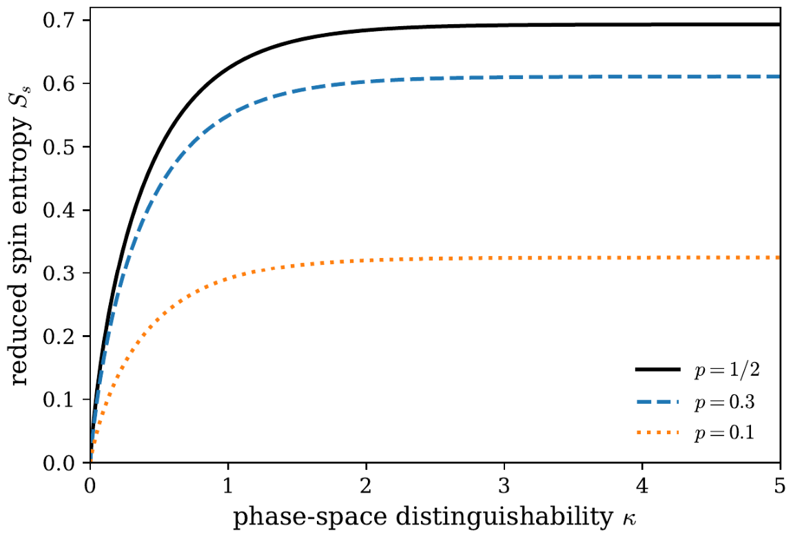Figure 1 displays the resulting entropy curves for representative values of p.

$${\lambda }_{\pm }\left(\kappa \right)={\displaystyle \frac{1}{2}}\left(1\pm e^{-\kappa }\right)$$

(24)

$$\begin{array}{c}{S}_s\left(\kappa \right)=-{\displaystyle \frac{1+e^{-\kappa }}{2}}\mathrm{l}\mathrm{n}\left({\displaystyle \frac{1+e^{-\kappa }}{2}}\right)\\ -{\displaystyle \frac{1-e^{-\kappa }}{2}}\mathrm{l}\mathrm{n}\left({\displaystyle \frac{1-e^{-\kappa }}{2}}\right)\end{array}$$

(25)

7. Time-Dependent Spreading and Chirped Gaussian Packets

The fixed-width expression in Equation (21) assumes a constant packet width σ_x and no quadratic phase chirp. It therefore describes the equal-time overlap of unchirped Gaussian packets rather than the dynamical propagation of freely evolving packets. Here, free spreading refers to the unitary broadening generated by the kinetic term $\widehat{p}$²/(2m). A Gaussian packet with initial width σ₀ develops both a time-dependent width σ_t and a correlated quadratic phase, or chirp. Both effects must be retained when evaluating the dynamical overlap. Define

$$\vartheta \left(t\right)={\displaystyle \frac{\mathrm{\hslash }t}{2m{\sigma }_0^2}}, {\sigma }_t={\sigma }_0\sqrt{1+\vartheta {\left(t\right)}^2}.$$

(26)

Consider two branches with the same instantaneous width σ_t and the same chirp θ(t),

$${\varphi }_j\left(x,t\right)={\displaystyle \frac{1}{{\left(2\pi {\sigma }_t^2\right)}^{1/4}}}\mathrm{e}\mathrm{x}\mathrm{p}\left[-{\displaystyle \frac{\left(1-i\vartheta \right){\left(x-x_j\right)}^2}{4{\sigma }_t^2}}+{\displaystyle \frac{i}{\mathrm{\hslash }}}{p}_{j}x\right], j=\uparrow ,\downarrow .$$

(27)

Derivation for Chirped Equal-Width Gaussians

Let y = x − $\stackrel{\mathrm{‾}}{\mathrm{x}}$, where $\stackrel{\mathrm{‾}}{\mathrm{x}}$ = (x↑ + x↓)/2. In the product φ↓*(x,t)φ↑(x,t), the real Gaussian part contributes −y²/(2σ_t²) − Δx²/(8σ_t²), while the common chirp modifies the coefficient of the linear phase. Up to an overall phase Φ(t),

$${\varphi }_{\downarrow }^{*}\left(x,t\right){\varphi }_{\uparrow }\left(x,t\right)\propto \mathrm{e}\mathrm{x}\mathrm{p}\left[-{\displaystyle \frac{y^2}{2{\sigma }_t^2}}-{\displaystyle \frac{\Delta x^2}{8{\sigma }_t^2}}+i\left({\displaystyle \frac{\Delta p}{\mathrm{\hslash }}}-{\displaystyle \frac{\vartheta \Delta x}{2{\sigma }_t^2}}\right)y+i\Phi \left(t\right)\right].$$

(28)

Applying the same Gaussian Fourier integral as above gives

$${\gamma }_{\mathrm{s}\mathrm{p}}\left(t\right)=\mathrm{e}\mathrm{x}\mathrm{p}\left[-{\kappa }_{\mathrm{s}\mathrm{p}}\left(t\right)+i\Phi \left(t\right)\right],$$

(29)

where

$${\kappa }_{\mathrm{s}\mathrm{p}}\left(t\right)={\displaystyle \frac{\Delta x{\left(t\right)}^2}{8{\sigma }_t^2}}+{\displaystyle \frac{{\sigma }_t^2}{2{\mathrm{\hslash }}^2}}{\left[\Delta p\left(t\right)-{\displaystyle \frac{\mathrm{\hslash }\vartheta \left(t\right)}{2{\sigma }_t^2}}\Delta x\left(t\right)\right]}^2.$$

(30)

The second term measures the momentum displacement relative to the local phase-space tilt of the spreading packet. Physically, the chirp θ(t) is the position–momentum correlation generated by free propagation: phase-space ellipses that are initially untilted become sheared, so a given spatial displacement is correlated with a phase gradient. The same result can be verified directly from the Gaussian covariance matrix. Each branch has Var(x) = σ_t², Cov(x,p) = ℏθ(t)/2, and Var(p) = ℏ²/(4σ₀²). For two pure Gaussian states with the same covariance matrix V_t and displacement vector δ = (Δx, Δp)ᵀ, the overlap magnitude is |γ| = exp[−δᵀV_t⁻¹δ/8]. Completing the square in this expression reproduces Equation (30), including the phase-correlation term Δp − ℏθ(t)Δx/(2σ_t²). The phase factor is therefore not an ad hoc correction, but the covariance representation of the exact Gaussian overlap. Experimentally, the packet centers and widths can be obtained from spatial imaging, whereas the chirp requires phase-sensitive information, for example from time-of-flight covariance reconstruction or interferometric/tomographic measurements. In the no-spreading limit, θ(t) → 0 and σ_t → σ₀, and Equation (30) reduces to Equation (21).

For the constant-gradient trajectories of Equation (7),

$${\kappa }_{\mathrm{s}\mathrm{p}}\left(t\right)={\displaystyle \frac{F^2{t}^4}{8m^2{\sigma }_t^2}}+{\displaystyle \frac{{\sigma }_t^2}{2{\mathrm{\hslash }}^2}}{\left[2Ft-{\displaystyle \frac{\mathrm{\hslash }\vartheta \left(t\right)F{t}^2}{2m{\sigma }_t^2}}\right]}^2.$$

(31)

For the constant-gradient displacements Δx = Ft²/m and Δp = 2 Ft, substituting θ(t) = ℏt/(2mσ₀²) and σ_t² = σ₀²[1 + θ(t)²] into Equation (31) gives exactly κ_sp(t) = F²t⁴/(8 m²σ₀²) + 2σ₀²F²t²/ℏ², which is identical to Equation (37). This equality provides an independent consistency check on the phase factor: free spreading changes the packet width and introduces a chirp, but these effects combine so that the exact overlap exponent for the uniformly forced branches agrees with the result obtained from the equivalent phase-space displacement. Consequently, all subsequent entropy formulas remain functions of the same exact overlap magnitude |γ(t)|.

The entropy then follows from the exact two-branch law by setting |γ(t)| = exp[−κ_sp(t)]. The entropy law itself is unchanged; only the Gaussian representation of the overlap has been modified.

8. Unequal-Width Gaussian Overlap

We next consider unchirped Gaussian packets with unequal widths,

$${\varphi }_j\left(x\right)={\displaystyle \frac{1}{{\left(2\pi {\sigma }_j^2\right)}^{1/4}}}\mathrm{e}\mathrm{x}\mathrm{p}\left[-{\displaystyle \frac{{\left(x-x_j\right)}^2}{4{\sigma }_j^2}}+{\displaystyle \frac{i}{\mathrm{\hslash }}}{p}_{j}x\right], j=\uparrow ,\downarrow .$$

(32)

Derivation for Unequal-Width Gaussians

Let Dσ = σ↑² + σ↓². The overlap exponent is a quadratic form Ax² + Bx + C, with

$$\begin{array}{ll}{D}_{\sigma }={\sigma }_{\uparrow }^2+{\sigma }_{\downarrow }^2,& A=-{\displaystyle \frac{D_{\sigma }}{4{\sigma }_{\uparrow }^2{\sigma }_{\downarrow }^2}},\\ B={\displaystyle \frac{x_{\uparrow }}{2{\sigma }_{\uparrow }^2}}+{\displaystyle \frac{x_{\downarrow }}{2{\sigma }_{\downarrow }^2}}+{\displaystyle \frac{i\Delta p}{\mathrm{\hslash }}},& C=-{\displaystyle \frac{x_{\uparrow }^2}{4{\sigma }_{\uparrow }^2}}-{\displaystyle \frac{x_{\downarrow }^2}{4{\sigma }_{\downarrow }^2}}\end{array}.$$

(33)

Evaluating the Gaussian integral and retaining its magnitude gives

$$\left|{\gamma }_{\mathrm{u}\mathrm{n}\mathrm{e}\mathrm{q}}\right|={\left({\displaystyle \frac{2{\sigma }_{\uparrow }{\sigma }_{\downarrow }}{{\sigma }_{\uparrow }^2+{\sigma }_{\downarrow }^2}}\right)}^{1/2}\mathrm{e}\mathrm{x}\mathrm{p}\left[-{\displaystyle \frac{\Delta x^2}{4\left({\sigma }_{\uparrow }^2+{\sigma }_{\downarrow }^2\right)}}-{\displaystyle \frac{{\sigma }_{\uparrow }^2{\sigma }_{\downarrow }^2\Delta p^2}{{\mathrm{\hslash }}^2\left({\sigma }_{\uparrow }^2+{\sigma }_{\downarrow }^2\right)}}\right].$$

(34)

Equivalently, define the unequal-width overlap coordinate as

$${\kappa }_{\mathrm{u}\mathrm{n}\mathrm{e}\mathrm{q}}={\displaystyle \frac{1}{2}}\mathrm{l}\mathrm{n}\left({\displaystyle \frac{{\sigma }_{\uparrow }^2+{\sigma }_{\downarrow }^2}{2{\sigma }_{\uparrow }{\sigma }_{\downarrow }}}\right)+{\displaystyle \frac{\Delta x^2}{4\left({\sigma }_{\uparrow }^2+{\sigma }_{\downarrow }^2\right)}}+{\displaystyle \frac{{\sigma }_{\uparrow }^2{\sigma }_{\downarrow }^2\Delta p^2}{{\mathrm{\hslash }}^2\left({\sigma }_{\uparrow }^2+{\sigma }_{\downarrow }^2\right)}}.$$

(35)

The logarithmic term represents distinguishability caused by a mismatch of packet widths: two Gaussian packets with different widths are already nonidentical even when Δx = Δp = 0. In the ideal symmetric linear-gradient model with identical initial covariances, the two branches retain equal widths, so this case is an extension rather than a feature generated by the minimal model itself. Unequal widths can arise from unequal state preparation, different focusing or propagation histories, spin-dependent lensing, or nonlinear magnetic field curvature that distorts the two branches differently. The widths are directly accessible from spatial profiles, while the resulting loss of spin coherence can be inferred from reduced-spin tomography. When σ↑ = σ↓ = σ_x, Equation (35) reduces to Equation (21).

9. Constant-Gradient Entropy Dynamics

Substituting Equation (7) into Equation (21) gives Equations (36) and (37). Here, the fixed-width symbol σ_x in Equation (21) is identified with the initial packet width σ₀ used in Section 7.

$$\kappa \left(t\right)={\displaystyle \frac{1}{8{\sigma }_x^2}}{\left({\displaystyle \frac{F}{m}}{t}^2\right)}^2+{\displaystyle \frac{{\sigma }_x^2}{2{\mathrm{\hslash }}^2}}{\left(2Ft\right)}^2$$

(36)

$$\kappa \left(t\right)={\displaystyle \frac{F^2{t}^4}{8m^2{\sigma }_x^2}}+{\displaystyle \frac{2{\sigma }_x^2{F}^2{t}^2}{{\mathrm{\hslash }}^2}}.$$

(37)

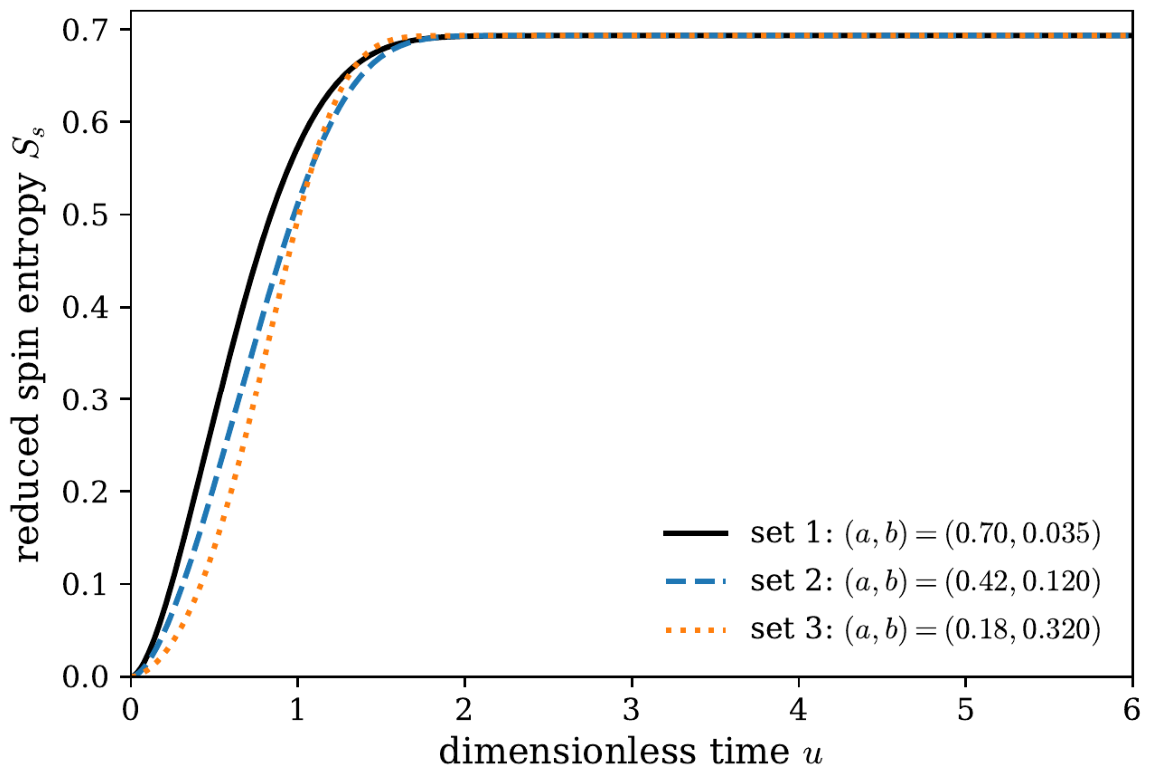
Thus κ(t) contains a t² contribution from momentum separation at early times and a t⁴ contribution from position separation. Figure 2 illustrates the corresponding time-domain behavior for three representative model parameter sets.

10. Weak-Distinguishability Onset and Nonanalyticity

For a balanced spin superposition (p = 1/2), Equation (24) is exact. The weak-distinguishability limit is obtained only afterward by expanding exp(−κ) for κ ≪ 1: exp(−κ) = 1 − κ + κ²/2 + O(κ³). Therefore, λ− = [1 − exp(−κ)]/2 = κ/2 − κ²/4 + O(κ³), whereas λ+ = [1 + exp(−κ)]/2 = 1 − κ/2 + κ²/4 + O(κ³). Equation (38) is therefore the leading term of a controlled expansion of the exact eigenvalues rather than an independent assumption.

λ₋(κ) = [1 − exp(−κ)]/2 ≈ κ/2, λ₊(κ) ≈ 1 − κ/2

(38)

Substituting these expansions into S_s = −λ+ ln λ+ − λ− ln λ− gives the leading weak-distinguishability asymptotics:

$$S_s\left(\kappa \right)\approx -{\displaystyle \frac{\kappa }{2}}\mathrm{l}\mathrm{n}\left({\displaystyle \frac{\kappa }{2}}\right)+{\displaystyle \frac{\kappa }{2}}, \kappa \ll 1, p={\displaystyle \frac{1}{2}}$$

(39)

More explicitly, the small eigenvalue contributes −λ− ln λ− = −(κ/2)ln(κ/2) + O(κ²|ln κ|), whereas the large eigenvalue contributes −λ+ ln λ+ = κ/2 + O(κ²). Hence S_s(κ) = −(κ/2)ln(κ/2) + κ/2 + O(κ²|ln κ|), which makes the remainder in Equation (39) explicit. For the constant-gradient model, κ(t) = At² + Bt⁴, with A = 2σ₀²F²/ℏ² and B = F²/(8 m²σ₀²). Therefore, S_s(t) = −(At²/2)ln(At²/2) + At²/2 + O(t⁴|ln t|). The logarithmic nonanalyticity is a generic property of the von Neumann entropy when an eigenvalue approaches zero, because of the function −x ln x at the boundary of state space; the specific t²|ln t| scaling is model-dependent and arises here because the small eigenvalue begins at order t². It is therefore not, by itself, a signature of weak measurement. In principle the behavior can be reconstructed from spin-state tomography, although resolving the very small eigenvalue close to a pure state is experimentally demanding.

11. Orthogonal-Branch (Strong-Distinguishability) Limit and Saturation

Because the present model describes closed, unitary spin–position entanglement and contains no projective detector operation, we use the term strong distinguishability rather than strong measurement. The limit considered below is therefore an orthogonal-branch limit defined solely by the overlap of the spatial states.

When |γ| → 0 (equivalently D → 1, or κ → ∞ within the relevant Gaussian family), the two normalized spatial branch states become orthogonal and the reduced spin state becomes diagonal,

$${\rho }_s\left(\mathrm{\infty }\right)=\left(\begin{array}{cc}p& 0\\ 0& 1-p\end{array}\right)$$

(40)

and

$$S_s\left(\mathrm{\infty }\right)=-p\mathrm{l}\mathrm{n}p-\left(1-p\right)\mathrm{l}\mathrm{n}\left(1-p\right).$$

(41)

For p = 1/2, the saturation value is ln 2, the maximum possible entropy of a two-level reduced state.

12. Entropy Response Function

Because S_s = S_s(κ,p) for the specified Gaussian parametrization,

$${\displaystyle \frac{d{S}_s}{dt}}={\displaystyle \frac{\mathsf{\partial }{S}_s}{\mathsf{\partial }\kappa }}{\displaystyle \frac{d\kappa }{dt}}.$$

(42)

Define

$$R_s\left(\kappa ,p\right)\equiv {\displaystyle \frac{\mathsf{\partial }{S}_s\left(\kappa ,p\right)}{\mathsf{\partial }\kappa }}.$$

(43)

For p = 1/2,

$$R_s\left(\kappa ,1/2\right)={\displaystyle \frac{e^{-\kappa }}{2}}\mathrm{l}\mathrm{n}\left({\displaystyle \frac{1+e^{-\kappa }}{1-e^{-\kappa }}}\right).$$

(44)

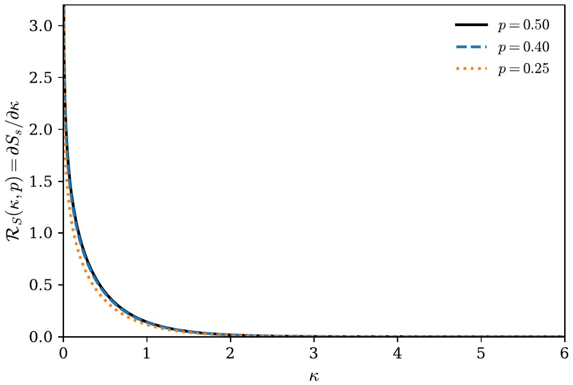
The response function is not introduced as an additional observable or as a new universal susceptibility. It is a local sensitivity measure within the Gaussian parametrization: at fixed p, R_s = ∂S_s/∂κ gives the change in entanglement entropy per unit change in the distinguishability coordinate κ. It therefore identifies the regime in which a small change in apparatus parameters or branch overlap produces the largest entropy change and makes the approach to saturation quantitatively explicit. The response is largest in the weak-distinguishability regime and decreases as the entropy approaches saturation. The corresponding time rate also depends on the apparatus-dependent factor dκ/dt. Because R_s is derived from S_s(κ,p), it contains no independent state information beyond the entropy law; its purpose is comparative sensitivity analysis. Figure 3 shows this response for several initial spin populations.

13. Universality Collapse Within the Gaussian Family

For a fixed input population p, different apparatus settings generate different functions κ_i(u). As a simple dimensionless example, let

$${\kappa }_i\left(u\right)=a_i{u}^2+b_i{u}^4,$$

(45)

which mirrors the momentum- and position-separation terms in Equation (37). The corresponding time-domain curves are

$$S_i\left(u\right)=S_s\left({\kappa }_i\left(u\right),p\right)$$

(46)

These curves need not coincide as functions of the time coordinate u. However, when each curve is replotted against its own κ_i, all curves obey the same fixed-p relation:

$$S_i=S_s\left(\kappa ,p\right)$$

(47)

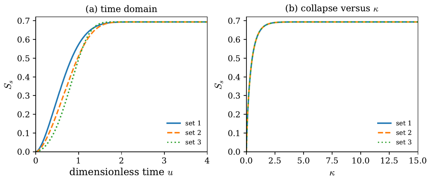
This is the operational meaning of the collapse: within the equal-width Gaussian family, the entropy retains no information about which parameter set produced a given value of κ. This statement does not imply a cross-family collapse for arbitrary non-Gaussian spatial states. Figure 4 illustrates the distinct time-domain trajectories and their collapse when replotted against κ.

14. Discussion

The conventional Stern–Gerlach picture emphasizes spatial separation. The overlap analysis shows that, for equal-width Gaussian branches, momentum separation also contributes to distinguishability before substantial spatial separation develops. In the constant-gradient example, the momentum contribution enters at order t², whereas the position contribution enters at order t⁴.

The central result should be understood at two levels. At the most general level considered here, the reduced-spin entropy of a pure two-branch state is completely determined by the pair (p,|γ|). This exact overlap statement is independent of Gaussianity. At the more specialized Gaussian level, the overlap magnitude can be represented by a coordinate κ, yielding S_s = S_s(κ,p). Free spreading and unequal widths do not invalidate the exact overlap law; they modify only the Gaussian expression used to compute the relevant overlap magnitude.

This distinction also separates closed-system spin–position entanglement from environmental decoherence. The entropy considered here is the entropy of a reduced subsystem of a globally pure state. Detector resolution, coarse-graining, thermal mixtures, and environmental coupling introduce additional physical mechanisms that require a more general model. Extending the present framework in these directions may help connect the overlap parametrization developed here to experimental readout and to broader decoherence models.

14.1. Representative Non-Gaussian Example

The distinction between the exact overlap law and the Gaussian phase-space reduction can be seen explicitly with a non-Gaussian packet. Consider normalized Laplace-shaped branches φ_j(x) = a^(−1/2) exp(−|x − x_j|/a) with equal mean momentum. Their overlap magnitude is |γ| = [1 + |Δx|/a] exp(−|Δx|/a), not exp(−κ) with the quadratic Gaussian coordinate of Equation (21). Nevertheless, once this non-Gaussian overlap is inserted into Equations (14) and (15), the reduced-spin spectrum and entropy are still determined exactly. This example makes explicit that the general result is the dependence on (p,|γ|), whereas the simple quadratic phase-space coordinate is a property of the chosen Gaussian family.

14.2. Experimental Access to the Entropy and Overlap Phase

The reduced-spin entropy can, in principle, be obtained without reconstructing the full spatial wave functions. Complete spin-state tomography measures the three Bloch components ⟨σx⟩, ⟨σy⟩, and ⟨σz⟩ and thereby reconstructs the 2 × 2 reduced density matrix ρ_s; its eigenvalues then give S_s directly. If the input coefficients c↑ and c↓ are known, the complex overlap can also be inferred from the off-diagonal element through γ = ρ↑↓/(c↑c↓*) up to the calibrated input spin phase. Spatial recombination is therefore not mathematically required to determine the reduced-spin entropy, although coherent recombination or interferometry provides a direct way to probe the phase arg γ and to verify retained branch coherence. Atom chip Stern–Gerlach splitting and complete Stern–Gerlach interferometry [16,17] provide natural experimental settings in which these ideas could be tested. In practice, state-tomography errors become most important near the weak-distinguishability limit because one eigenvalue of ρ_s is then very small.

14.3. Scope Beyond Ideal Linear Field and Spin-1/2

A physical magnetic field must satisfy Maxwell’s equation ∇·B = 0; so, the globally one-dimensional linear field used in the constant-gradient example is an effective local approximation to the relevant field component over a restricted region of the apparatus. In a full three-dimensional divergence-free field, transverse gradients and field curvature can modify the branch trajectories, widths, and shapes. The exact two-branch result of Section 4 does not depend on the linear-field approximation: whenever the final pure state can still be written as two spin branches, its reduced-spin entropy is determined by p and the actual overlap γ, which may be evaluated numerically. What generally fails outside the ideal Gaussian model is the simple closed form for κ(t), not the overlap law itself.

For spin larger than 1/2, a Stern–Gerlach interaction generally produces more than two spatial branches. Writing |Ψ⟩ = Σ_m c_m|m⟩|φ_m⟩ gives reduced-spin matrix elements (ρ_s)_mn = c_mc_n*⟨φ_n|φ_m⟩. The entropy then depends on the eigenvalues of this larger overlap-weighted matrix, or equivalently on the full Gram matrix of pairwise branch overlaps, and cannot, in general, be reduced to a single overlap magnitude. The spin-1/2 result should therefore be viewed as the simplest nontrivial member of a broader multi-branch structure.

15. Conclusions

We have derived the reduced-spin entropy generated by closed-system Stern–Gerlach spin–position entanglement and explicitly stated the domain of each reduction. For any normalized pure two-branch state, the reduced-spin spectrum and von Neumann entropy are exact functions of the initial spin population p and the branch-overlap magnitude |γ|. Equivalently, the distinguishability of the spatial branches may be expressed through the fidelity |γ|² or the trace distance D = √(1 − |γ|²). For equal-width, unchirped Gaussian branches, |γ| = exp(−κ), so the entropy can be parametrized by a Gaussian phase-space coordinate κ that combines relative position and momentum separation. Exact Heisenberg evolution under the linear Stern–Gerlach force justifies the displacement trajectories, while the covariance-based derivation for spreading packets accounts explicitly for the associated quadratic phase chirp. Freely spreading chirped Gaussians and unequal-width Gaussians modify the Gaussian expression for the overlap coordinate without altering the exact two-branch entropy law, and an explicit non-Gaussian example demonstrates that the general result survives when the quadratic Gaussian coordinate does not. The weak-distinguishability asymptotics, orthogonal-branch saturation, entropy response function, and fixed-population curve collapse all follow from this structure. The entropy can in principle be reconstructed by complete spin-state tomography, while the phase of the complex overlap can be accessed through the off-diagonal spin coherence or interferometric recombination. Beyond ideal linear fields, the branch overlap may require numerical evaluation, and higher-spin systems generally require a multi-branch overlap matrix rather than a single γ. The result is therefore not a shape-independent phase-space law for arbitrary Stern–Gerlach packets, but an exact two-branch overlap law supplemented by explicitly delimited Gaussian phase-space reductions.