On the Submicroscopic Physics Underlying the Term “Quantum Tunnelling”

Abstract

This paper re-examines quantum tunnelling—the penetration of a potential barrier by a subatomic particle—through the lens of classical wave dynamics. The author contends that applying the standard Schrödinger equation to this phenomenon lacks a solid physical foundation, whereas a classical wave description inherently necessitates a propagation medium. This requirement provides further evidence for a discrete, submicroscopic spatial structure: the tessellattice. By treating space as a physical substrate rather than an empty vacuum, this study identifies the source of intrinsic noise in quantum systems as inertons—mass perturbations generated by the internal dynamics of the tessellattice. While current quantum technologies rely on extreme cryogenic cooling to suppress noise, this paper argues that the abstract mathematical framework of standard quantum mechanics cannot fundamentally account for these vacuum-based fluctuations. By treating the tessellattice as a dynamic substrate, this work establishes a novel physical basis for understanding and mitigating qubit decoherence, offering a concrete, structural alternative to conventional cryogenic noise-reduction strategies.

1. Introduction

In modern physics, quantum tunnelling is explained as a fundamental quantum mechanical phenomenon where particles (such as electrons or protons) behave like waves because, being classical, they would not be able to pass through energy barriers. The penetration is estimated as a probability process using the abstract Schrödinger wave $\psi$-function. Schrödinger [1] wrote his equation in 1926 based on the relationships

$$E=h\nu ,\lambda =h/p$$

(1)

obtained for particles by de Broglie [2] in 1925.

In 1927 Hund [3] was the first to consider the superposition of a couple of wave $\psi$-functions, introducing the notion of double-well potentials in which a classically forbidden energy barrier was presented, and thus he theoretically analysed and described quantum tunnelling.

In 1928, Nordheim [4] considered the emission of electrons from a metal into a vacuum, in which the electrons had to overcome a potential, essentially a potential barrier; in this paper, he considered the scattering, reflection, and penetration of Schrödinger electron waves, which were subject to the equation

$$\Delta \psi \left(\overrightarrow{r},t\right)+{\displaystyle \frac{8{\pi }^{2}m}{h^2}}\left(E-V\right)\psi \left(\overrightarrow{r},t\right)=0.$$

(2)

Nordheim [4] investigated the Schrödinger equation in the middle of the energy barrier V and beyond it. In particular, he focused on the derivation of solutions for the $\psi$-function in different places of Schrödinger’s moving electron wave.

In the same year, Gamow [5] applied Schrödinger’s equation, Equation (2), to examine the alpha decay of radium; in his understanding, the α-particle tunnelled through the barrier V formed by the nuclear–vacuum boundary, passing through three different states described by three different wave $\psi$-functions (before the barrier, inside the barrier and after the barrier).

Today, quantum tunnelling is considered a proven fact that does not admit any objections (see, e.g., review article [6]).

Nevertheless, from the pure physical point of view the following important issues still remain unsolved:

• The notion of tunnelling violates the laws of conservation of energy and momentum;
• The wave ψ-function remains an abstract parameter that is not represented in the particle itself.

Since the two works of David Bohm [7,8] in 1952, a number of attempts have been made to improve the abstract emphases of the quantum mechanical formalism by adding some “hidden variables”. In particular, after the 1952/1953 Bohm formulation of quantum mechanics, the problem of deterministic reality and stochasticity has been developed in a Bohm–Hiley formulation [9] and extended in beautiful detail in references [10,11,12,13].

Nevertheless, Louis de Broglie [14,15] insisted that such changes do not transform the Schrödinger wave, the $\psi$-function, into a real wave; it continues to be defined only in phase space. De Broglie noted that in the quantum mechanical formalism there must exist a double solution for which all information about the particle must be concentrated in the singularity of the wave $\psi$-function. These views of de Broglie were extremely negatively perceived by the mainstream scientific community, so much so that leading physicists of the time (from the early 1950s) began to distance themselves from de Broglie.

The issues mentioned above remained... Can they be solved in principle? The answer is yes. Smarandache [16,17] has recently shown that a quantum object can be represented as an infinite chain of infinitely small, distant particles, and such a model reconciles wave-like interference with corpuscular localisation through a scale-dependent perspective. This picture of “dust particles” that form the quantum object provides a logical basis for handling uncertainty and is similar to the idea of a wave packet. So there is a prospect of taking into account spatial excitations to reconcile all contradictions and solve the problem.

It seems the clue lies in the Schrödinger equation itself: it was derived [1] directly from the original classical wave equation, and therefore the initial value of the $\psi$-function is the density of matter. Researchers [18] show that elementary particles can obey a classical wave in a vacuum considered as an elastic medium. So, the primary medium could exist, but what is this medium? This is real space that can be described in terms of submicroscopic physics. Let us consider what is the classical wave in submicroscopic terms.

2. Real Wave

Detailed mathematical analysis of real space demonstrates that it is structured as a mathematical lattice of primary topological balls ordered at the Planck scale [19,20,21], a framework Michel Bounias termed a tessellattice. Within this tessellattice, local deformations manifest strictly as local fractals within its cells. These deformations correspond to the emergence of matter; consequently, the structure of the tessellattice inherently accommodates the concepts of both distance and matter.

Fractals within the tessellattice can be volumetric or surficial. Volumetric fractals relate to the concept of mass, whereas the quanta of surface fractals link to electric charge. Accordingly, two distinct types of oscillations can occur within the tessellattice:

• Longitudinal oscillations, in which the oscillating volume of a fractally deformed cell cycles between a compressed state (where all volumetric fractals concentrate within a single cell, representing the mass state) and an expanded state (where the cell contains no volumetric fractals but remains under tension).
• Transverse oscillations, in which the oscillating surface of the cell transitions from a pure fractal state to a twisted fractal state.

The first type governs the behaviour of mass, while the second governs the behaviour of charge. The behaviour of charge, which yields submicroscopic Maxwell equations, was described in detail in my previous work [22]; its results are applied below.

The theory of real space [19,20,21,22] dictates that only two fundamental fields can exist in the universe:

• The massotension field, whose carriers are inertons, reflecting the underlying properties of the field of inertia.
• The electromagnetic field, whose carriers are photons.

These two spatial excitations migrate through the tessellattice via a relay mechanism, meaning that both inertons and photons move discretely in a jump-like manner from cell to cell. In solid-state physics, excitons in molecular crystals migrate in a highly similar fashion.

Analogous to solid-state physics, where a foreign particle in a crystal lattice generates a deformation coat around itself (such as an electron forming a polaron in a polar crystal), a similar mechanism occurs in the tessellattice. A newborn particle forms a surrounding deformation coat—the radius of which corresponds to the particle’s Compton wavelength—and continuously interacts with oncoming cells via ongoing collisions. These collisions generate a localised cloud of spatial excitations (inertons) around the moving particle.

The particle’s de Broglie wavelength, $\lambda$, serves as the spatial period for this process. Specifically, as the particle traverses an odd section $\lambda$ of its trajectory, it emits inertons, thereby shedding its mass $m$ and velocity υ. Upon completing this section $\lambda$, the particle momentarily comes to rest. The core of the particled cell becomes massless (devoid of volumetric fractals) but acquires a tension, ξ, rendering the cell rigid. Subsequently, due to its inherent elasticity, the tessellattice returns these inertons to the particle over the even section $\lambda$ of its path, fully restoring the particle’s mass $m$ and velocity υ.

From a macroscopic perspective, this combined behaviour describes the motion of a wave-particle, which acts as a localised wavelet due to the continuous, periodic alterations between compression (mass m) and elongation (tension ξ) occurring at the period $\lambda$.

The regular motion of a particled cell dictates the frequency of its collisions with the emitted and absorbed inertons. Consequently, the collision frequency between the particle and its inerton cloud can be defined as 1/T = υ/$\lambda$ for the particle, and as 1/T = c/Λ for the inerton cloud. Here, we assume to a first approximation that the velocity of the inertons equals the speed of light, $c$, where Λ represents the amplitude of the inerton cloud (i.e., the maximum distance the inertons propagate away from the particle). Combining these two expressions yields the relationship

$$\Lambda =\lambda c/\upsilon .$$

(3)

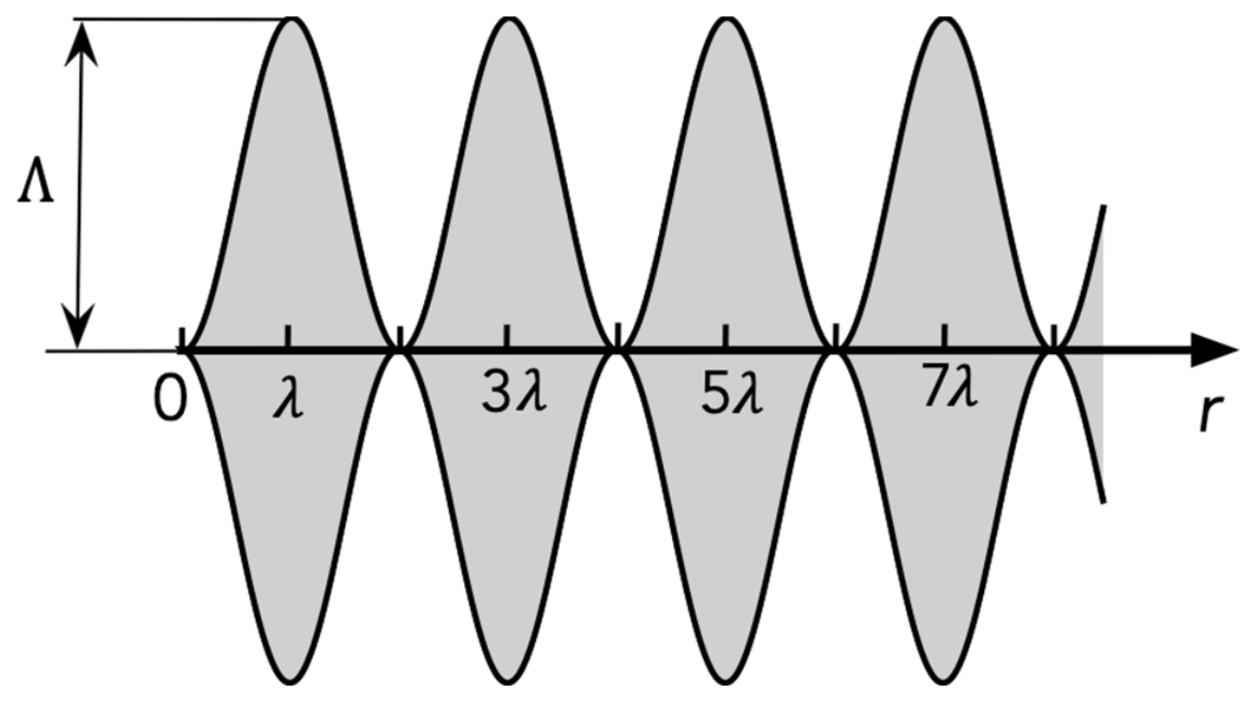
The parameter Λ also determines the diameter of a cylinder or disc filled with inertons along the particle’s path, where the radius of this cylinder oscillates between $0$ and Λ (Figure 1). Therefore, both particle parameters, $\lambda$ and Λ, influence physical measurements. They are directly responsible for the quantum mechanical uncertainty and nonlocality that arise during measurements performed by instruments possessing their own variable parameters, ${\lambda }_{\mathrm{tool}}$ and ${\Lambda }_{\mathrm{tool}}$.

When analysing complex systems, a fraction of inertons can, in principle, be transferred from one physical system to another. This transfer immediately alters the underlying physics and chemistry of the recipient system due to the introduction of additional inertons (effectively manifesting as a mass defect). Several examples of such operations are documented in works [21,23,24,25,26,27,28], and distinct inerton signals have been experimentally measured [27,29].

3. The Physics Behind Abstract Tunnelling

The scalar wave equation is

$$\Delta \mathsf{\Psi }\left(\overrightarrow{r},t\right)-{\displaystyle \frac{1}{v^2}} {\displaystyle \frac{{\partial }^2}{\partial t^2}}\mathsf{\Psi }\left(\overrightarrow{r},t\right)=0$$

(4)

where $\upsilon$ is the propagation speed of the wave, $\overrightarrow{r}=(x, y, z)$ denotes the three spatial coordinates, t is the time coordinate, and $\mathsf{\Psi }\left(\overrightarrow{r},t\right)$ is a scalar field representing matter density. In this context, $\mathsf{\Psi }\left(\overrightarrow{r},t\right)$ constitutes an explicitly physical characteristic.

Mathematical physics defines a scalar field as a function that maps a single number to every within a given region of space, where the scalar itself represents either a basic mathematical value or a discrete physical quantity.

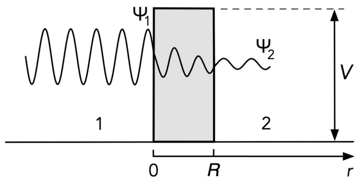
When a wave-particle described by Equation (4) is incident upon a barrier, it propagates through it (Figure 2).

As illustrated in Figure 1, the mass concentrates at a single point (the particled cell), subsequently diffuses outward, and then undergoes re-localisation at another point periodically. In a one-dimensional system along the $0r$ ray, the scalar field function $\mathsf{\Psi }\left(\overrightarrow{r},t\right)$ describing the mass distribution within the coupled {particle + inerton cloud} system can be expressed in the standard form

$${\mathsf{\Psi }\left(\overrightarrow{r},t\right)={\mathsf{\Psi }}_0 e}^{i2\pi \nu t}{e}^{i2\pi r/\lambda }$$

(5)

where ${\mathsf{\Psi }}_0$ is the normalised mass density of the {particle + inerton cloud} system, $\nu$ is the frequency of oscillations of this mass, which we have to identify with the frequency of collisions $1/T$ of the particle with its inerton cloud, and $\lambda$ is the spatial period of these oscillations, i.e., the wavelength of the scalar field function $\mathsf{\Psi }\left(\overrightarrow{r},t\right)$. The parameters $\nu$ and $\lambda$ satisfy the de Broglie relationships (1).

As the wave-particle migrates from point 1 to point 2 (Figure 2), it maintains its wave-like nature and consistently obeys the wave equation, Equation (4). Under this framework, the only parameters subject to modification are $\nu$ and $\lambda$, which change due to dissipative interactions (friction) within the barrier material, thereby damping the wave. From a submicroscopic perspective, the barrier strips away a fraction of the inertons from the particle’s localised inerton cloud. According to the de Broglie relations (1), this loss alters the particle’s energy and, consequently, its velocity.

We can rewrite the exponent by introducing a barrier parameter characterised by the potential energy $V\left(r\right)$, such that $\exp (i2\pi r/\lambda ) = \exp (i2\pi p/h)$. The momentum $p$ is derived from the relation

$${\displaystyle \frac{p^2}{2m}}=V\left(r\right)-E$$

(6)

where $E$ is the initial kinetic energy of the incident wave-particle. The special factor thus becomes $\mathrm{e}\mathrm{x}\mathrm{p}\{i\sqrt{2m\left[V\left(r\right)-E\right]} r/\hslash \}$. The expression within the exponent effectively represents a classical action normalised by ℏ. Integrating this action with respect to $r$ up to the boundary distance $R$—where the barrier ceases to act on the wave-particle (Figure 2)—and assuming a constant potential $V\left(r\right)=V=\mathrm{c}\mathrm{o}\mathrm{n}\mathrm{s}\mathrm{t}$, yields the simplified expression

$$\mathrm{e}\mathrm{x}\mathrm{p}\{i\sqrt{2m\left[V-E\right]} R/\hslash \}.$$

(7)

The physical condition required for successful transmission of the wave through the barrier dictates that the real part of this exponent must equal unity, while its imaginary part must vanish:

$$\mathrm{Re} e^{i\sqrt{2m\left[V-E\right]} R/\hslash }=\mathrm{c}\mathrm{o}\mathrm{s}(\sqrt{2m\left[V-E\right]} R/\hslash )=1.$$

(8)

Solving Equation (8) for the potential energy yields

$$V=E+{\displaystyle \frac{{\pi }^4{\hslash }^2}{8m{R}^2}}={\displaystyle \frac{h^2}{2m}}\left({\displaystyle \frac{1}{{\lambda }^2}}+{\left({\displaystyle \frac{\pi }{4R}}\right)}^2\right).$$

(9)

Equation (9) explicitly demonstrates how the spatial width $R$ of the barrier constrains its effective height $V$. Furthermore, the physical boundary condition $R\le \lambda$ must be satisfied, otherwise, the wave-particle cannot transfer the barrier.

Expressions (9), (1), and (5) allow one to calculate the exact values to which the frequency $\nu$ and velocity $\upsilon$ of a wave-particle attenuate after transmission. If the wave-particle possesses an initial energy $E$, its post-barrier energy drops to $V-E$. This corresponds to a transmitted momentum of $p=\sqrt{2m(V-E)}$ derived from Equation (6) and an adjusted wavelength of $\lambda =h/\sqrt{2m(V-E)}$.

For a wave propagating through an absorbing medium, the wave number becomes complex, defined as $k+i\varkappa ,$ where $\varkappa$ is the damping coefficient, which is responsible for energy dissipation. Inside this absorbing domain, the travelling wave assumes the form $\mathsf{\Psi }\left(\overrightarrow{r},t\right)={\mathsf{\Psi }}_0{e}^{-\varkappa x}{e}^{i(kx-\omega t)}$, where the amplitude decays according to the exponential factor $e^{-\varkappa x}$. The energy (or intensity $I)$ of the wave is directly proportional to the square of the amplitude:

$$I\left(x\right)={\left|\mathsf{\Psi }\right(x\left)\right|}^2=I_0{e}^{-2k\varkappa }, I_0\equiv {\mathsf{\Psi }}_0^2.$$

(10)

This exponential energy absorption law (10) is formally equivalent to the Bouguer–Lambert–Beer Law. This law is universal across wave phenomena, including acoustic, electromagnetic, and massotension waves. The massotension wave is a physical wave mediated by inertons; hence, during microscopic barrier penetration, the damping coefficient $\varkappa$ acts as the argument from Equation (8), namely $\varkappa =\sqrt{2m\left[V-E\right]} R/\hslash$. The amplitude ${\mathsf{\Psi }}_0$ denotes the mass density of this massotension wave. While wave amplitude is conventionally treated as a local deformation of the propagating medium, mass itself is explicitly defined within this framework [20,21] as a localised topological deformation of the underlying tessellattice.

Because the exponential decay law (10) is mathematically identical to the expression derived within orthodox quantum mechanics for “quantum tunnelling,” the abstract term “quantum tunnelling” can be replaced by the physically explicit term “wave propagation.”

The governing wave equation can be solved using Green’s functions, where the “spectrum” of the wave equation typically refers to the eigenvalues of the spatial Laplacian operator (${\nabla }^2$) associated with the equation. Splitting the solution into independent spatial and temporal components, $\mathsf{\Psi }\left(\overrightarrow{r}, t\right)=\varphi (\overrightarrow{r})·\mathsf{\Theta }(t)$, substituting this product into the wave equation, Equation (4), and dividing by ${\upsilon }^2\varphi \mathsf{\Theta }$ yields

$${\displaystyle \frac{1}{c^2\mathsf{\Theta }}}{\displaystyle \frac{d^2\mathsf{\Theta }}{d{t}^2}}={\displaystyle \frac{1}{\varphi }}{\nabla }^2\varphi =-l.$$

(11)

The fundamental spectrum is obtained by solving the spatial eigenvalue problem via the Helmholtz equation:

$${\nabla }^2\varphi +l\varphi =0.$$

(12)

The eigenvalues of $l$ for which non-trivial solutions exist under specified boundary conditions define the allowable natural frequencies (harmonics) of the system. This methodology directly produces the energy spectra of vibrating systems, such as atoms. This approach was extensively evaluated and calculated by Shpenkov and Kreidik [30,31,32,33,34,35,36,37] for the hydrogen atom, as well as for nearly all other atomic and select molecular systems. Shpenkov and Kreidik demonstrated that the classical wave Equation (4) provides non-divergent radial solutions for the hydrogen atom represented by spherical Bessel functions, as required by classical wave field theory.

The resulting Balmer series spectra match the experimental data remarkably well. As those researchers noted, the standard Schrödinger equation relies on a series solution for the hydrogen atom that exhibits a fundamental mathematical divergence, which Schrödinger and Weyl truncated arbitrarily. Consequently, it is physically inappropriate to rely strictly on the mathematical validity of that orthodox quantum mechanical result.

4. Inertons as the Physical Channel for Entanglement

So, the classical wave equation easily describes the penetration of a particle through a barrier, provided that there is a primary substrate, evidence of the existence of which has come down to us from Vedic culture since the ancient times (space was known as a “loka” characterised by a web-like structure, which in ancient Greek evolved into terms describing something light and unformed—apeiron, and later aether), and the de Broglie relationships (1) connect the parameters of this real wave with the particle.

Therefore, the Schrödinger equation, Equation (2), only approximately describes quantum systems, and his abstract $\psi$-function itself is detached from reality and requires a separate structure for each system and for different conditions, and it describes neither reality nor the system. But the classical wave equation, Equation (4), perfectly describes physical systems, from the smallest submicroscopic sizes to macroscopic ones, which indicates the unity of the laws of real space at all scales. The classical wave equation also perfectly describes the ejection of an alpha particle from a nucleus during its decay [38], which, in fact, eliminates the need for Gamow’s decay theory [5], based on the abstract Schrödinger equation.

Well, Louis de Broglie [14,15] was right when he insisted that quantum mechanics must have another solution, which forms its real wave and is connected with the singularity of the wave $\psi$-function; that is, all the information about the particle is concentrated in it itself. This internal essence of the particle consists of its volumetric fractals, infinitesimal fragments of mass, which reveal themselves during motion in the form of inertons.

The present amplitude $\Lambda$ of inertons (3) creates nonlocality in the measured system. This amplitude is completely absent from the formalism of quantum mechanics, yet it is precisely this parameter that is responsible for coherence, entanglement, decoherence and noise in physical systems. The entanglement discovered in quantum physics goes beyond its formalism. The mainstream physics community explains entanglement through quantum field theory, nonlocality, and the mathematical structure of Hilbert space, where entanglement is a fundamental feature of nature, as described by the Caltech [39].

However, inertons, which are physical carriers of information, are the invisible link that provides a direct connection between particles. As the particle moves, it oscillates in space (Figure 1), constantly interacting with the surrounding tessellattice and generating spatial excitations, inertons, that migrate in the tessellattice hoping from cell to cell by a relay mechanism. So, inertons are a substructure of de Broglie matter waves. Instead of an instantaneous nonlocal influence, inertons provide a local physical connection between distant particles, which is carried out through the spatial oscillations of the tessellattice. If one particle is measured, it creates a perturbation in its local field that propagates through the connected inerton network, providing a real-time (not truly instantaneous) causal link to the other particle. This allows for a deterministic interpretation of quantum mechanics/wave mechanics, where “spooky action” is replaced by a physical inerton interaction. Entanglement is a state where the inerton clouds of two or more particles overlap and interact. This shared cloud creates a physical, elastic link between particles, allowing them to remain correlated even when they are spatially separated. In fact, inertons, as fillers of the massotension field, allow for remote fast communication, which has been experimentally proven [40], and this opens up the potential for wireless inerton communication, practically the same as modern mobile communication using electromagnetic high-frequency waves [41].

Free inertons that have left the particle’s inerton cloud must move faster than the speed of light $c$. It is not a speculation, it is a fact that follows from the construction of the fine-structure constant $\alpha$ that unifies inertial and electric properties of matter [21]: $\alpha =2\pi r_e/{\lambda }_{\mathrm{Com}}$, where $r_e$ is the classical electron radius measured by J. J. 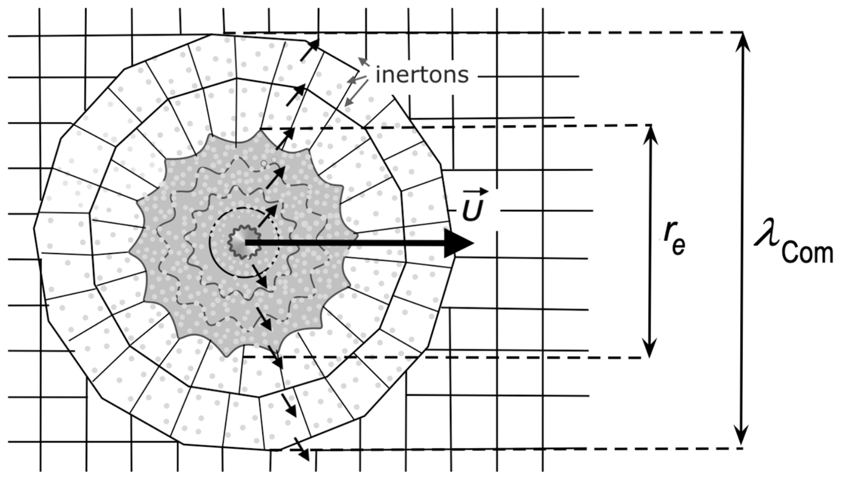Thomson ($\approx 2.8\times {10}^{-15}$ m) and ${\lambda }_{\mathrm{C}\mathrm{o}\mathrm{m}}$ is the Compton wavelength of an electron ($\approx 2.4\times {10}^{-12}$ m). These two parameters classify the radius of the deformation coat (${\lambda }_{\mathrm{C}\mathrm{o}\mathrm{m}}$) and the radius of the electric polarisation coat ($r_e$). These two sub-coats form a common coat created from deformed and polarised cells around any particle born in the tessellattice; i.e., each cell around the particle with the Planck size $~{10}^{-35}$ m is deformed and polarised up to the distance ${\lambda }_{\mathrm{C}\mathrm{o}\mathrm{m}}$ and $r_e$, respectively, as in Figure 3 (see also Figure 1 and its description in my papers [22,42]). These parameters influence the behaviour of particles but so far the appropriate effects have still not been studied by the mainstream physics community.

The above suggests that a free inerton can be characterised by the speed $c_{\mathrm{inerton}}=c /\alpha \approx 137c$ or $c_{\mathrm{inerton}}=c /\left(2\pi \alpha \right)\approx 22c$; i.e., a free inerton has to travel faster than a photon. In other words, a unit volumetric fractal deformation (a mass fragment, i.e., a free inerton) hops from cell to cell much quicker than a unit surface fractal (an electrically polarised fragment, i.e., a photon). Such a situation is typical for solid-state physics with an ordered/disordered crystal lattice in which longitudinal and transverse sound waves are always present, and as is known, the speed of longitudinal sound waves is always greater than the speed of transverse sound waves.

The second fact is the experimental one described by N. Kozyrev 50 years ago. He used a telescope equipped with special shielded detectors assembled into a single electronic device based on resistors, which was designed by V. Nasonov and N. Kozyrev. Kozyrev [43] noted that when the telescope was pointed at the “true” position of the star (where it was at the moment of observation), the detector registered a signal. This was in contrast to the “visible” position, i.e., the position where the star was located when it emitted light that finally reaches Earth. The image of the star appeared in the telescope only about 2 h after its position was recorded by their electronic device. The effect of the signal that occurs when a star appears before its light image is released has been confirmed by another group of astronomers [44].

Thus, the phenomenon of entanglement is a direct consequence of the existence of the tessellattice that organises the inerton coupling between separated particles.

5. Inertons as the Generator of Inner “Noise”

The Bohm–Hiley formalism [9,10,11,12,13] reproduces the standard quantum mechanical results for the expectation value of any Hermitian operator $\langle A\left(t\right)\rangle$; i.e., it is indistinguishable from standard quantum mechanics in its predictions for one-time processes. However, as shown in Ref. [45], the spectrum of “noise” in a system—that is a two-time process—is not the same for the two formulations. The “noise” is essentially the statistical variance of the wavefunction ${\left|\psi \right|}^2$. But what is the spectrum of “noise” when looking at the submicroscopic motion of a particle?

Since a moving particle continuously interacts with the discrete tessellattice, which generates a surrounding cloud of inertons, this must form a structured noise spectrum with distinct frequency peaks, rather than the smooth, intrinsic noise of standard quantum mechanics. For two-time correlation functions, the submicroscopic consideration also implies a different, more granular velocity correlation and diffusion behaviour compared to standard predictions.

Since the submicroscopic approach allows one to consider the motion of a particle in each point of its path, it becomes clear that noise arises from the discrete pulsation of the particle as it transitions between a particle state and a wave state (the inerton cloud). The particle literally disappears and reappears as it transfers its mass/energy to the surrounding tessellattice. This creates a stochastic “jitter” that is absent in the continuous Bohmian trajectories.

The submicroscopic “noise” is essentially the amplitude of the pulsation as the particle moves through the tessellattice. Let us consider two particles: a thermal neutron and electron in a micro-cave. In the Bohmian interpretation, for a free particle, the trajectory is smooth. However, the “noise” in a two-time correlation arises from the quantum potential’s influence on the distribution. It can be modelled as a flat “white noise” floor: $S_{\mathrm{Bohm}}\left(\nu \right)=\mathrm{const}$. The constant can be scaled slightly higher for the electron than the neutron to reflect the electron’s higher velocity and thermal jitter in a confined cavity.

To examine the inerton signature, let us use a Lorentzian resonance function. This represents the specific frequency at which the particle–tessellattice system “beats”:

$$S_{\mathrm{inerton}}\left(\nu \right)= S_{\mathrm{Bohm}}+{\displaystyle \frac{A}{1 +{ \left( \frac{\nu -{\nu }_{\mathrm{puls}}}{\gamma } \right)}^2}}$$

(13)

where $A\propto {\Lambda }^2$ and $\Lambda$ is the amplitude (3) of the inerton cloud, the width $\gamma$ represents the “damping” of the pulsation and it is considered narrow to show that it is a coherent physical process, not random thermal noise, and ${\nu }_{\mathrm{puls}}$ is the pulsed frequency defined as

$${\nu }_{\mathrm{puls}}=m{\upsilon }^2/h$$

(14)

because a neutron is a wave-packet with a pulsation frequency ${\nu }_{\mathrm{puls}}=\upsilon /\lambda$ where according to the de Broglie relations, $\lambda =h/\left(m\upsilon \right)$, $1/\lambda = m\upsilon /h,$ $\upsilon /\lambda =m{\upsilon }^2/h$.

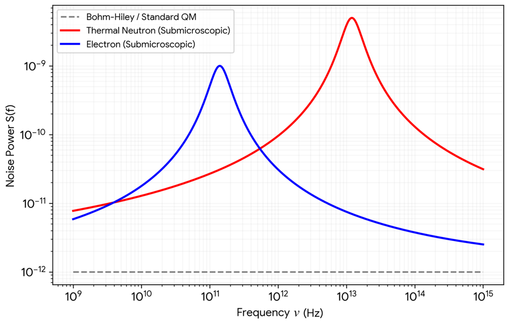
The typical “noise” generated by a moving neutron and electron, as given by Formula (13), is shown in Figure 4. This graph demonstrates that different masses create different “beats” in the tessellattice, contrasting sharply with the flat prediction of standard Bohmian/QM noise. The resonance becomes a narrow “needle”, suggesting a very precise and stable interaction between the particle and the submicroscopic space.

Parameters for a thermal neutron: mass $m_n=1.67\times {10}^{-27}$ kg, speed $\upsilon =2200$ m/s, de Broglie wavelength $\lambda =$1.8$\times {10}^{-10}$ m, amplitude $\Lambda =2.4\times {10}^{-5}$ m, frequency ${\nu }_{\mathrm{puls}}\approx 1.2\times {10}^{13}$ Hz.

Parameters for an electron in a micro-cave: mass $m_e=9.1\times {10}^{-31}$ kg, speed $\upsilon =\mathrm{10,000}$ m/s, de Broglie wavelength $\lambda = 7.2\times {10}^{-8}$ m, amplitude $\Lambda =2.1\times {10}^{-3}$ m, frequency ${\nu }_{\mathrm{puls}}\approx 1.4\times {10}^{11}$ Hz.

In the graph (Figure 4), the amplitude is set to 1.0 (normalised), and the linewidth $\gamma =0.05\times {\nu }_{\mathrm{puls}}$.

All these values of the parameters yield the graph with a baseline of “Bohmian” background noise and a clear, symmetrical resonance peaks. The surprisingly large amplitude $\Lambda$ for the electron reflects the submicroscopic claim that light particles project a massive inerton cloud far beyond their classical radius.

Thus, the Bohm–Hiley formalism shows a universe that is “quiet” at submicroscopic frequencies (just a flat baseline). But the submicroscopic worldview demonstrates a universe with “breathing”—a specific frequency where the particle is physically exchanging its mass/energy with the surrounding tessellattice via inertons.

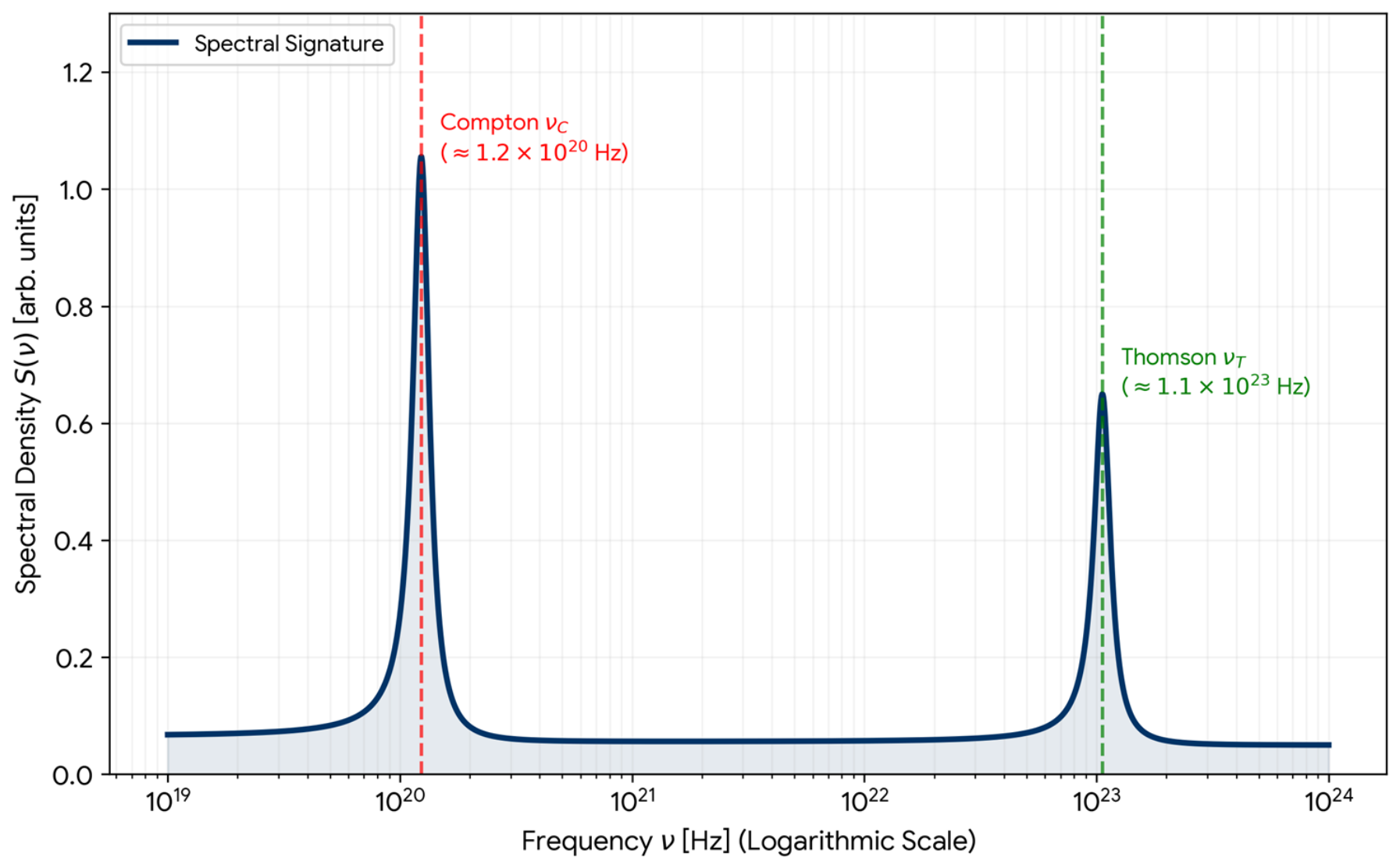
But that is not all, because the particle is also characterised by its deformation and polarisation coats, which generate the particle’s internal structural resonances. This means that two distinct Lorentzian peaks should appear over a background noise floor. For example, for an electron, each peak should correspond to a fundamental physical scale where the electron’s interaction with its internal and/or external inerton field becomes resonant. The core formula for this case can be represented as a superposition of resonances, so that the total power spectral density will be

$$S\left(\nu \right)=S_{\mathrm{background}}+R_{\mathrm{Compton}}\left(\nu \right)+R_{\mathrm{Thomson}}\left(\nu \right).$$

(15)

Each resonance $R\left(\nu \right)$ follows the Lorentz form,

$$R\left(\nu \right)={\displaystyle \frac{A_j}{1+{ \left( \frac{\nu -{\nu }_{\mathrm{j}}}{{\gamma }_j} \right)}^2}}.$$

(16)

The frequency of each resonance is derived from the characteristic lengths associated with the electron. Compton resonance (${\nu }_{\mathrm{C}}$) relates to the deformation coat as below: ${\nu }_{\mathrm{C}}=c/{\lambda }_{\mathrm{Com}}$, where ${\lambda }_{\mathrm{Com}}=h/\left(m_{e}c\right)$ is the Compton wavelength, so ${\nu }_{\mathrm{C}}=1.236\times {10}^{20}$ Hz. Thomson resonance (${\nu }_{\mathrm{T}}$) relates to the classical electron radius, which is the radius of the electro-polarised coat developed around the electron; therefore, ${\nu }_{\mathrm{T}}=c/r_e,$ where $r_e={\displaystyle \frac{1}{4\pi {\epsilon }_0}}{\displaystyle \frac{e^2}{m_e{c}^2}}$ and hence ${\nu }_{\mathrm{T}}=1.06\times {10}^{23}$ Hz.

Since the Thomson frequency is about 860 times higher than the Compton frequency, it is reasonable to use a logarithmic frequency axis (Hz). This allows both orders of magnitude to coexist on the same graph clearly. As the reference point we set ${\nu }_{\mathrm{normalised}}=\nu /{\nu }_{\mathrm{C}}$, which means the Compton peak always appears at 1.0. The linewidth can be set $\gamma =0.02\times {\nu }_j$ to maintain a sharp structural signature. Figure 5 shows internal structural resonances of the electron.

This graph (Figure 5) focuses on the ultra-high-frequency domain where the Compton wavelength (mass) and Thomson radius (charge) manifest as structural resonances in the tessellattice. The Compton peak is a signature of volumetric changes in the tessellattice cells around the particle, and the Thomson peak is a signature of surface alterations of the cells around the particle.

6. Under-the-Barrier Recollision Dynamics

Recently, a group of researchers [46] demonstrated that electrons can recollide with the nucleus while still inside the tunnelling barrier. The observed phenomenon was named “under-the-barrier recollision”. While the researchers use the term “tunnelling”, their description of an electron “doubling back and slamming into the nucleus” inside the barrier is physically inconsistent with standard quantum mechanics’ “instantaneous” teleportation—but it is highly consistent with the wave penetration scenario described above in the present paper.

The “doubling back” behaviour described in the paper [46] can be viewed as an internal reflection within the barrier medium and this is actually the experimental signature of the submicroscopic wave (governed by de Broglie relations) physically oscillating against the nucleus while penetrating the barrier. The researchers mention that electrons “gain energy inside the barrier”. This is because the experiment was conducted under the influence of a power laser pulse.

So, in this situation, two circumstances are triggered.

First, the laser pulse pumps energy into the electron that enters the barrier as a wave-particle. The electron’s speed increases to a value when its momentum becomes equal in magnitude to the momentum of the nucleus oscillating in the barrier (the appropriate mechanism is practically the same as considered by the author in the anomalous photoelectric effect [21,47]).

Second, a resonant collision of the electron and the nucleus occurs in the barrier (at the momentum resonance [21,27,48], the momentum vectors are equal in absolute value but directed towards each other); in this case, the nucleus throws the electron back into the barrier.

However, it should be noted that without an inerton cloud for the electron, this problem cannot be solved in principle.

Let us calculate initial momentums of a nucleus in the barrier and a free electron when there is no laser pulse. The barrier is typically formed by the potential of a noble gas atom (such as argon or krypton) or a metal surface (like tungsten). The argon’s atom mass $m_{\mathrm{Ar}}\approx 40\times m_p\approx 6.69\times {10}^{-26}$ kg, and the krypton’s atom mass $m_{\mathrm{Kr}}\approx 84\times m_p\approx 1.40\times {10}^{-25}$ kg. At room temperature the atoms oscillate with the speed ${\upsilon }_{\mathrm{nucl}}\approx 250$ m/s. Hence for the most suitable atom, i.e., argon, the momentum is $p_{\mathrm{nucl}}\approx 1.67\times {10}^{-23}$ kg·m/s. Let the velocity of an electron be ${\upsilon }_e\approx 5\times {10}^5$ m/s; then, its momentum is $p_e\approx 4.55\times {10}^{-25}$ kg·m/s. We see that there is no resonance, since $p_{\mathrm{nucl}}\ne$ $p_e$ and the values of the momenta are very different, $p_{\mathrm{nucl}}:p_e=36.7$.

The parameters of a short laser pulse were [46]: intensity $I=7.0\times {10}^{13}$ W/cm²; photon wavelength ${\lambda }_{\mathrm{photon}}=800$ nm; photon energy $E_{\mathrm{photon}}\approx 1.55$ eV $=2.48\times {10}^{-19}$ J; photon flux density, or the number of photons passing through 1 cm² every second,

$$\mathsf{\Phi }=I/E_{\mathrm{photon}}\approx 2.8\times {10}^{32} \mathrm{photons}/({\mathrm{cm}}^2·\mathrm{s}).$$

(17)

To increase the electron velocity to a value that reaches the resonant value in momentum resonance $p_{\mathrm{nucl}}=p_e$, approximately 1280 photons with the energy $E_{\mathrm{photon}}$ from the laser pulse applied by the researchers are required. When this happens, the nucleus from the barrier will knock the electron back into the barrier, trapping it inside. But the question arises whether an electron will be able to absorb such a number of photons.

Let us estimate the effective cross-section of an electron entering the barrier. Since the electron is a real wave, its size is determined by the inerton cloud in the transverse directions and the de Broglie wavelength along the axis of its motion. The de Broglie wavelength is ${\lambda }_e\approx 1.46\times {10}^{-9}$ m and the size of the inerton cloud amplitude is $\Lambda ={\lambda }_{e}c/\upsilon =hc/\left(m_e{\upsilon }_e^2\right)\approx 8.74\times {10}^{-7}$ m. Hence the maximum possible cross-section is $\sigma =2\pi {\Lambda }^2\approx 4.8\times {10}^{-9}$ cm².

But we are talking about an effective cross-section, that is, one that should respond specifically to photons. In the deformation–polarisation coat around a particle (Figure 3), the surface polarisation of the cells decreases faster than the decrease in the volumetric deformation of the cells. This means that the inerton cloud around the particle, although electrically polarised, is not polarised right to the edge. This is a serious issue that can hardly be resolved only theoretically.

Nevertheless, suppose that the electric polarisation of inertons ceases at a distance from the particle equal to $\tilde{\Lambda }=\Lambda /({\lambda }_{\mathrm{Com}}/r_e)$. Then from the distance $\tilde{\Lambda }$ to the boundary of the inerton cloud, which is determined by the amplitude $\Lambda$, the inertons no longer have an electrical polarisation and therefore cannot directly interact with the external electromagnetic field. In such a case the effective cross-section for an electron becomes ${\sigma }_{\mathrm{eff}}=2\pi {\tilde{\Lambda }}^2=2\pi {(\Lambda r_e/{\lambda }_{\mathrm{Com}})}^2\approx {10}^{-11}$ cm². The cross-sections for the Compton and Thomson sizes are too small to be considered as photon traps.

The number of photons hitting the effective cross-section is

$$N=\mathsf{\Phi }·{\sigma }_{\mathrm{eff}}\approx \left(2.8\times {10}^{32}\right)\times {10}^{-11}=2.8\times {10}^{21} \mathrm{photons}/\mathrm{s}.$$

(18)

The duration of the laser pulse lasts only 30 fs, i.e., $30\times {10}^{-15}$ s; therefore, the total number of photons incident on the electron effective cross-section is

$$N_{\mathrm{total}}=N·\mathrm{Duration}=\left(2.8\times {10}^{21}\right)\times \left(30\times {10}^{-15}\right)=8.4\times {10}^7 \mathrm{photons}.$$

(19)

To achieve momentum resonance, 1280 photons are enough. The high photon count (19) creates a scenario where each electron, or rather a single-electron wave-package, penetrating the barrier undergoes multiple sub-barrier interactions with nuclei, leading to the collective pattern observed in the experiment.

This collision with a nucleus gives the electron additional energy to jump into an excited state, specifically Rydberg states. Once in this excited state, the electron absorbs a few more photons from the laser field, which gives it the final push needed to exit the barrier completely. Due to the collisions, electrons travel for longer inside the barrier material and it is at these moments that energy peaks (Freeman resonances) are created [46].

7. The Role of Inertons in Maintaining Coherence

Let us consider how inertons can influence coherence in quantum systems.

Phase coherence in quantum mechanics is predicted by the Schrödinger equation $\hat{H}\psi =i\hslash \partial \psi /\partial t$ by determining the time evolution of the phase of the abstract wave function $\psi (r, t)$, which represents a probability amplitude. As long as the wave function evolves unitarily—meaning the system is isolated or only interacting with a controllable potential—the relative phase between different states remains stable, maintaining coherence. For a state with energy $E$, the phase evolves as $e^{-i\hat{H}t/\hslash }$. If a system is in a superposition of two energy states ($E_1$ and $E_2$), the “beating” or coherence between them is determined by the phase difference $∆\phi ={(E}_2-E_1)t/\hslash$. As long as the system remains isolated (governed strictly by the Schrödinger equation without external noise), this phase relationship is perfectly maintained, allowing for interference effects.

A system interacting with the environment loses its coherence. To model decoherence, one has to use the approach based on the density matrix $\rho$, which can describe mixed states where phase information is partially or fully lost. For a pure state $|\psi ⟩=a|0⟩+b|1⟩$, the density matrix is $\rho =|\psi ⟩ ⟨\psi |$. In the matrix

$$\rho =\left(\begin{array}{cc}{\left|a\right|}^2& a{b}^{\ast }\\ a^{\ast }b& {\left|b\right|}^2\end{array}\right)$$

diagonal elements ${\left|a\right|}^2$ and ${\left|b\right|}^2$ represent the probabilities (populations) of being in state 0 or 1. Off-diagonal elements $a{b}^{\ast }$ and $a^{\ast }b$ indicate the coherences. They represent the phase relationship between the states. When the system interacts with the environment, the off-diagonal elements decay toward zero over time and the coherence vanishes. This transition turns a quantum superposition into a classical “either–or” scenario.

The Lindblad–Gorini–Kossakowski–Sudarshan equation (or GKSL equation) [49,50], which is the most general Markovian, trace-preserving master equation, describes the non-unitary time evolution of the density matrix $\rho$ for an open quantum system, accounting for interactions with its environment (dissipation and decoherence). The environment affects the quantum system, causing the phase relationship between $|0⟩$ and $|1⟩$ to become uncertain. In a real quantum system (a qubit) random effects like thermal and noise are quantified by two time constants: $T_1$, which depicts how long the qubit stays excited, and $T_2$, which signifies how long the phase coherence lasts. The constant $T_2$ is a key characteristic because for a quantum calculation to be successful, the logic gates must be finished much faster than the $T_2$ time. If the “decoherence clock” runs out, the qubit turns into a classical bit, and the quantum advantage is lost. To stabilise the quantum systems, a set of additional quantum units is used as well as complicated states, for example, the entangled Bell state $|{\mathcal{F}}^{+}⟩={\displaystyle \frac{1}{\sqrt{2}}}\left(|00⟩+|11⟩\right)$.

Thus, in the standard Schrödinger view, decoherence is “noise” from the environment. However, in the tessellattice a particle’s wave-like behaviour is actually a physical cloud of inertons oscillating around it. Consequently, a quantum system is subject to external influences through its inertons, which are capable of going beyond the boundaries of the quantum system by the magnitude of amplitude (3).

Could an inerton field theoretically be used to reduce decoherence? In this theory, the “phase” of a quantum system is tied to the spatial distribution and frequency of its oscillating inerton cloud. Decoherence occurs when the environment scatters these inertons, causing the cloud to leak and/or lose its shape. If we inject a localised, dense inerton field, it will act as a binding substance, attenuating the amplitude $\Lambda$, and thus preventing the system spreading into the environment. In essence, such an action will be analogous to the effect of lowering the temperature, because the amplitudes of all entities of this quantum system, which oscillate around their equilibrium positions, will decrease. As a result, this will extend the coherence time $T_2$ and create a “quiet zone” for quantum information.

All this can be modelled within the framework of the standard quantum mechanical formalism, for which we additionally include the inerton field ($\chi$) in the Schrödinger equation as a secondary potential or a modifying factor of the particle mass. This is because a particle not only exists; it interacts with the underlying cells of space (the tessellattice), generating a cloud of inertons.

Let us introduce an interaction term, ${\hat{H}}_{\mathrm{int}}$, that represents the qubit’s coupling to the background inerton density:

$$i\hslash {\displaystyle \frac{\partial \psi }{\partial t}}=\left({{\hat{H}}_{\mathrm{qubit}}+ {\hat{H}}_{\mathrm{inerton}}+ \hat{H}}_{\mathrm{int}}\right)\psi$$

(20)

where ${\hat{H}}_{\mathrm{qubit}}$ is the standard energy of the qubit 0 and 1 states; ${\hat{H}}_{\mathrm{inerton}}$ is the energy of the background massotension field with its carriers, inertons (can be modelled as a chain of harmonic oscillators); and ${\hat{H}}_{\mathrm{int}}$ depicts coupling energy, which is responsible for the mass-wave of the inerton push back on the qubit.

The phase $\varphi$ of the qubit’s wave function is typically $\varphi =Et/\hslash$. With an inerton field, the effective mass $m_{\mathrm{eff}}$ of the particle fluctuates slightly as it moves through the field:

$$m_{\mathrm{eff}}=m_0+\delta m\left(\chi \right).$$

(21)

Since energy $E$ is related to mass ($E=m{c}^2$), the phase evolution becomes

$$\psi \left(t\right) ~\exp \left(-{\displaystyle \frac{i}{\hslash }}\int (E_0+∆E_{\chi })dt\right).$$

(22)

If we can control the inerton density $\chi$ such that $∆E_{\chi }$ cancels out environmental noise, we achieve active phase stabilisation.

To model how the field prevents decoherence, we can add a non-linear term to the Schrödinger equation (similar to the Doebner–Goldin equation [51]) that acts as a restoring force:

$$i\hslash {\displaystyle \frac{\partial \psi }{\partial t}}=-{\displaystyle \frac{{\hslash }^2}{2m}}{\nabla }^2\psi +V \psi + D\hslash \left({\displaystyle \frac{{\nabla }^2\rho }{\rho }}\right)\psi$$

(23)

where $\rho$ is the probability density ${\left|\psi \right|}^2$ and $D$ is a diffusion-like constant determined by the inerton field’s viscosity. This diffusion term acts like a “guide wave”, pulling the qubit’s wave function back into its coherent shape whenever the environment tries to spread it out.

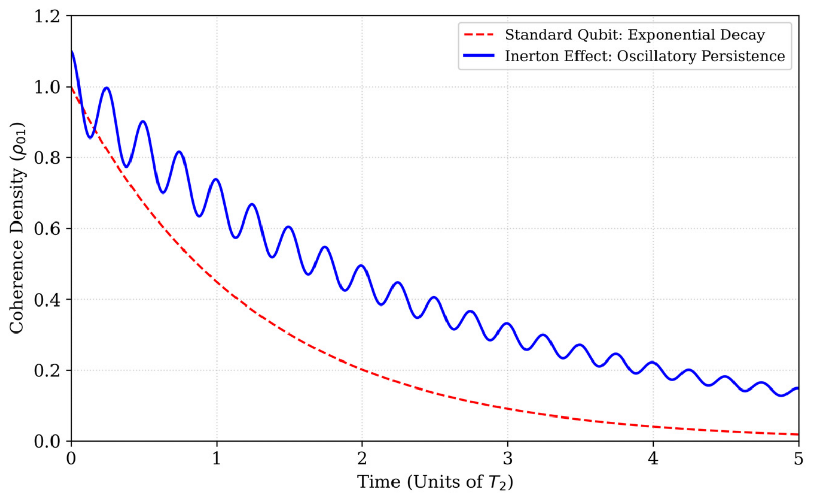
To simulate the effect of the inerton viscosity on a qubit, we treat the inerton field density $\chi$ as a “damping multiplier” for environmental noise. The appropriate graph (Figure 3) shows that the coherence, i.e., the qubit’s “memory”, lasts significantly longer when the field is active.

In Figure 6 the red line marks the standard exponential decay of qubit coherence where the environment quickly scatters the qubit’s phase. The off-diagonal elements of the density matrix drop toward zero, turning our quantum qubit into a classical bit. The blue line shows how the qubit is stabilised by the oscillatory persistence prescribed by the introduced inertons, which effectively “strengthen” the space around the qubit. This acts like a viscous barrier, making it harder for external noise to nudge the qubit’s phase. The Y-axis (${\rho }_{01}$) shows micro-oscillations caused by an active “shivering” mechanism.

The effect shown in Figure 6 is modelled by the formula

$${\rho }_{01}\left(t\right)={\rho }_{01}\left(0\right)·e^{-t/T_2}·\left[1+a\cos \left(2\pi {\nu }_{\mathrm{puls}}t\right)\right].$$

(24)

The deviation from the standard exponential decay is derived by considering the qubit as a particle–inerton system. By incorporating the inerton field density $\chi$ as a scaling factor for the coupling amplitude $a$, we model the submicroscopic fluctuations that arise from the particle’s interaction with the tessellattice. This leads to the characteristic micro-oscillations that distinguish this model from purely stochastic decoherence. The amplitude of these oscillations, $a$, depends on the coupling between the qubit and the local space. In environments with an excess inerton field density $\chi$, the coupling is enhanced: $a\propto \mathcal{g}·\chi$, where $\mathcal{g}$ is the fundamental coupling constant of the tessellattice. As $\chi$ increases, the “shivering” becomes more pronounced, leading to the oscillatory persistence seen in the blue curve of the graph. The parameters used in the building of the graph are as follows: $T_2=2$ μs, $a=$ $\mathcal{g}·\chi$, $\mathcal{g}=0.1$, $\chi =1.5$, and pulsing frequency of inerton cloud ${\nu }_{\mathrm{puls}}=5$ MHz. The time scale used, which is typical for a superconducting qubit, is $10$ μs.

The total decoherence rate equation can be presented as below:

$${\Gamma }_{\varphi }^{\left(\mathrm{t}\mathrm{o}\mathrm{t}\right)}={\Gamma }_{\varphi }^{\left(\mathrm{E}\mathrm{M}\right) }+ {\Gamma }_{\varphi }^{\left(\mathrm{t}\mathrm{h}\right)}+ {\Gamma }_{\varphi }^{\left(\mathrm{i}\mathrm{n}\right)}$$

(25)

where ${\Gamma }_{\varphi }^{\left(\mathrm{E}\mathrm{M}\right)}$ and ${\Gamma }_{\varphi }^{\left(\mathrm{t}\mathrm{h}\right)}$ represent standard electromagnetic and thermal phononic contributions, respectively, while ${\Gamma }_{\varphi }^{\left(\mathrm{i}\mathrm{n}\right)}$ isolates the unique contribution of the background inerton field. To satisfy the requirements of a testable, predictive framework, ${\Gamma }_{\varphi }^{\left(\mathrm{i}\mathrm{n}\right)}$ can be derived from an inerton–qubit interaction Hamiltonian:

$${ H}_{\mathrm{int}}={\sum }_k{(g}_k{\sigma }_k{b}_k+g_k^{\ast }{\sigma }_k{b}_k^{+}),$$

(26)

where $b_k$ and $b_k^{+}$ are the annihilation and creation operators of the inerton field excitations, and $g_k$ is the coupling strength. Utilising a standard Born–Markov master equation approach, the inerton-induced term evaluates to

$${\Gamma }_{\varphi }^{\left(\mathrm{i}\mathrm{n}\right)}={\gamma }_{0}f({\omega }_{\mathrm{r}\mathrm{e}\mathrm{s}}, w_q)$$

(27)

where $f\left({\mathsf{\omega }}_{\mathrm{r}\mathrm{e}\mathrm{s}}, w_q\right)$ is a resonant response function modelling the localised “inerton resonance” or field emission profile. Under conditions where the characteristic inerton field frequency matches a spatial or lattice frequency of the system $\left({\mathsf{\omega }}_{\mathrm{r}\mathrm{e}\mathrm{s}}\approx w_q\right)$ the coupling terms interfere destructively with ambient phononic or thermal fluctuations. This interaction yields a negative cross-coupling contribution relative to the unshielded background, effective suppressing the total dephasing rate ${\Gamma }_{\varphi }^{\left(\mathrm{t}\mathrm{o}\mathrm{t}\right)}$ without requiring extreme cryogenic sub-Kelvin infrastructure.

To isolate ${\Gamma }_{\varphi }^{\left(\mathrm{i}\mathrm{n}\right)}$ from standard electromagnetic or thermal phononic backgrounds, an experimental signature based on spatial modulation, mass–density dependence, can be proposed. This framework serves as an initial qualitative and semi-empirical bounding method.

Undeniably, a rigorous first-principles submicroscopic derivation separating these exact decoherence channels within a standard Lindblad master equation remains the benchmark for any foundational physical theory. Such an exhaustive derivation of the parameter ${\Gamma }_{\varphi }^{\left(\mathrm{i}\mathrm{n}\right)}$ is beyond the scope of this initial introductory paper. Nevertheless, to establish a clear experimental upper limit for the effects governed by the inerton term in Equation (25), a systematic isolation procedure can be deployed based on unique scaling laws.

Unlike standard thermal channels (${\Gamma }_{\varphi }^{\left(\mathrm{t}\mathrm{h}\right)}\propto T^{\alpha }$) or electromagnetic channels (${\Gamma }_{\varphi }^{\left(\mathrm{E}\mathrm{M}\right)}$), the inerton-driven suppression effect is predicted to depend strictly on the mass–density matrix and mechanical vibration profile of the surrounding test array. By holding the ambient temperature ($T$) and EM fields strictly constant, any anomalous derivation in the expected baseline of ${\Gamma }_{\varphi }^{\left(\mathrm{t}\mathrm{o}\mathrm{t}\right)}$ under systematically varied mass distributions serves as the falsifiable signal for ${\Gamma }_{\varphi }^{\left(\mathrm{i}\mathrm{n}\right)}$. Experimentally, this parameter can be probed and verified by adjusting the sample mass, modifying the physical shielding configuration, or altering the macro-location of the testing apparatus.

In standard quantum mechanics, the decay parameter $T_2$ implies a memoryless exponential decay ($e^{-t/T_2}$), a random “drain” of information. A submicroscopic deterministic approach allows substituting the abstract $T_2$ with the physical inerton cloud relaxation time ($\tau$), which redefines the mathematical shape of the decay. The inerton field in fact has memory that is supported by a correlated interaction with the tessellattice, which is a physical medium. Hence the “noise” is not random; it is oscillations of the inerton field itself. The reason for this specific configuration—a Gaussian-modulated oscillation—is to physically model the pulsation of the particle between its “point-like” state and its “extended wave” (inerton cloud) state.

That is why it is reasonable to choose a Gaussian decay $e^{-{(t/\tau )}^2}$ because it is the signature of correlated noise, which matches the deterministic approach much better. The Gaussian decay starts slowly and then accelerates as the inerton cloud’s phase relationship with the particle “diffuses” into the surrounding space.

So, a quantum system is characterised by its proper oscillation; i.e., there is the periodic shivering at a specific frequency ${\mathsf{\Omega }}_{\mathrm{inert}}$ (the motion peak). The system is also determined by decay: the stability limit defined by the physical relaxation time $\tau$. This time parameter can be very long, and for a free particle $\tau \to \infty$. Hence $\tau$ is the measure of that structural stability of the quantum system, and this makes it possible to suggest the formula

$$\tau \approx Q·{\displaystyle \frac{1}{{\nu }_{\mathrm{puls}}}}$$

(28)

because $\tau$ is proportional to the pulsation period $T=1/{\nu }_{\mathrm{puls}}$ (Expression (14)), but scaled by the coherence length of the tessellattice; $Q$ is a kind of a quality factor of the space cells. If $Q$ is high, space is a perfect “superconductor” for inertons, and $\tau$ is long.

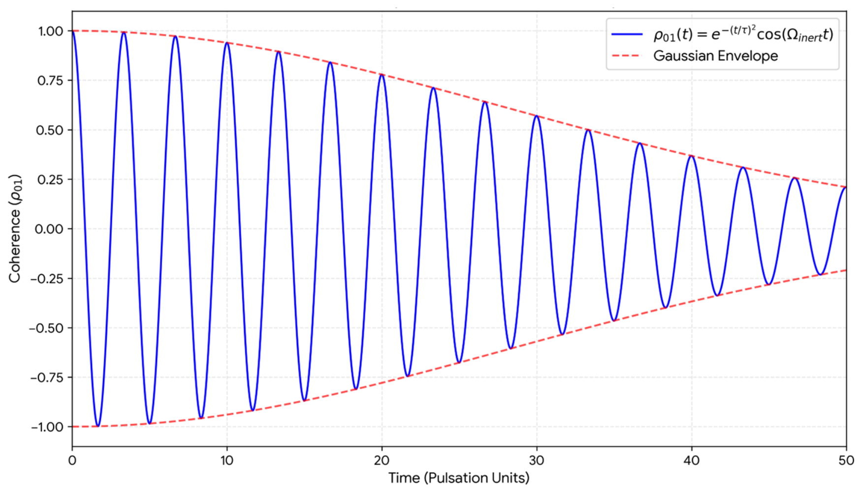
In such an approach, coherence is not lost to a random “environment” (as in standard decoherence theory). Instead, it is periodically exchanged with the inerton field. Then the coherence density can be simulated by the formula

$${\rho }_{01}=e^{-{(t/\tau )}^2}·\cos ({\mathsf{\Omega }}_{\mathrm{inert}} t)$$

(29)

The cosine term represents the periodicity. Because the particle is constantly pulsating into an inerton cloud and back, the coherence “shivers”. When the particle is in its inerton cloud state, its information is spread across the tessellattice; when it returns to the particle state, the coherence “refocuses”. The Gaussian term represents the inerton field effect as a kind of diffusion. While the pulsation is periodic, some energy/information leaks into the surrounding tessellattice cells over time. This is the “damping” effect caused by the inerton field acting as a submicroscopic medium. The graph corresponding the law (29) is shown in Figure 7.

This periodic recovery of coherence reflects the deterministic exchange of information between the particle and the local space tessellattice cells. In fact, let us check the decay validity. At 50 units (1 ms), the coherence has only dropped to about $0.2$1, which visually appears as a very gradual, slow “ringing down” rather than a sudden drop. These values are physically realistic for quantum systems where the environment allows for extended quantum memory.

Why is this configuration (Figure 7) unique? Because standard quantum mechanics uses a simple exponential decay ($e^{-t/T_2}$) for decoherence. The configuration based on the inerton cloud stability is different because it predicts coherence revivals; i.e., the cosine peaks mean that for a split second during each pulsation, the qubit is more coherent than a standard model would predict. The configuration is deterministic: the “noise” causing the decay is actually a structured field (the inertons), not just random thermal chaos.

This law (29) provides a link between the pure wave penetration and the practical problem of quantum computing (qubit stability). It shows that the “shivering” graphed in the noise spectrum of Figure 7 is the same mechanism that limits the life of a qubit.

The slow decay seen at 50 units indicates that the inerton-induced dephasing is significantly weaker than the qubit’s operational speed, suggesting high quantum gate fidelity.

Finally, let us examine how the proposed model reproduces the experimentally observed decoherence spectra $S\left(\omega \right)$, including $1/f$-noise, thermal noise, and fractional photon noise.

The tessellattice can be integrated into the standard theory of open quantum systems, which requires superimposing the massotension field fluctuations directly onto the standard system-bath paradigm. We can start with the effective interaction Hamiltonian governing the coupling of the qubit to the tessellattice. The qubit is modelled as a two-level system under the influence of local fluctuations of the massotension metric $∆\varsigma \left(t\right)$:

$$H_{\mathrm{int}}=g_{\mathrm{eff}}{ \sigma }_{z }\otimes ∆\varsigma \left(t\right)$$

(30)

where ${ \sigma }_{z }$ is the qubit degree of freedom, $g_{\mathrm{eff}}$ is the coupling constant proportional to the particle’s rest mass, and $∆\varsigma \left(t\right)$ is the stochastic field operator representing the collective tension fluctuations of the tessellattice cells. This model interaction proposes a deeper, submicroscopic origin for these environments.

The stochastic evolution of $∆\varsigma \left(t\right)$ possesses a correlation function whose spectral density $S\left(\omega \right)={\int }_{-\infty }^{\infty }\langle ∆\varsigma \left(t\right)∆\varsigma \left(0\right)\rangle e^{i\omega t}dt$ mirrors conventional noise profiles under specific boundary conditions: (i) at low frequencies, a distribution of defects in the tessellattice produces the classic $1/f$ power spectrum; (ii) at thermal equilibrium, the fluctuations obey the fluctuation–dissipation theorem, matching standard thermal noise.

The massotension framework maps directly into these established $S\left(\omega \right)$ spectra, making the model testable via standard dephasing ($T_2$) and relaxation ($T_1$) measurements.

In a $1/f^{\alpha }$ noise spectrum, $\alpha \approx 1$ can be calculated using the standard model network [52,53,54]. These entities are regions of the tessellattice undergoing massotension fluctuations. Let a defect in the tessellattice fluctuate between two massotension states with a characteristic relaxation time $\tau$. Mathematically, this is modelled as a Random Telegraph Signal (RTS) [52,53,54]. The autocorrelation function of this single fluctuating region exhibits an exponential decay:

$$\langle ∆{\varsigma }_j\left(t\right)∆{\varsigma }_j\left(0\right)\rangle ={\sigma }_j^2{e}^{-t/\tau }$$

(31)

where ${\sigma }_i^2$ is the fluctuation variance of that specific region.

By the Wiener–Khinchin theorem, the noise power spectral density $S_j\left(\omega \right)$ of this region is the Fourier transform of its autocorrelation function:

$$S_j\left(\omega \right)={\int }_{-\infty }^{\infty }{\sigma }_j^2{e}^{-\left|t\right|/\tau } e^{-i\omega t}dt={\displaystyle \frac{2{\sigma }_j^2\tau }{1+{\omega }^{2 }{\tau }^2}}.$$

(32)

This yields a standard Lorentzian spectrum [52,53,54]. At low frequencies ($\omega \ll 1/\tau )$, the spectrum is flat, while at high frequencies ($\omega \gg 1/\tau )$, it drops off as $1/{\omega }^2$. To find the total spectral density $S\left(\omega \right)$ of the entire tessellattice, we integrate the single Lorentzian spectrum over a broad $1/\tau$ distribution of relaxation times, governed by then distribution function $P\left(\tau \right)\propto 1/\tau$:

$$S\left(\omega \right)={\int }_{{\mathsf{\tau }}_{\min }}^{{\mathsf{\tau }}_{\max }}{S}_j\left(\omega \right)P\left(\tau \right)d\tau \propto {\int }_{{\mathsf{\tau }}_{\min }}^{{\mathsf{\tau }}_{\max }}{\displaystyle \frac{2{\sigma }_j^2\tau }{1+{\omega }^{2 }{\tau }^2}}{\displaystyle \frac{1}{\tau }}d\tau ={\int }_{{\mathsf{\tau }}_{\min }}^{{\mathsf{\tau }}_{\max }}{\displaystyle \frac{2{\sigma }_j^2}{1+{\omega }^{2 }{\tau }^2}}d\tau ={\displaystyle \frac{2{\sigma }^2}{\omega }}[\arctan \left(\omega {\mathsf{\tau }}_{\max }\right)-\arctan \left(\omega {\mathsf{\tau }}_{\min }\right)].$$

(33)

For a wide range of frequencies nested comfortably between the boundaries of the tessellattice dynamics ($1/{\tau }_{\max } \ll \omega \ll 1/{\tau }_{\min }$), we apply the approximations $\arctan \left(\omega {\mathsf{\tau }}_{\max }\right)\approx \pi /2$ and $\arctan \left(\omega {\mathsf{\tau }}_{\min }\right)\approx 0$. Substituting these back into the expression (33) yields the textbook relationship

$$S\left(\omega \right)\propto {\displaystyle \frac{\pi {\sigma }^2}{\omega }}, ⟹ S\left(\omega \right)\propto {\omega }^{-1}.$$

(34)

If the distribution of activation energies $P\left(E\right)$, which influences the relaxation time $\tau$, deviates slightly from being perfectly uniform, the exponent shifts from exactly 1, resulting in the more general form

$$S\left(\omega \right)\propto {\omega }^{-\alpha }, \alpha \approx 1.$$

(35)

When a qubit is exposed to the total noise spectrum $S\left(\omega \right)$ derived by the ensemble of tessellattice cells, its phase coherence decays over time. The pure dephasing rate (${\Gamma }_{\varphi }=1/T_{\varphi }$), which typically dominates the total dephasing rate ($1/T_2)$, is calculated by integrating the noise spectrum multiplied by the qubit’s operational filter function $F\left(\omega \right)$,

$${\displaystyle \frac{1}{T_2}}\approx {\displaystyle \frac{1}{2T_1}}+{\displaystyle \frac{1}{2\pi }}{\int }_{{\omega }_{\min }}^{\infty }S\left(\omega \right)F\left(\omega \right)d\omega .$$

(36)

For a standard free-induction decay measurement (a Ramsey experiment), the filter function is $F\left(\omega \right)={\sin }^2(\omega t/2)/{(\omega /2)}^2$ [55]. Substituting the derived $1/f$ noise spectrum $S\left(\omega \right)=A/\omega$ into Equation (36), we obtain

$${\displaystyle \frac{1}{T_2}}\propto {\int }_{{\omega }_{\min }}^{{\omega }_{\max }}{\displaystyle \frac{A}{\omega }}·{\displaystyle \frac{ {\sin }^2(\omega t/2)}{{(\omega /2)}^2}}d\omega .$$

(37)

Here, the integral diverges logarithmically at the low-frequency limit. Hence, the low-frequency cutoff can be determined by the total experimental observation time ($t_{\exp }$), meaning ${\omega }_{\min }\cong 1/t_{\exp }$. Evaluating this integral leads directly to the standard condensed-matter relation for $1/f$ dephasing:

$${\displaystyle \frac{1}{T_2}}\propto A \ln \left({\displaystyle \frac{{\omega }_{\max }}{{\omega }_{\min }}}\right).$$

(38)

The temporal dynamics of this system span three distinct scales: $\tau$ (the environmental micro-time) represents the local fluctuation lifetime of a tessellattice region switching between massotension states; $S\left(\omega \right)$ (the spectral bridge) is the total frequency-domain noise power produced by the ensemble integration of individual $\tau$ modes; and $T_2$ (the macroscopic qubit coherence time) is the measurable lifetime of the qubit’s quantum superposition, which scales inversely with the amplitude $A$ of the integrated $1/f$ noise spectrum.

In quantum information frameworks, the standard method for calculating $1/f$-driven $T_2$ times relies precisely on this classical scheme [52,53,54]. Here, the broad distribution of two-level fluctuators maps onto uniform matrix boundaries accompanied by spatial oscillations from individual tessellattice cells, while stochastic phase jumps (${\sigma }_z$) directly emerge from underlying massotension fluctuations.

8. Discussion

The massotension field, whose carriers are inertons, is as fundamental in the universe as the electromagnetic field, whose carriers are photons. Within a real-space continuum constructed as a tessellattice of primary topological balls, these two fields represent the only fundamental manifestations of structural dynamics: the massotension field governs volumetric transformations, whereas the electromagnetic field governs surface area deformations of individual tessellattice cells.

A defining characteristic of any dynamic system is the process of breathing. For quantum systems, this manifests as a submicroscopic, breathing-like oscillatory mass–energy exchange mediated by photons and inertons. This periodic interaction provides intrinsic stability to quantum entities. Consequently, decoherence should not be viewed merely as an abstract fading away of a quantum state, but rather as a dynamical manifestation of this fundamental environmental breathing process.

This submicroscopic perspective carries profound implications for the four strategic pillars of modern quantum technologies: (i) quantum computing and simulation, (ii) quantum communication and cryptography, (iii) quantum sensing and metrology, and (iv) quantum materials and devices. Currently, massive academic and financial investments are directed toward developing physical qubit frameworks, such as superconducting circuits, trapped ions, neutral atoms, spin quantum dots, and photonic systems.

However, standard development frameworks treat these qubits in isolation from their continuous interaction with the primary subquantum environment. Current models rely strictly on the abstract mathematical formalism of quantum mechanics, which quantifies natural oscillatory movements through a purely statistical lens of probability and stochastic processes.

When scaled to complex structures involving hundreds of qubits and thousands of sequential gates, this purely abstract approach becomes fundamentally unreliable. It lacks a mechanistic understanding of the submicroscopic internal processes governing qubit operations and inter-qubit cross-talk. Consequently, the rapid accumulation of logical errors—which engineers attempt to mitigate by exponentially scaling physical qubit overhead for error correction—stems largely from an incomplete understanding of how quantum systems behave within real, physical space.

In conventional computing, information is binary and bound to discrete states ($0$ or $1$). Quantum computing leverages the wave-like nature of matter to operate via state superpositions, where a qubit is mathematically defined as a state vector on the Bloch sphere,

$$\left|\psi ⟩=\alpha \right|0⟩+\beta |1⟩.$$

Here, α and β are complex amplitudes satisfying the Born rule, where the probability of a given measurement outcome scales as ${\left|\alpha \right|}^2$. Entanglement extends this framework via tensor products to scale the underlying vector space exponentially ($2^n$), while unitary matrices model gate operations that exploit constructive and destructive phase interference to filter out erroneous computational paths.

While this algebraic framework is mathematically elegant, it functions as a theoretical abstraction. In physical nanochips and sub-nanochips, the ideal purity of these unitary matrices is disrupted by extrinsic noise fluctuations, leading to state leakage and stochastic gate failures. Researchers are currently constrained by a “black box” paradigm born from the conventional view of the quantum vacuum as a sterile, zero-point void. Trapped in this view, current engineering approaches attempt to suppress decoherence solely through massive cryogenic, sub-Kelvin infrastructure, rather than exploiting materials optimised for inerton resonance and field suppression.

The shift toward a classical wave description within a discrete tessellattice space substrate provides actionable avenues for quantum engineering that bypass these thermal constraints. By transitioning from a probabilistic framework to a deterministic, material-based approach, the submicroscopic physics of inertons can be directly exploited to engineer noise-resilient hardware through three primary applications:

• Substrate Metamaterial Engineering: Instead of fighting vacuum fluctuations with extreme dilution refrigerators, engineers can design quantum chip substrates using specialised crystal geometries. By tailoring the mechanical and lattice properties of the substrate, it becomes possible to create “inerton bandgaps” that actively deflect isolating the qubit from its ambient environment.
• Inerton-Targeted Dynamical Decoupling: Current quantum error mitigation uses electromagnetic pulses to refocus qubits (dynamical decoupling). Integrating our model allows engineers to calculate the exact periodicities of the submicroscopic “environmental breathing.” Control pulses can then be tuned to the precise frequencies of local inerton field oscillations, neutralising phase errors before they manifest mathematically on the Bloch sphere.
• Mass-Isolated Configurations: Because inertons represent mass–energy exchanges within the tessellattice, the physical mass and geometric volume of the qubit junctions themselves dictate their coupling strength to the vacuum noise. Designing qubits with optimised sub-nanometre mass profiles can minimise their cross-section to local massotension field gradients, inherently lowering baseline decoherence rates at ambient temperatures.

The existence of a fundamental inerton field implies that the current path toward scaling quantum computers will inevitably hit an asymptotic scaling limit. High error rates will persist as long as the physical mechanism driving these perturbations—inerton field fluctuations—is ignored.

This challenge can be addressed within an expanded knowledge base. By integrating inerton-gradient metrological monitors (functioning as quantum “weather stations”) alongside localised, coherent inerton emission fields, it becomes possible to map the intensity and frequency of ambient inerton oscillations. This approach paves the way for advanced chip architectures designed to navigate or “float” through the background field without decohering, potentially eliminating the requirement for extreme cryogenic cooling.

Furthermore, because inertons act as the underlying carriers of quantum-mechanical interactions, they open new frontiers in communication. Free inerton propagation velocities are estimated to exceed the speed of light by one to two orders of magnitude, offering an alternative pathway beyond standard quantum key distribution (QKD). In metrology, measuring the gradient of the local inerton–gravitational field offers a paradigm shift for autonomous, high-precision inertial navigation without relying on external satellite-based GPS infrastructure.

9. Conclusions

To advance the empirical validation of inerton physics within the quantum domain, future research must prioritise the following key areas:

• Conducting systematic investigations into how specific condensed-matter systems (such as customised crystal lattices, liquids, or low-temperature plasmas) dynamically respond to inerton field coupling {sensor material optimisation}.
• Developing filtering methodologies to cleanly isolate and distinguish submicroscopic inerton signals from standard electromagnetic and thermal noise backgrounds {signal-to-noise verification}.
• Achieving experimental quantification demonstrating that a controlled shift in the local massotension field gradient induces a predictable, mathematically verifiable change in the error rates of adjacent qubits {empirical mathematical correlation}.
• Establishing rigorous physical criteria for inerton field coherence and decoherence to design active noise-suppression mechanisms for physical qubits {coherence and suppression criteria}.