Abstract
We review recent results on quantum one-way functions, including quantum fingerprinting or quantum hashing (we use these two terms as synonyms even though they have very small difference). This includes the analysis of their properties, different modifications, circuit implementation on an IBM Q platform, as well as on an experimental quantum setup. We discuss computational aspects of quantum hashing, its cryptographic properties and possible usage in communication protocols and algorithms.
1. Introduction
Quantum computing [1,2,3] has been one of the hottest topics in computer science over the last few decades. There are many problems in which quantum algorithms outperform the best known classical ones [4]. One of the useful techniques for constructing algorithms in different computational models is quantum hashing or quantum fingerprinting. In classical computation, hash functions are widely used in algorithms and data structure design [5,6]. As an example, we can consider the Rabin–Karp algorithm for the string matching problem [7], the hash table data structure [8,9,10], and the comparison of objects in standard libraries of programming languages [11]. One of the popular applications is cryptography [6,12]. Cryptography applications involve the use of one-way functions as hash functions because of their cryptographic properties.
In quantum computing, hash functions also have many applications in algorithm design, including cryptography [13,14,15,16,17,18,19], where one-way property is crucial. Quantum one-way functions can be categorized into four types. The categorization is based on their input–output formats:
- Classical–classical: These functions retain a classical nature but satisfy the properties of quantum one-wayness. Their relevance is demonstrated in statistical zero-knowledge protocols and quantum oracle indistinguishability tasks [20,21].
- Classical–quantum: This type is extensively explored in the context of quantum hash functions [22,23,24,25]. Applications include signing classical data [26] and quantum digital signature schemes [27].
- Quantum–classical: These functions enable the authentication of quantum states via classical strings. The work of Behera et al. illustrates their utility in enhanced quantum money schemes [28].
- Quantum–quantum: These directly transform quantum states into other quantum states. The first implementation, proposed by Shang et al. [29], combines “quantum–classical” and “classical–quantum” quantum one-way functions. This approach is successfully applied in quantum identity authentication protocols, where one quantum state verifies the authenticity of another.
In this paper, we focus on the Classical–quantum type of one-way functions as quantum hash functions.
Another name for the same technique is “fingerprinting”. The probabilistic (randomized) technique was developed by Frievalds [30,31]. The main idea of the technique is to randomly choose one of specially constructed hash functions from a given set and to use it for comparing objects for equality. Here, the value of a hash function is called a “fingerprint” of an object.
A thoughtful reader can see a difference between the “hash function technique” and the “fingerprinting technique”. At the same time, the nature and key idea of the techniques are the same. That is why we use these terms as synonyms in this paper.
The quantum version of the fingerprinting technique was developed by Ambainis and Frievalds [32] for automata and later improved by Ambainis and Nahimovs in [33,34]. Later, Buhrman et al. in [22] provided an explicit definition of the quantum fingerprinting algorithm to construct an efficient quantum communication protocol for equality testing. The technique was applied to branching programs by Ablayev, Vasiliev, and Gainutdinova [35,36,37], this computational model can be considered as a non-uniform automata. They show examples of Boolean functions that can be computed by a quantum branching program with exponentially smaller complexity (width or states in terms of automata) than the deterministic ones. Based on this research, they developed the concept of cryptographic quantum hashing [23,24]. Later, they generalized the technique and suggested a family of quantum hashes that allow us to see a trade-off between one-way resistance and collision resistance of the hash function [25,38,39]. Different versions of hash functions were applied that are hash functions in the case of finite abelian groups [40] and arbitrary groups [41], as well as functions based on graphs [26,42]. An alternative approach for cryptographic ideas was presented in [43]. The connection of the approach with the quantum Fourier transform is presented in [44,45]. We define the concept of quantum hashing and discuss its properties in Section 3.
Similarly to classical hash functions, quantum hash functions have parameters that allow them to satisfy required properties and to be useful for comparing objects. We discuss procedures for computing parameters of the quantum hash functions in Section 5.
Turaykhanov, Akat’ev, and coauthors implemented a technique in a photon-based real quantum device [46]. The technique was extended to qudits, and this extension was used in the experimental implementation [47]. Alternative photon-based real quantum device implementation was developed by Plachta, Hiekkamäki, Yakaryılmaz, and Fickler [48] and Zhao, Li, Li, Zheng, and He [49]. The experiments and the qudit version of the method are presented in Section 4.
In the discussed experiments, the algorithm was embedded in this device. When we discuss the implementation of the algorithm for “universal” quantum devices such as IBMQ quantum computers or similar, we should represent the algorithm as a quantum circuit. It is important to minimize the number of quantum gates in the circuit with respect to the architecture restrictions of a quantum device. Optimization for quantum computer emulators was explored in [50]. A shallow circuit for the algorithm was suggested in [51,52]. Its implementation on a real quantum computer’s noisy simulators was discussed in [45,53,54,55]. We present the results in Section 6.
This approach has been widely used in various areas such as stream processing algorithms [56], query model algorithms [57,58], online algorithms [59,60], quantum online algorithms with restricted size of memory [61,62], branching programs [63,64], development of quantum devices [65], automata [66,67,68], and others. Several applications are discussed in Section 7.
2. Preliminaries and Definitions
Here, we present short notes on quantum computation. The reader can find more information about quantum circuits in [1,3].
The notion of a quantum bit (qubit) is the basis of quantum computations. The qubit is the quantum version of the classical binary bit physically realized with a two-state device. Formally, the qubit’s state is the column vector of two-dimensional Hilbert space , that is, Here, the pair of vectors and is an orthonormal basis of , where such that . The numbers are called amplitudes. Consider a qubit in a state such that . Then, we can represent the amplitudes as where , .
A quantum state of a quantum n-qubit register is a complex-valued unit vector in -dimensional Hilbert space that is described as a linear combination of basis vectors: , :
Quantum mechanics postulates that transformations of quantum states (of the quantum n-qubit register) are mathematically determined by unitary operators: where U is a unitary matrix for transforming a vector that represents a state of a quantum n-qubit register.
There is only one way to extract information from the state of a quantum n-register to a “macro world”. It is a measurement of the state of the quantum register. If we measure the quantum state , then we obtain one of the basis states, , with probability .
2.1. Quantum Computational Models
In this paper, we consider different computational models.
2.1.1. Quantum Circuits
One of the most common is the quantum circuit that consists of qubits and gates (unitary transformations). Graphically, on a circuit, qubits are presented as lines.
As basic gates, we consider the following ones:
Additionally, we consider five nonbasic gates:
The two-qubit gates (for example, the CNOT gate) is the most “expensive” for physical implementation. By “expensive”, we mean that both computational error and the difficulty of implementation on a real device are high. So, we consider the number of CNOT gates as a main complexity measure for a circuit. We call it CNOT cost.
At the same time, one two-qubit gate (CNOT gate as an example) and one-qubit gate are the basis for quantum circuits [69].
2.1.2. Quantum Query Model
Another popular model is the quantum query model. Let be an M variable function. We wish to compute on an input . We are given an oracle access to the input x, i.e., it is realized by a specific unitary transformation usually defined as , where the register indicates the index of the variable we are querying, is the output register, and is some auxiliary work space. An algorithm in the query model consists of alternating applications of arbitrary unitary transformations independent of the input and the unitary query, and a measurement in the end. The smallest number of queries for an algorithm that outputs with probability on all x is called the quantum query complexity of the function f.
The model can be considered as a circuit with alternating unitary transformations of two types. The first one is a regular unitary transformation, the second one is a transformation that is controlled by input variables.
Search problem
Suppose that we have a set of objects named , of which some are targets. Suppose that is an oracle that identifies the targets. The goal of a search problem is to find a target by making queries to the oracle .
In search problems, one will try to minimize the number of queries to the oracle. In the classical setting, one needs queries to solve such a problem. Grover, on the other hand, constructed a quantum algorithm that solves the search problem with only queries [70], provided that there is a unique target. When the number of targets is unknown, Brassard et al. designed a modified Grover algorithm that solves the search problem with queries [71], where is the number of targets, which is of the same order as the query complexity of the Grover search.
2.1.3. Branching Programs
A quantum branching program (QBPs) is a known model of computations, a generalization of the classical branching program (BP) model of computations. We refer to [36,64] for more information on QBPs. Quantum branching programs and the quantum query model are closely related. They can be considered as a specific variant of each other depending on the point of view. For example, in the content of this work, QBPs can be considered as a special variant of the quantum query model, which can test only one input variable on a level of computation. Here, we define a QBP as found in [3,72]. Another point of view of the model is the data stream processing algorithms.
3. Quantum Hashing Technique
In this section, we present recent results on quantum hashing developed in our research group.
3.1. One-Way -Resistance
We present the following definition of a quantum -resistant one-way function. Let the “information extracting” mechanism M be a function . Informally speaking, the mechanism M makes some measurement to state and decodes the result of the measurement to .
Definition 1.
Let X be a random variable distributed over like . Let be a quantum function. Let Y be any random variable over obtained by some mechanism M, causing a measurement to encode ψ of X and decoding the measurement result into . Let . We call a quantum function ψ a one-way δ-resistant function if the following apply:
- It is easy to compute, i.e., a quantum state for a particular can be determined using a polynomial-time algorithm;
- For any mechanism M, the probability that M successfully decodes Y is bounded by δ:
For cryptographic purposes, it is natural to expect (and this is applied in the rest of the paper) that the random variable X is uniformly distributed.
A quantum state of qubits can “carry” an infinite amount of information. On the other hand, the fundamental result of quantum informatics known as Holevo’s Theorem [73] states that a quantum measurement can only give bits of information about the state. Here, we use the result of [74] motivated by Holevo’s Theorem.
Property 1.
Let X be a random variable uniformly distributed over . Let be a quantum function. Let Y be a random variable over obtained by some mechanism M making some measurement of the encoding ψ of X and decoding the measurement result to . Then, the probability of correct decoding is given by
3.2. Collision -Resistance
The following definition was presented in [75].
Definition 2.
Let . We call a quantum function a collision ϵ-resistant function if for any pair of different inputs,
Testing equality.
The crucial procedure for quantum hashing is an equality test for and that can be used to compare encoded classical messages v and w; see, for example, [27]. This procedure can be a well-known SWAP-test [22] or one that is adapted for specific hashing functions, like the REVERSE-test; see [23].
3.3. Balanced Quantum -Resistance
The above two definitions and considerations lead to the following formalization of the quantum cryptographic (one-way and collision resistant) function.
Definition 3.
Let and . Let and . We call a function a quantum -resistant -hash function (or just quantum -hash function) iff ψ is a one-way δ-resistant and a collision ϵ-resistant function.
Let for some finite alphabet Σ, with an integer . In which case, we call the function (m,ϵ,s)-quantum hash function if ψ is ϵ-resistant.
We present below the following two examples to demonstrate how one-way -resistance and collision -resistance are correlated. The first example was presented in [32] in terms of quantum automata.
Example 1.
Let us encode numbers v from by a single qubit as follows:
Extracting information from by measuring with respect to the basis gives the following result. The function is one-way -resistant (see Property 1) and collision -resistant. Thus, the function has a good one-way property, but has a bad collision resistance property for large k.
Example 2.
Let . We encode v by k qubits: .
Extracting information from by measuring with respect to the basis ,…, gives the following result. The function is one-way 1-resistant and collision 0-resistant. So, in contrast to Example 1, the encoding from Example 2 is collision-free, that is, for different words v and w, the quantum states and are orthogonal and therefore reliably distinguished; but we lose the one-way property, i.e., is easily invertible.
The following result [75] shows that a quantum collision -resistant function needs at least qubits.
Property 2.
Let and . Let be a collision ϵ-resistant quantum hash function. Then,
Proof.
See [75] for the proof. □
Properties 1 and 2 provide a basis for building a “balanced” one-way -resistance and collision -resistance properties. That is, roughly speaking, if we need to hash elements w from the domain with and if one can build for an a collision -resistant hash function with qubits, then the function f is one-way -resistant with . Such a function is balanced with respect to Property 2.
To summarize the above considerations, we can state the following. A quantum -hash function is a function that satisfies all of the properties that a “classical” hash function should satisfy. Pre-image resistance follows from Property 1. The second pre-image and collision resistance follow, because all inputs are mapped to states that are nearly orthogonal. Therefore, we see that quantum hash functions can satisfy the three properties of a classical cryptographic hash function.
3.4. Quantum -Hash Function Construction via Small-Biased Sets
This section is based on [40]. We present here a brief background on -biased sets as defined in [76] and discuss their connection to quantum hashing. Note that -biased sets are generally defined for arbitrary finite groups, but here we restrict ourselves to .
For an , a character of is a homomorphism , where is the (multiplicative) group of complex q-th roots of unity. That is, , where is a primitive q-th root of unity. The character is called a trivial character.
Definition 4.
A set is called ϵ-biased if for any nontrivial character ,
These sets are interesting when (as is 0-biased). In their seminal paper, Naor and Naor [77] defined these small-biased sets, gave the first explicit constructions of such sets, and demonstrated the power of small-biased sets for several applications.
Remark 1.
Note that a set S of elements selected uniformly at random from is ϵ-biased with positive probability [78].
Many other constructions of small-biased sets followed over the last few decades.
Vasiliev [40] showed that -biased sets generate (,)-resistant hash functions. We present the result of [40] in the following form.
Property 3.
Let be an ϵ-biased set. Let
be a set of functions determined by S. Then, a quantum function
is a -resistant quantum hash function, where .
Proof.
The one-way -resistance property of follows from Property 1: the probability of correctly decoding an x from a quantum state is bounded by . The efficient computability of such a function follows from the fact that any quantum transformation on s qubits (including the one that creates a quantum hash) can be performed with elementary quantum gates [1]. Whenever , this number of steps is polynomial in (the binary representation of group elements) and .
The collision -resistance property of follows directly from the corresponding property of [40]. Note that
The remainder of this proof coincides with the proof of the paper [40]. □
Remark 2.
It is natural to call the set of functions a uniform -biased quantum hash generator in the context of the definition of a quantum hash generator from [24] and the above considerations.
As a corollary of Property 3 and the above considerations, we can state the following.
Property 4.
For a small sized ϵ-biased set with , for , a quantum hash generator generates the balanced -resistant quantum hash function given by
3.5. Quantum Hashing for Finite Abelian Groups
In [40], we proposed the notion of a quantum hash function, which is defined for arbitrary finite abelian groups.
Let G be a finite abelian group with characters , indexed by . Let be an -biased set for some .
Definition 5.
We define a quantum hash function as follows:
We have shown that has all the properties of a cryptographic quantum hash function (i.e., it is quantum one-way and collision-resistant), which are entirely determined by the -biased set .
There are two known special cases of quantum hashing for specific finite abelian groups, which turn out to be the known quantum fingerprinting method. In particular, we are interested in hashing binary strings, and thus, it is natural to consider and (or, more generally, any cyclic group ).
Hashing the elements of the Boolean cube.
For , its characters can be written in the form , and the corresponding quantum hash function is the following:
The resulting hash function is exactly the quantum fingerprinting by Buhrman et al. [22], once we consider an error-correcting code, whose matrix is built from the elements of S. Indeed, as stated in [79] an -balanced error-correcting code can be constructed out of an -biased set. Thus, the inner product in the exponent is equivalent to the corresponding bit of the codeword, and altogether, this gives the quantum fingerprinting function, which stores information in the phase of quantum states [80].
Hashing the elements of the cyclic group
For , its characters can be written as , and the corresponding quantum hash function is given by
The above quantum hash function is essentially equivalent to the one we have defined earlier in [23], which is in turn based on the quantum fingerprinting function from [37].
3.6. Single-Qubit Version of Quantum Hashing
In [46], we constructed an OAM-based version of the quantum hash function, which was defined as follows.
For the classical input , we create its quantum image composed of s single-photon states:
where are numeric parameters of the quantum hash function that provide its collision resistance.
The main idea behind quantum hashing is to provide the minimal fidelity of different quantum hash codes (collision resistance) with the minimal possible number of qubits (that affects the one-way property). As mentioned in [25], there is always a trade-off between these two properties, so balancing them in a quantum hash function is an important task.
The fidelity of and is given by , and for the OAM-based hash function above, it is equal to
Thus, from (18), the set of parameters should give the minimal fidelity of all pairs of unequal and , i.e.,
In [81], we proved the existence of the parameter set described by Formula (19). The proof develops the ideas from [32] and uses a similar notion of the “good” parameters. The following lemma has been proven.
Lemma 1.
There is a set with , which is “good” for all .
In [82], the following connection between the single-qubit version and the “entangled” version was shown. Let be the number of qubits. Let , and consider a special case where elements of are equal to sums of all possible subsets of B, i.e., for ,
Then, the following holds:
Thus, the quantum hash function can be computed by a circuit that has just two layers—the first layer contains Hadamard gates for all qubits, and the second layer contains single-qubit gates equivalent to rotations. To do so, we need to choose the set of parameters that generates the -biased set S according to Equation (20).
3.7. Multiqudit Quantum Hashing
In [47], we defined another version of the quantum hashing technique for a cyclic group, i.e., we considered and . It is based on small-biased sets and high-dimensional states (qudits). But first, we note the following equivalence between -biased sets.
Property 5.
Let and . Then, for any , i.e., the set S is equivalent (in terms of its bias) to .
Proof.
The proof of this statement is based on the following considerations:
therefore,
□
Now, let be the -biased subsets of , and we denote for . By Property 5, without loss of generality, we may consider all to be equal 0. In other words, for all it holds that
Then, for , we define a multiqudit quantum hash function in the following way:
where are the basis states (; d is the dimension of the qudit state space), q is the size of the input state space, is a classical input that is encoded by the relative phase of m qudit states, and are numeric parameters (elements of the -biased sets) of the quantum hash function that provide its collision resistance. The main idea of the collision resistance property is to provide minimum fidelity between different quantum hashes (quantum hash function images) with the minimum possible number of quantum information carriers. Furthermore, reaching a reasonable balance between collision resistance property and one-way property for a quantum hash function is also an important task.
Note that the formula for gives the classical–quantum function that transforms a classical input into the quantum state composed of m qudits (d-dimensional systems). The same state can be constructed with an appropriate number of 2-dimensional systems (qubits); however, this would imply creating entangled states, which are harder to create and maintain.
Theorem 1.
Proof.
According to Definition 3, we need to show two main properties for the function :
- -One-wayness: The dimension of the input space is q, and the quantum state space has dimension . Thus, is -one-way for
- -Collision resistance: The maximal inner product between unequal quantum hashes is bounded byif all are -biased sets.
Thus, corresponds to the balanced -resistant quantum hash function according to [25]. □
Note that the proof above also suggests that comparing hashes of two different values and is equivalent to comparing hashes of and 0.
Remark 3.
Although ε-biased sets give guaranteed collision resistance to our multiqudit quantum hash function, for small sizes of input and output spaces, better bounds on collision resistance can be obtained by numeric optimization (see Table 1 for details).
At the moment, this approach can be used only for relatively small values of and q since it implies an exhaustive search for optimal values of that give minimum to the following function:
Note that the general lower bound suggests that, for an input state space of size q, a collision probability bounded by implies that a target quantum state space should have a size of at least ). On the other hand, there exist -biased sets of size , and thus, our construction gives the output state space of .

Table 1.
The worst-case values of collision probability with parameters from -biased sets and from the numeric optimization, .
Table 1.
The worst-case values of collision probability with parameters from -biased sets and from the numeric optimization, .
| Number of Qudits | -Biased Sets | Exhaustive Search |
|---|---|---|
| 1 | 0.9998 | 0.9998 |
| 2 | 0.9996 | 0.959 |
| 3 | 0.9994 | 0.7519 |
| 4 | 0.9992 | 0.4378 |
| 5 | 0.999 | 0.2031 |
| 6 | 0.9988 | 0.0806 |
| 7 | 0.9986 | 0.0279 |
| 1 | 0.9681 | 0.9681 |
| 2 | 0.9372 | 0.5422 |
| 3 | 0.9073 | 0.1483 |
| 4 | 0.8784 | 0.0368 |
| 5 | 0.8504 | 0.0063 |
| 1 | 0.8329 | 0.8329 |
| 2 | 0.6937 | 0.2174 |
| 3 | 0.5778 | 0.0429 |
| 4 | 0.4813 | 0.0072 |
4. Implementation of the Multiqudit Quantum Hashing on Real Devices
In the previous section, we suggested quantum hash functions as a sequence of independent qubits, where the classical information was encoded in the qubit phase. Now, we propose a quantum hashing protocol, where the information carriers are high-dimensional states with an orbital angular momentum. In this case, the structure of the quantum hash can be represented by Equations (25) and (26).
Here, we propose the implementation of a verification procedure whereby for a given quantum hash and a classical value , it checks whether or not . The ideal quantum experiment that verifies a multiqubit quantum hash can be set as follows:
- We receive a quantum hash of some generally unknown value as a sequence of m single photons in the overall state :where the j-th qudit is expected to be in the state as described by Equation (25).
- Then, we check whether is equal to some predefined or not. To execute this, we perform measurements that project onto and -phase orthogonal states:where , , and are additional phases responsible for the orthogonality of the states. For example, if we use qutrits (3-dimensional states) as information carriers, the set of is equal to {{},{}}.
- The projection measurements of these states may be sequential or parallel. In the latter case, we have to prepare a complex phase mask on part 2 of SLM1, which is an appropriate superposition of detection masks for and states . The complex mask directs the photons into d detection channels corresponding to the states , respectively. The single-photon detector click in or channels corresponds to the outcome or , respectively.
- If , the detector of the output would always click, while the other detectors would never click.
- If , each of the detectors might click, but the probability of the erroneous outcome “” is bounded by the construction of the quantum hash function .
- If none of the detectors clicked, then the qudit is lost, and we either request for it to be sent again or tolerate the higher error probability.
- If all of m measurements end up with the outcome "", then the final result of the experiment is considered to be “”. Otherwise, if at least one qudit leads to , then the overall result is also "".
The error probability comes from the fidelity between two different quantum hashes, which is
The parameter set is chosen in such a way that the pairs of hashes and give the minimal fidelity for . To measure the collision probability, we compare different quantum hashes in the worst-case scenario when quantum hashes for and have the maximum fidelity for a given set .
The protocol starts with a calibration step on which we adjust the coincidence count rate for the “yes” answer (“”). We perform about 200 projection measurements of equal states and calculate the average coincidence count rate between signal and idler photons. The simultaneous clicks in the idler and signal detectors mean that the idler photon has been prepared in the state and has been successfully projected on the state . We pick the average value as the threshold between “yes” and “no”. In this work, we experimentally evaluate the collision probability for a multiqudit quantum hash function with and three groups of parameters: (i) and , (ii) and , and (iii) and , i.e., we perform experiments with varying numbers of qubits, qutrits, and ququarts. We encode the classical message into the phase of states considered in Section 3.7. Since we consider the worst-case situation, without loss of generality, we can focus on the case when . This can be calculated from
for an optimal (quasioptimal) set of parameters , which in turn is precomputed as
Figure 1 shows the comparison of experimental and theoretical error rates for the worst-case scenario depending on different dimensions of quantum states. The experimental results suggest that the proposed technique can be useful even for small sizes of input and output states. Moreover, it can be seen that the number of information carriers decreases with an increase in their quantum state dimension for an optimal relation between the collision probability and the decoding probability (the probability of extracting the classical input x from the quantum hash). For instance, if we limit the collision probability by 0.25 and the decoding probability by 0.15, the optimal number of qudits to “compress” an 8-bit classical information proves to be for , for , and for . Moreover, according to the Holevo theorem [73], no more information can be extracted from a quantum d-level system than from a classical d-level system, which means that we have a bounded probability (below 1) to extract the information about classical input x.
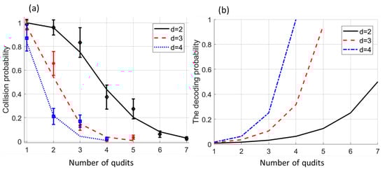
Figure 1.
(a) Comparing experimental and theoretical collision probabilities for the worst-case scenario for different dimensions of quantum states. Vertical lines demonstrate experimental results: the average value of the error in the series of measurements and its standard deviation. (b) The theoretical probability of recovering the original message from its quantum hash.
5. Searching Coefficients
The main properties of the quantum hash function are defined by the set of coefficients S; therefore, it is important to explore methods to find the sets of coefficients that lead to quantum hash functions with a small probability of error. Although there are explicit methods of construction, these are usually slow or their results are worse than those of heuristic methods. This section covers several methods of search, such as brute-force algorithms, random search, genetic algorithms, simulated annealing, and deterministic methods.
Let us define the problem formally. Consider and . First, we choose the size of the parameter set , for example, using Property 2 or Remark 1. Second, we search for the parameter set S such that , where
or is defined in a similar way for the other variants of quantum hash functions. We compare different methods in terms of their running time expressed as a function of q, d, and . Note that we include the time of computing into the whole running time of the algorithm.
In the brute-force method, we systematically check all possible assignments of , . For example, we can start from the assignment , and then move on to the next assignment by increasing the rightmost coefficient that is not equal to along with setting all for . The running time of the brute-force method is .
The random search method takes advantage of Remark 1, and repeatedly chooses a random set S until it satisfies the condition . While this process could be infinite, Remark 1 ensures that for properly chosen d, the expected running time of the algorithm is .
Heuristic algorithms, such as genetic algorithms or simulated annealing, reduce the amount of search space, but may not find the best solution. For example, genetic algorithms use analogies from the evolutionary process. First, they generate the pool of “organisms” (several random sets S); then, they select those that are best suited (i.e., those with smaller ) and “breed” them (i.e., for two sets and , they generate the set for some random ).
Simulated annealing, another heuristic algorithm, likens the search to the heat treatment of steel. It starts with a set , and it sets a parameter T (a “temperature”) to a high value, and then starts to slowly decrease it. At each iteration, the probability of changing a random coefficient to another value depends on temperature and , with higher temperature permitting larger changes. The heuristic algorithms are presented in [38].
Deterministic methods are usually based on derandomization techniques. For example, Khadieva and Ziiatdinov [68] implemented the algorithm described in [83] to compute the parameter set and performed numerical experiments.
6. Circuit Representation of Quantum Hashing and Implementation on Noisy Simulators
6.1. Full Quantum Circuit for Quantum Hashing
The basic implementation part of quantum hashing circuits is a uniformly controlled rotation operator (see Figure 2). We denote the uniformly controlled rotation operator for n control qubits and one target qubit as the operator.
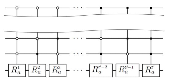
Figure 2.
Quantum circuit for the uniformly controlled rotation operator with d control qubits and rotations by the a axis, that is, z or y.
Here, is the rotation to a angle by the a axis, that is, z or y. It depends on the type of hashing function: y for the amplitude form, and z for the phase form.
Many types of quantum computers (for example, quantum devices based on superconductors) do not allow us to apply two-qubit gates to an arbitrary pair of qubits but have a graph that represents such a restriction. Vertices of the graph correspond to qubits, and two-qubit gates can be applied only to qubits corresponding to vertices connected by an edge. We say that such a graph represents the qubit connection graph for a device.
If the qubit connection graph is complete, i.e., we do not have any restriction on the two-qubit gate application, then the CNOT cost of the uniformly controlled rotation operator is as presented in the following lemma.
Theorem 2.
([84,85]) The CNOT cost of the d-qubit uniformly controlled rotation operator is .
One of the most popular architectures considered by researchers is the linear nearest neighbor (LNN) architecture. The graph for LNN architecture is a chain where the i-th vertex is connected only with vertices and (see Figure 3).

Figure 3.
The linear nearest neighbor (LNN) architecture for 5 qubits.
A circuit for the LNN architecture was presented by Möttönen, Vartiainen, Bergholm, and Salomaa in [84,85] (see Figure 4).
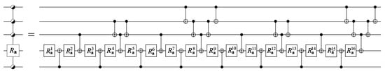
Figure 4.
The quantum circuit for the uniformly controlled rotation gate with 4 control qubits for a linear nearest neighbor (LNN) architecture.
The restriction on architecture slightly affects the CNOT cost, which is discussed in the next theorem.
Theorem 3.
([84,85]) The CNOT cost of the d-qubit uniformly controlled rotation operator for the LNN architecture is .
Zinnatullin, Khadiev, and Khadieva optimized the previous circuit for more complex architectures [50]. A 5-qubit IBM Falcon r4T (Figure 5), 7-qubit IBM Falcon r5.11H (Figure 6), 16-qubit IBM Falcon r4P (Figure 7), and 27-qubit Falcon r5.11(Figure 8) were considered. The CNOT cost for optimized circuits are 20 for a 5-qubit machine, 92 for a 7-qubit machine, 60,716 for a 16-qubit machine, and 100,909,180 for a 27-qubit machine.

Figure 5.
A 5-qubit IBM Falcon r4T architecture.
Figure 6.
A 7-qubit IBM Falcon r5.11H architecture.

Figure 7.
A 16-qubit IBM Falcon r4P architecture.
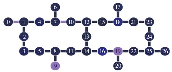
Figure 8.
A 27-qubit IBM Falcon r5.11 architecture.
An application of the presented technique for the representation of the operator as a quantum circuit requires a better precision for the rotation angles than the original one. The original angles require the bit precision (precisely, it is ). At the same time, the presented circuits use angles with bit precision (precisely, it is ). Note that preposition of a rotation angle is a challenging issue for hardware [86]. Khadieva, Salehi, and Yakaryılmaz in [53] proposed a technique that provides a trade-off between CNOT cost and precision for angles. It allows us to obtain any intermediate result between CNOT cost and precision, and CNOT cost and precision.
Each CNOT gate gives us an error probability. Even if the error is very small, the exponential number of CNOT gates dramatically affects the error probability. That is why researchers pay attention to shallow versions of circuits for quantum hashing.
6.2. Shallow Circuit
Kālis (with Ambainis as a supervisor) in his master thesis [51] suggested a shallow circuit for the quantum hashing in amplitude form for 3 qubits. This idea was investigated by Salehi and Yakaryılmaz [87]. Later, the approach was developed in detail and presented in a general way for quantum hashing by Ziatdinov, Khadieva, and Yakaryılmaz [52]. They suggested to use a shallow circuit presented in Figure 9.
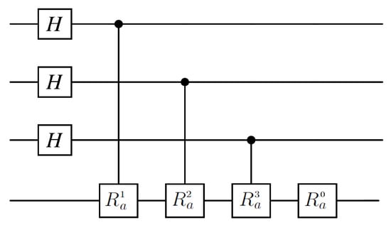
Figure 9.
Shallow quantum circuit for quantum hashing algorithm with 3 control qubits.
If we use the same number of qubits as for the standard circuit with operator, then only independent angles can be chosen. For the angles used in the shallow circuit, we obtain the angles , where is the j-th bit in the binary representation of the integer i. According to [52], it is possible to use generalized arithmetic progressions to find the angles such that the error probability of the quantum hash is comparable to the full quantum circuit, but that requires a large circuit width. The method of finding the angles such that both error probability and circuit width are small remains an open problem.
At the same time, numerical experiments show that we can find a set of angles for such that the error probability of the method is at most . This research is presented in [52].
Ziatdinov, Khadieva, and Khadiev in [54] invoked both circuits on a noisy simulator of an IBM machine for four qubits (three control and one target) for computing mod unary language, where means a string of x symbols 1. By recognizing, we mean returning 1 if the input belongs to , and 0 otherwise. Note that a classical algorithm requires at least bits of memory for recognizing the language [32].
For solving the problem, the authors did not search for angles that minimize the error in an “ideal” (not noisy) device. They used another strategy; they invoked a brute-force algorithm to find the sequence with two properties:
- The probability of accepting member inputs on the noisy simulator should be as high as possible.
- The probability of accepting non-member inputs on the noisy simulator should be as small as possible.
For , the authors minimized a value , , where is the probability of returning 1 for an input . Then, the circuit was invoked for , where . The program was executed 10,000 times and the number of shots that returned the accepting state was the result of computation. We use the notation for this number, where i is the length of the word. The numbers for each length i for are shown in Figure 10. We can say that it is a statistical representation of probability .
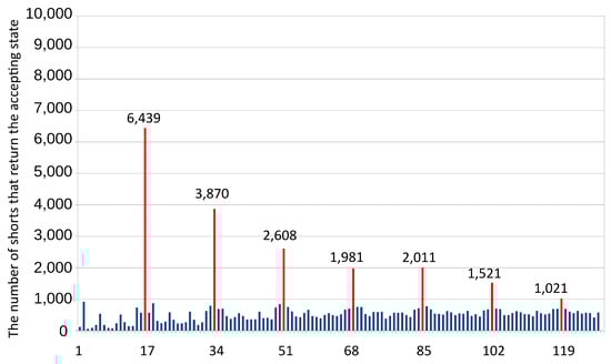
Figure 10.
The number of shots that return the accepting state (Y axis) in the case of a shallow circuit. For different lengths i of the input word, the length of the word (X axis) is .
We can see that each member i of has . At the same time, each non-member i has . So, we can choose a threshold . For any length i, we can say that it is a member iff . Here, we can use the concept of an isolated cutpoint from automata theory [88]. For a cutpoint and constant , we claim that an input is a member of the language if . If an input is a non-member, then .
The authors invoked the same series of experiments for a standard circuit, that is, for . The number of parameters (angles) was too large (it is ) for the brute-force search because the invocation of the circuit on an IBMQ simulator is time-consuming. That is why the coordinate descent method was used for the first six parameters and brute force for the last two parameters. Then, we invoked the circuit for the same inputs for . The result is presented in Figure 11.
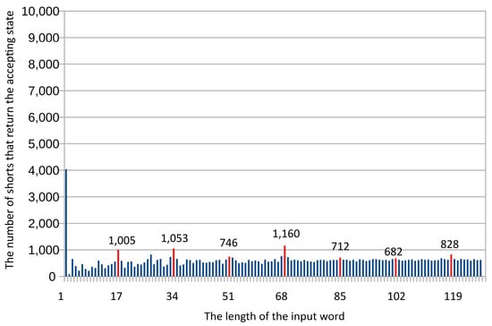
Figure 11.
The number of shots that return the accepting state (Y axis) in the case of a standard circuit. For different lengths i of the input word, the length of the word (X axis) is .
We can see that only a few members like , , , and can be separated from non-members. Other members of cannot be separated from members, for example, , , and . In addition, the result for is larger than for , where . The searching algorithm cannot find a set S that violates this condition. At the same time, we can ignore because it can be checked with additional conditions. Even in this case, the algorithm is only useful for detecting some members with a threshold (or cutpoint) of , but we cannot detect other members.
At the same time, in the case of the shallow circuit, is much higher than for the standard circuit. For instance, for the shallow circuit, which corresponds to provability , while for the standard circuit, the corresponding probability would be much smaller than (approximately ).
These numerical experiments show us that even if for an “ideal” device, the standard circuit with the operator has a smaller error probability than the shallow circuit. In contrast, we have the opposite situation for noisy simulators, where the shallow circuit shows much better results than the standard one.
Vasiliev in [82] considered the phase version of quantum hashing. In this work, rotation was used. The author used the equivalence of and P gates, which are presented in Figure 12.
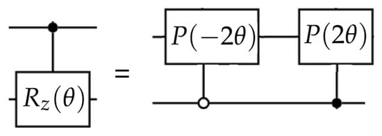
Figure 12.
Equivalence of control and control P gates.
We can use the fact that the target qubit is initially in the state and remove one of two P gates; the remaining P gate can be applied without control. See Figure 13 for the final equivalence of gates.

Figure 13.
Equivalence of control with value for the control qubit and the P gate.
This allows us to convert the shallow circuit for quantum hashing to the circuit without any CNOT gates (see Figure 14).
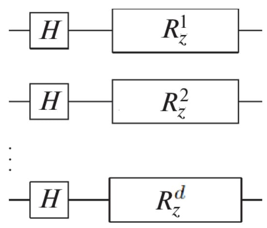
Figure 14.
Shallow circuit for quantum hashing algorithm in phase form in the case of d control qubits.
6.3. Shallow Circuit for LNN Architecture and for Arbitrary Qubit Connection Graphs
Khadieva, Salehi, and Yakaryılmaz [53] suggested a quantum circuit for an LNN architecture (see Figure 15).
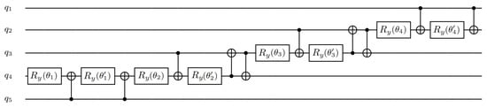
Figure 15.
The shallow quantum circuit for quantum hashing with 4 control qubits for linear nearest neighbor (LNN) architecture.
The main idea is to move the target qubit by the chain using the SWAP gate. The control gate has 2 CNOT cost, the SWAP gate has 3 CNOT cost, but control and SWAP together also have 3 CNOT cost (see Figure 16).
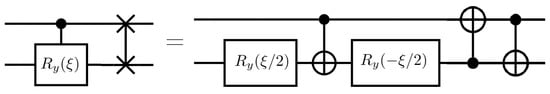
Figure 16.
Representation of sequential control and SWAP gates using only basis gates.
So, this idea allowed the authors to reduce the CNOT cost and obtain the CNOT cost of the circuit that applies quantum hashing ℓ times for d qubits, as presented in the next lemma.
Theorem 4.
([53]) In the case of the LNN architecture, the CNOT cost of a shallow quantum circuit for ℓ applications of quantum hashing with d control qubits is .
Later, Khadieva [45] generalized the technique for more a complex architecture that involves a cycle with tails (like a “sun” and “two joint suns”) represented by a 16-qubit Falcon r4P (see Figure 7) and a 27-qubit Falcon r5.11 IBMQ (see Figure 7) architectures. The CNOT cost of the shallow circuit for the quantum hashing algorithm for these devices is presented in the next lemma.
Theorem 5.
([45]) The CNOT cost of the shallow quantum circuit for ℓ applications of quantum hashing with 15 control qubits is (for ) in the case of the 16-qubit Falcon r4P IBMQ device. The CNOT cost for 26 control qubits is (for ) in the case of the 27-qubit Falcon r4P IBMQ device.
The method was generalized for arbitrary qubit connection graphs by Khadiev, Khadieva, Chen, and Wu in [55]. The authors built the shortest path that visits all vertices at least once. Then, they moved the target qubit by this path using the same technique as for an LNN architecture. They obtained the following complexity for ℓ applications of quantum hashing on d qubits:
Theorem 6.
([55]) Let G be a connected qubit connection graph. The CNOT cost of the circuit for the application of the quantum fingerprinting (quantum hashing) algorithm ℓ times is at most , where k is the length of the shortest path in the graph G that visits all vertices at least once.
Note that the CNOT cost is between and depending on k. If the graph G has a Hamiltonian path, then the cost is minimal.
The shallow quantum circuit for quantum hashing has a structure very similar to the circuit for the quantum Fourier transform (QFT) algorithm [89]. The technique is used in quantum addition [90], quantum phase estimation (QPE) [89,91], quantum amplitude estimation (QAE)[92], the algorithm for solving linear systems of equations [93], Shor’s factoring algorithm [94], 1D wave equation [95], Quantum walks [96,97,98] with applications to quantum backtracking [99,100], and others. The best known representation of the QFT algorithm for LNN architectures is [101], which is an improvement of a series of results [102,103,104,105,106]. At the same time, the presented technique was not applied to general graphs. The authors of [45,55] applied the ideas used for quantum hashing to the QFT algorithm and obtained the CNOT cost for arbitrary qubit connection graphs. Another interesting technique for several specific graphs was discussed in [107].
7. Applications of Quantum Hashing Technique
The quantum hashing technique has been widely used in various areas. Here, we mention only some of the results.
- Stream processing algorithms. Le Gal [56] considered an automata-like model with non-constant size of memory. The technique allowed him to obtain an advantage in memory size for a quantum version of the model. The technique was used for checking the equality of two strings using a logarithmic size of memory.
- Automata. The technique was introduced for an automata model [32] and later improved in [33,34]. The technique allows us to recognize a unary language mod for some prime p. It allows the authors to demonstrate an example of language that can be recognized by a quantum model with an exponentially smaller size of memory compared to the classical (deterministic or probabilistic) counterparts. At the same time, the same technique for the constant number of qubits was used for two-way automata with classical and quantum states [108,109,110,111]. It allows authors to show a language that can be recognizable by the model but cannot be recognizable by the probabilistic two-way automata. Similar results were obtained for one-way models [112,113].Later, the same idea was used for one-way automata and promise problems [66,67,114,115,116,117]. The technique allows showing more languages that can be recognized by the quantum model but cannot be recognized by a classical model [68,118].
- Branching programs. The technique was used for the branching program model by Ablayev, Vasiliev, Gainutdinova, and co-authors [35,36,37]. They showed a family of Boolean functions that can be computed by quantum branching programs with polynomial width (logarithmic size of memory) but cannot be computed by deterministic and probabilistic counterparts. Most of the Boolean functions have an equality of objects (binary strings or other objects) as a base.Later, Khadiev and Khadieva [63] presented an especially constructed Boolean function that allowed them to show a hierarchy of complexity classes for quantum read-k-time branching programs. The upper bound was proven using the quantum fingerprinting technique.Nondeterministic quantum branching programs were investigated by Gainutdinova and co-authors [64,66,119,120,121]. The authors suggested several Boolean functions such that nondeterministic quantum branching programs based on specific versions of quantum hashing can compute them, but classical counterparts cannot.
- Online algorithms with restricted memory size. Quantum algorithms with restricted memory size is a computational model similar to automata but used for online minimization problems [61,62]. Khadiev and Khadieva [59,60] presented a problem that can be solved by quantum online algorithms with a restricted size of memory, but cannot be solved by randomized or deterministic counterparts in the case of logarithmic size of memory. The technique based on one qubit allowed the authors to show a similar result for a constant size of memory [122,123]. The algorithms also used the quantum hashing algorithm for checking the equality of binary strings using a logarithmic size of memory.Similar approaches were used in [124].
- Development of quantum devices.Vasiliev [65] used the technique for developing communication protocols between parts of quantum devices.
- Query model algorithms. Quantum hashing has numerous applications in addressing the string matching problem. The circuit implementation is discussed in [57,58] and the algorithm is presented in detail in the next section.
7.1. Quantum Search in a Dictionary and String Matching Problem
The hashing technique for searches in a database is widely used for compressing data, which allows us to accelerate search procedures. We demonstrate compressing effects and possibilities of the quantum hashing technique based on searches for words in a text.
In this section, we consider the string matching problem. The problem is to search for a word w in a text V. Formally, we should find any index i such that the substring , where is the i-th symbol of V, m is the length of w, and n is the length of V. Here, .
The task of searching for information in a database has been considered in many works and has some specific features. First, the oracle , defined by the task, is used to find the occurrence of the word w in the dictionary V, namely if and only if . Secondly, to speed up the search for a word in a text in the 1970s and 1980s, including hashing-based algorithms were proposed. The Knuth–Morris–Pratt (KMP) algorithm [9,125,126], the Rabin–Karp algorithm [7,8], and the Matiyasevich algorithm [127] can solve the problem in a linear number of comparisons (in linear time), with complexity. Other possible solutions to the problem are Backward Oracle Matching [128], the Wu–Manber algorithm [129], the Boyer–Moore algorithm [130], the algorithms in [131,132] based on suffix arrays [8,131,133,134] and suffix trees [135,136], and others [128,137,138,139].
It is clear that quantum algorithms for this task, based on Grover’s idea [70,92], provide a quadratic saving in the number of calls to the oracle in the quantum query model. Note that to describe Grover’s algorithm, we first need to specify an efficient oracle circuit for for such an algorithm. Several similar studies in recent decades in the field of developing algorithms for the string matching problem have been devoted to the construction of efficient oracles . A number of constructions of such oracles in terms of quantum circuits have been proposed, and the complexity of such circuits have been studied. These include the Practical implementation of a Quantum String Matching Algorithm [140] and the algorithms of Ramesh, Hariharan, and Vinay [141], Montanaro [142], Soni and Rasool [143], and Khadiev and Serov [144]. Note that all of these listed results require qubits.
7.2. Hashing Technique for Quantum Search in the Text
The first idea of using hashing methods for quantum information retrieval in an unordered database was realized in [58]. In this paper, a hybrid classical–quantum (probabilistic-quantum) algorithm is proposed. The key idea of the hybrid classical–quantum algorithm is as follows: (a) choose a universal hash family of hash functions, (b) uniformly randomly choose a hash function , (c) hash the elements of V with the hash function h, and (d) apply the quantum amplification technique to search for the hash image of the word w in the hashed dictionary . It has been proven that using hashing methods can exponentially reduce the number of qubits required. Specifically, qubits are sufficient when using hashing, instead of qubits in algorithms without hashing.
7.3. Search in a Dictionary Based on the Quantum Hashing Technique
The next step in developing a quantum search in a dictionary is based on quantum fingerprinting–hashing and it is presented in [145].
We begin with a discussion of quantum fingerprinting–hashing features that we explored for search in a dictionary. It is important for the above construction that the size of the quantum hash , that is, we have an exponential compression of information.
The quantum hash function defines for the word a unitary transformation:
That is, the operator acts on the space , having as an external control word. It is also convenient to think of this as defining a set of unitary transformations:
In this paper, we assume that the unitary transformation always starts from an initial basis state , that is, we have
For further consideration, we also need the inverse transformation of . Thus, accordingly, for the inverse transformation , the following must be true:
Remark 4.
So, the above definition can be seen as a quantum generalization of the information compression function. On the other hand, we have a quantum hash function ψ and its implementation, the operator . Since the unitary operator is invertible, this means that there are no collisions “in the quantum world”. That is, two different words w and have different hash images and . But we can obtain a collision “in the macro world” (that is, we can decide that the state is generated by the word ) when extracting information about these two different quantum states and . Thus, the probability of such an event (the collision probability) is small when ψ is the collision ϵ-resistant function (see Definition 2).
Now, we present the algorithm based on the technique of ()-quantum hash function works for a quantum solution of the search in a dictionary problem. The sequence of binary words with length m and a binary word w with length m are given. We want to find any index k, which denotes the word number k such that .
Note that the string matching problem can be easily represented as the search in a dictionary problem by taking as a substring of the text string with index i and finishing in .
Thus, the algorithm implements the mapping
The first part of the algorithmconsists of preparing the initial state.
According to this sequence V, using the transformation , which defines the (m,, s)-quantum hash function , a state is prepared:
The second part of the algorithm —amplification—consists of reading a word to be searched for, w, and finding a number k such that . The steps are as follows:
- Conversion hash transformation—first level of amplificationThe operator is applied to the state , where is the inverse transformation controlled by the searched word w. We obtain the statewhere for .
- AmplificationThe amplification of basic states is when “good states” are applied to state . The procedure is described in [92], and is also discussed in the book [146].
- MeasurementThe first qubits of the final state are measured in a computational basis. If the last s qubits are all zero, then the measurement result k of the first qubits is declared as the index of the word in the sequence V, for which .
The algorithm has the following complexity characteristics: searching for a word w of length m in a dictionary V of size n requires qubits. The number of queries (the number of Grover operators applied) is . The key point of the algorithm is the use of the -fingerprinting–hash function to obtain the correct result with high probability.
The steps of the algorithm are as follows: In the first step, the quantum state is quantum-parallel inverted by the mapping defined by w. This step provides the first level of amplitude gain. Then, in the second step, the known sequence of Grover “amplitude amplification operators” is applied. Finally, the resulting quantum state is measured and the algorithm produces the result.
The high probability of a correct result is based on the properties of the quantum hash function—it provides the first level of amplitude amplification before applying the sequence of Grover amplitude amplification operators.
For the formal proof, we refer to [145].
Funding
The research in Section 6 is supported by the Russian Science Foundation Grant 24-21-00406 (https://rscf.ru/en/project/24-21-00406/). M.Z. acknowledges financial support under the National Recovery and Resilience Plan (PNRR), Mission 4, Component 2, Investment 1.4, Call for tender No. 1031 published on 17/06/2022 by the Italian Ministry of University and Research (MUR), funded by the European Union—NextGenerationEU, Project Title "National Centre for HPC, Big Data and Quantum Computing (HPC)"—Code National Center CN00000013—CUP D43C22001240001.
Conflicts of Interest
The authors declare no conflicts of interest.
References
- Nielsen, M.A.; Chuang, I.L. Quantum Computation and Quantum Information, 1st ed.; Cambridge University Press: Cambridge, UK, 2000. [Google Scholar] [CrossRef]
- Ambainis, A. Understanding Quantum Algorithms via Query Complexity. In Proceedings of the International Congress of Mathematicians’2018, Rio de Janeiro, Brazil, 1–9 August 2018; Volume 4, pp. 3283–3304. [Google Scholar]
- Ablayev, F.; Ablayev, M.; Huang, J.Z.; Khadiev, K.; Salikhova, N.; Wu, D. On quantum methods for machine learning problems part I: Quantum tools. Big Data Min. Anal. 2019, 3, 41–55. [Google Scholar] [CrossRef]
- Jordan, S. Quantum Algorithms Zoo. 2025. Available online: http://quantumalgorithmzoo.org/ (accessed on 1 April 2025).
- Konheim, A.G. Hashing in Computer Science: Fifty Years of Slicing and Dicing; John Wiley & Sons: Hoboken, NJ, USA, 2010. [Google Scholar]
- Mehta, D.P.; Sahni, S. Handbook of Data Structures and Applications; Chapman and Hall/CRC: Boca Raton, FL, USA, 2004. [Google Scholar]
- Karp, R.M.; Rabin, M.O. Efficient randomized pattern-matching algorithms. IBM J. Res. Dev. 1987, 31, 249–260. [Google Scholar] [CrossRef]
- Cormen, T.H.; Leiserson, C.E.; Rivest, R.L.; Stein, C. Introduction to Algorithms; McGraw-Hill: New York, NY, USA, 2001. [Google Scholar]
- Knuth, D. Searching and Sorting, the Art of Computer Programming; Reading: Addison-Wesley: Boston, MA, USA, 1973; Volume 3. [Google Scholar]
- Mehlhorn, K.; Sanders, P. Hash tables and associative arrays. In Algorithms and Data Structures: The Basic Toolbox; Springer: Berlin/Heidelberg, Germany, 2008; pp. 81–98. [Google Scholar]
- Oracle Corporation Java® Platform, Standard Edition and Java Development Kit Version 17 API Specification. Class Object. 2025. Available online: https://docs.oracle.com/en/java/javase/17/docs/api/java.base/java/lang/Object.html#hashCode() (accessed on 1 April 2025).
- Menezes, A.J.; Van Oorschot, P.C.; Vanstone, S.A. Handbook of Applied Cryptography; CRC Press: Boca Raton, FL, USA, 1997. [Google Scholar]
- Gisin, N.; Ribordy, G.; Tittel, W.; Zbinden, H. Quantum cryptography. Rev. Mod. Phys. 2002, 74, 145. [Google Scholar] [CrossRef]
- Li, J.; Li, N.; Zhang, Y.; Wen, S.; Du, W.; Chen, W.; Ma, W. A survey on quantum cryptography. Chin. J. Electron. 2018, 27, 223–228. [Google Scholar] [CrossRef]
- Kumar, A.; Garhwal, S. State-of-the-art survey of quantum cryptography. Arch. Comput. Methods Eng. 2021, 28, 3831–3868. [Google Scholar] [CrossRef]
- Moizuddin, M.; Winston, J.; Qayyum, M. A comprehensive survey: Quantum cryptography. In Proceedings of the 2017 2nd International Conference on Anti-Cyber Crimes (ICACC), Abha, Saudi Arabia, 26–27 March 2017; pp. 98–102. [Google Scholar]
- Ablayev, F.; Ablayev, M.; Vasiliev, A.; Ziatdinov, M. Quantum Fingerprinting and Quantum Hashing. Computational and Cryptographical Aspects. Balt. J. Mod. Comput. 2016, 4, 860–875. [Google Scholar] [CrossRef]
- Rozenman, G.G.; Kundu, N.K.; Liu, R.; Zhang, L.; Maslennikov, A.; Reches, Y.; Youm, H.Y. The quantum internet: A synergy of quantum information technologies and 6G networks. IET Quantum Commun. 2023, 4, 147–166. [Google Scholar] [CrossRef]
- Radanliev, P. Artificial intelligence and quantum cryptography. J. Anal. Sci. Technol. 2024, 15, 4. [Google Scholar] [CrossRef]
- Kashefi, E.; Kerenidis, I. Statistical Zero Knowledge and quantum one-way functions. Theor. Comput. Sci. 2007, 378, 101–116. [Google Scholar] [CrossRef]
- Hosoyamada, A.; Yasuda, K. Building quantum-one-way functions from block ciphers: Davies–Meyer and Merkle–Damgard constructions. In Proceedings of the Advances in Cryptology—ASIACRYPT 2018, Brisbane, Australia, 2–6 December 2018; Volume 11272, pp. 275–304. [Google Scholar] [CrossRef]
- Buhrman, H.; Cleve, R.; Watrous, J.; de Wolf, R. Quantum Fingerprinting. Phys. Rev. Lett. 2001, 87, 167902. [Google Scholar] [CrossRef]
- Ablayev, F.; Vasiliev, A. Cryptographic quantum hashing. Laser Phys. Lett. 2014, 11, 025202. [Google Scholar] [CrossRef]
- Ablayev, F.; Ablayev, M. On the concept of cryptographic quantum hashing. Laser Phys. Lett. 2015, 12, 125204. [Google Scholar] [CrossRef]
- Ablayev, F.; Ablayev, M.; Vasiliev, A. On the balanced quantum hashing. J. Phys. Conf. Ser. 2016, 681, 012019. [Google Scholar] [CrossRef]
- Ziatdinov, M. From Graphs to Keyed Quantum Hash Functions. Lobachevskii J. Math. 2016, 37, 704–711. [Google Scholar] [CrossRef]
- Gottesman, D.; Chuang, I. Quantum Digital Signatures. arXiv 2001, arXiv:quant-ph/0105032. [Google Scholar]
- Behera, A.; Paul, G. Quantum to classical one-way function and its applications in quantum money authentication. Quantum Inf. Process. 2018, 17, 1–24. [Google Scholar] [CrossRef]
- Shang, T.; Tang, Y.; Chen, R.; Liu, J. Full quantum one-way function for quantum cryptography. Quantum Eng. 2020, 2, e32. [Google Scholar] [CrossRef]
- Freivalds, R. Fast probabilistic algorithms. In Mathematical Foundations of Computer Science 1979; Becvar, J., Ed.; Springe: Berlin/Heidelberg, Germany, 1979; Volume 74, pp. 57–69. [Google Scholar] [CrossRef]
- Freivalds, R. Probabilistic Two-Way Machines. In Proceedings of the International Symposium on Mathematical Foundations of Computer Science, Pleso, Czechoslovakia, 31 August–4 September 1981; pp. 33–45. [Google Scholar]
- Ambainis, A.; Freivalds, R. 1-way quantum finite automata: Strengths, weaknesses and generalizations. In Proceedings of the 39th IEEE Conference on Foundation of Computer Science, Washington, DC, USA, 8–11 November 1998; pp. 332–342. [Google Scholar] [CrossRef]
- Ambainis, A.; Nahimovs, N. Improved Constructions of Quantum Automata. In Theory of Quantum Computation, Communication, and Cryptography; Kawano, Y., Mosca, M., Eds.; Springer: Berlin/Heidelberg, Germany, 2008; Volume 5106, pp. 47–56. [Google Scholar] [CrossRef]
- Ambainis, A.; Nahimovs, N. Improved constructions of quantum automata. Theor. Comput. Sci. 2009, 410, 1916–1922. [Google Scholar] [CrossRef]
- Gainutdinova, A. On relative complexity of quantum and classical branching programs. Discret. Math. Appl. 2002, 12, 515–526. [Google Scholar] [CrossRef]
- Ablayev, F.; Gainutdinova, A.; Karpinski, M.; Moore, C.; Pollett, C. On the computational power of probabilistic and quantum branching program. Inf. Comput. 2005, 203, 145–162. [Google Scholar] [CrossRef]
- Ablayev, F.; Vasiliev, A. Algorithms for Quantum Branching Programs Based on Fingerprinting. Electron. Proc. Theor. Comput. Sci. 2009, 9, 1–11. [Google Scholar] [CrossRef]
- Vasiliev, A.; Latypov, M.; Ziatdinov, M. Minimizing collisions for quantum hashing. J. Eng. Appl. Sci. 2017, 12, 877–880. [Google Scholar] [CrossRef]
- Ablayev, F.; Ablayev, M.; Vasiliev, A. Quantum hashing and fingerprinting for quantum cryptography and computations. In Proceedings of the International Computer Science Symposium in Russia, Ekaterinburg, Russia, 29 June–3 July 2020; pp. 1–15. [Google Scholar]
- Vasiliev, A. Quantum Hashing for Finite Abelian Groups. Lobachevskii J. Math. 2016, 37, 751–754. [Google Scholar] [CrossRef]
- Ziatdinov, M. Quantum hashing. Group approach. Lobachevskii J. Math. 2016, 37, 222–226. [Google Scholar] [CrossRef]
- Zinnatullin, I. Cryptographic Properties of the Quantum Hashing Based on Expander Graphs. Lobachevskii J. Math. 2023, 44, 776–787. [Google Scholar] [CrossRef]
- Gavinsky, D.; Ito, T. Quantum fingerprints that keep secrets. Quantum Inf. Comput. 2013, 13, 583–606. [Google Scholar] [CrossRef]
- Ablayev, F.; Vasiliev, A. Quantum hashing and Fourier transform. In Journal of Physics: Conference Series; IOP Publishing: Philadelphia, PA, USA, 2020; Volume 1680, p. 012001. [Google Scholar]
- Khadieva, A. Quantum hashing algorithm implementation. arXiv 2024, arXiv:quant-ph/2024. [Google Scholar]
- Turaykhanov, D.A.; Akat’ev, D.O.; Vasiliev, A.V.; Ablayev, F.M.; Kalachev, A.A. Quantum hashing via single-photon states with orbital angular momentum. Phys. Rev. A 2021, 104, 052606. [Google Scholar] [CrossRef]
- Akat’ev, D.; Vasiliev, A.; Shafeev, N.; Ablayev, F.; Kalachev, A. Multiqudit quantum hashing and its implementation based on orbital angular momentum encoding. Laser Phys. Lett. 2022, 19, 125205. [Google Scholar] [CrossRef]
- Plachta, S.Z.; Hiekkamäki, M.; Yakaryılmaz, A.; Fickler, R. Quantum advantage using high-dimensional twisted photons as quantum finite automata. Quantum 2022, 6, 752. [Google Scholar] [CrossRef]
- Zhao, Y.Y.; Li, K.; Li, C.; Zheng, S.; He, Z. Experimental Demonstration Advantage of Photonic Finite Automata. In Proceedings of the 2023 Asia Communications and Photonics Conference/2023 International Photonics and Optoelectronics Meetings (ACP/POEM), Wuhan, China, 4–7 November 2023; pp. 01–03. [Google Scholar]
- Zinnatullin, I.; Khadiev, K.; Khadieva, A. Efficient Implementation of Amplitude Form of Quantum Hashing Using State-of-the-Art Quantum Processors. Russ. Microelectron. 2023, 52, S390–S394. [Google Scholar] [CrossRef]
- Kālis, M. Kvantu Algoritmu Realizācija Fiziskā Kvantu Datorā. Master’s Thesis, University of Latvia, Riga, Latvia, 2018. [Google Scholar]
- Ziiatdinov, M.; Khadieva, A.; Yakaryılmaz, A. GAPs for Shallow Implementation of Quantum Finite Automata. In Proceedings of the 16th International Conference on Automata and Formal Languages (AFL 2023), Eger, Hungary, 5–7 September 2023; Zsolt Gazdag, S.I., Kovasznai, G., Eds.; Open Publishing Association: Waterloo, Australia, 2023; Volume 386, pp. 269–280. [Google Scholar] [CrossRef]
- Khadieva, A.; Salehi, O.; Yakaryı lmaz, A. A Representative Framework for Implementing Quantum Finite Automata on Real Devices. In Proceedings of the UCNC 2024, Pohang, Republic of Korea, 17–21 June 2024; Volume 14776, pp. 163–177. [Google Scholar]
- Ziiatdinov, M.; Khadieva, A.; Khadiev, K. Shallow Implementation of Quantum Fingerprinting with Application to Quantum Finite Automata. Front. Comput. Sci. 2025, 7. [Google Scholar]
- Khadiev, K.; Khadieva, A.; Chen, Z.; Wu, J. Implementation of Quantum Fourier Transform and Quantum Hashing for a Quantum Device with Arbitrary Qubits Connection Graphs. arXiv 2025, arXiv:2501.18677. [Google Scholar]
- Le Gall, F. Exponential separation of quantum and classical online space complexity. Theory Comput. Syst. 2009, 45, 188–202. [Google Scholar] [CrossRef]
- Ablayev, F.; Ablayev, M.; Khadiev, K.; Salihova, N.; Vasiliev, A. Quantum Algorithms for String Processing. In Proceedings of the Mesh Methods for Boundary-Value Problems and Applications, Kazan, Russia, 20–25 October 2020; Volume 141, pp. 1–14. [Google Scholar]
- Ablayev, F.; Salikhova, N.; Ablayev, M. Hybrid Classical–Quantum Text Search Based on Hashing. Mathematics 2024, 12, 1858. [Google Scholar] [CrossRef]
- Khadiev, K.; Khadieva, A. Quantum Online Streaming Algorithms with Logarithmic Memory. Int. J. Theor. Phys. 2021, 60, 608–616. [Google Scholar] [CrossRef]
- Khadiev, K.; Khadieva, A. Quantum and Classical Log-Bounded Automata for the Online Disjointness Problem. Mathematics 2022, 10, 143. [Google Scholar] [CrossRef]
- Khadiev, K.; Khadieva, A.; Mannapov, I. Quantum Online Algorithms with Respect to Space and Advice Complexity. Lobachevskii J. Math. 2018, 39, 1210–1220. [Google Scholar] [CrossRef]
- Khadiev, K.; Khadieva, A.; Ziatdinov, M.; Mannapov, I.; Kravchenko, D.; Rivosh, A.; Yamilov, R. Two-Way and One-Way Quantum and Classical Automata with Advice for Online Minimization Problems. Theor. Comput. Sci. 2022, 920, 76–94. [Google Scholar] [CrossRef]
- Khadiev, K.; Khadieva, A.; Knop, A. Exponential separation between quantum and classical ordered binary decision diagrams, reordering method and hierarchies. Nat. Comput. 2023, 22, 723–736. [Google Scholar] [CrossRef]
- Ablayev, F.; Gainutdinova, A.; Khadiev, K.; Yakaryılmaz, A. Very narrow quantum OBDDs and width hierarchies for classical OBDDs. Lobachevskii J. Math. 2016, 37, 670–682. [Google Scholar] [CrossRef]
- Vasiliev, A. A model of quantum communication device for quantum hashing. J. Phys. Conf. Ser. 2016, 681, 012020. [Google Scholar] [CrossRef]
- Gainutdinova, A.; Yakaryılmaz, A. Nondeterministic Unitary OBDDs. In Proceedings of the Computer Science—Theory and Applications—12th International Computer Science Symposium in Russia, CSR 2017, Kazan, Russia, 8–12 June 2017; Weil, P., Ed.; Springer: Cham, Switzerland, 2017; Volume 10304, pp. 126–140. [Google Scholar] [CrossRef]
- Yakaryılmaz, A.; Say, A.C.C. Languages recognized by nondeterministic quantum finite automata. Quantum Inf. Comput. 2010, 10, 747–770. [Google Scholar] [CrossRef]
- Khadieva, A.; Ziatdinov, M. Deterministic Construction of QFAs Based on the Quantum Fingerprinting Technique. Lobachevskii J. Math. 2023, 44, 713–723. [Google Scholar] [CrossRef]
- Barenco, A.; Bennett, C.H.; Cleve, R.; DiVincenzo, D.P.; Margolus, N.; Shor, P.; Sleator, T.; Smolin, J.A.; Weinfurter, H. Elementary gates for quantum computation. Phys. Rev. A 1995, 52, 3457. [Google Scholar] [CrossRef]
- Grover, L.K. A Fast Quantum Mechanical Algorithm for Database Search. In Proceedings of the Twenty-Eighth Annual ACM Symposium on Theory of Computing, Philadelphia, PA, USA, 22–24 May 1996; pp. 212–219. [Google Scholar] [CrossRef]
- Boyer, M.; Brassard, G.; Høyer, P.; Tapp, A. Tight bounds on quantum searching. Fortschritte Der Phys. 1998, 46, 493–505. [Google Scholar] [CrossRef]
- Zheng, S.; Qiu, D. From quantum query complexity to state complexity. In Computing with New Resources: Essays Dedicated to Jozef Gruska on the Occasion of His 80th Birthday; Springer: Berlin/Heidelberg, Germany, 2014; pp. 231–245. [Google Scholar]
- Holevo, A.S. Some estimates of the information transmitted by quantum communication channel (Russian). Probl. Pered. Inform. [Probl. Inf. Transm.] 1973, 9, 3–11. [Google Scholar]
- Nayak, A. Optimal Lower Bounds For Quantum Automata And Random Access Codes. In Proceedings of the Foundations of Computer Science, New York, NY, USA, 17–18 October 1999; pp. 369–376. [Google Scholar] [CrossRef]
- Ablayev, F.; Ablayev, M. Quantum hashing via ϵ-universal hashing constructions and classical fingerprinting. Lobachevskii J. Math. 2015, 36, 89–96. [Google Scholar] [CrossRef]
- Chen, S.; Moore, C.; Russell, A. Small-Bias Sets for Nonabelian Groups. In Approximation, Randomization, and Combinatorial Optimization. Algorithms and Techniques; Raghavendra, P., Raskhodnikova, S., Jansen, K., Rolim, J.D., Eds.; Springer: Berlin/Heidelberg, Germany, 2013; Volume 8096, pp. 436–451. [Google Scholar] [CrossRef]
- Naor, J.; Naor, M. Small-bias Probability Spaces: Efficient Constructions and Applications. In Proceedings of the Twenty-Second Annual ACM Symposium on Theory of Computing, Baltimore, MD, USA, 13–17 May 1990; STOC ’90. pp. 213–223. [Google Scholar] [CrossRef]
- Alon, N.; Roichman, Y. Random Cayley graphs and expanders. Random Struct. Algorithms 1994, 5, 271–284. [Google Scholar] [CrossRef]
- Ben-Aroya, A.; Ta-Shma, A. Constructing Small-Bias Sets from Algebraic-Geometric Codes. In Proceedings of the Foundations of Computer Science 2009, Atlanta, GA, USA, 24–27 October 2009; pp. 191–197. [Google Scholar] [CrossRef]
- de Wolf, R. Quantum Computing and Communication Complexity. Ph.D. Thesis, University of Amsterdam, Amsterdam, The Netherlands, 2001. [Google Scholar]
- Vasiliev, A. Collision Resistance of the OAM-based Quantum Hashing. Lobachevskii J. Math. 2023, 44, 758–761. [Google Scholar] [CrossRef]
- Vasiliev, A. Constant-Depth Algorithm for Quantum Hashing. Russ. Microelectron. 2023, 52, S399–S402. [Google Scholar] [CrossRef]
- Wigderson, A.; Xiao, D. Derandomizing the Ahlswede-Winter matrix-valued Chernoff bound using pessimistic estimators, and applications. Theory Comput. 2008, 4, 53–76. [Google Scholar] [CrossRef]
- Möttönen, M.; Vartiainen, J.J. Decompositions of general quantum gates. arXiv 2006, arXiv:quant-ph/0504100. [Google Scholar]
- Bergholm, V.; Vartiainen, J.J.; Möttönen, M.; Salomaa, M.M. Quantum circuits with uniformly controlled one-qubit gates. Phys. Rev. A At. Mol. Opt. Phys. 2005, 71, 052330. [Google Scholar] [CrossRef]
- Maldonado, T.J.; Flick, J.; Krastanov, S.; Galda, A. Error rate reduction of single-qubit gates via noise-aware decomposition into native gates. Sci. Rep. 2022, 12, 6379. [Google Scholar] [CrossRef]
- Salehi, Ö.; Yakaryılmaz, A. Cost-efficient QFA Algorithm for Quantum Computers. arXiv 2021, arXiv:2107.02262. [Google Scholar]
- Say, A.C.C.; Yakaryılmaz, A. Quantum finite automata: A modern introduction. In Computing with New Resources; Springer: Berlin/Heidelberg, Germany, 2014; pp. 208–222. [Google Scholar] [CrossRef]
- Kitaev, A.Y. Quantum measurements and the Abelian stabilizer problem. arXiv 1995, arXiv:quant-ph/9511026. [Google Scholar]
- Draper, T.G. Addition on a quantum computer. arXiv 2000, arXiv:quant-ph/0008033. [Google Scholar]
- Slepnev, V.; Gubaydullin, A.; Vinokur, V. Fluxonium-based superconducting qubit magnetometer: Optimization of phase estimation algorithms. Phys. Rev. B 2024, 110, 214423. [Google Scholar] [CrossRef]
- Brassard, G.; Høyer, P.; Mosca, M.; Tapp, A. Quantum amplitude amplification and estimation. Contemp. Math. 2002, 305, 53–74. [Google Scholar]
- Harrow, A.W.; Hassidim, A.; Lloyd, S. Quantum algorithm for linear systems of equations. Phys. Rev. Lett. 2009, 103, 150502. [Google Scholar] [CrossRef] [PubMed]
- Shor, P.W. Polynomial-time algorithms for prime factorization and discrete logarithms on a quantum computer. SIAM Rev. 1999, 41, 303–332. [Google Scholar] [CrossRef]
- Wright, L.; Mc Keever, C.; First, J.T.; Johnston, R.; Tillay, J.; Chaney, S.; Rosenkranz, M.; Lubasch, M. Noisy intermediate-scale quantum simulation of the one-dimensional wave equation. Phys. Rev. Res. 2024, 6, 043169. [Google Scholar] [CrossRef]
- Lee, T.; Mittal, R.; Reichardt, B.W.; Špalek, R.; Szegedy, M. Quantum query complexity of state conversion. In Proceedings of the 2011 IEEE 52nd Annual Symposium on Foundations of Computer Science, Palm Springs, CA, USA, 22–25 October 2011; pp. 344–353. [Google Scholar]
- Belovs, A. Quantum walks and electric networks. arXiv 2013, arXiv:1302.3143. [Google Scholar]
- Belovs, A.; Childs, A.M.; Jeffery, S.; Kothari, R.; Magniez, F. Time-efficient quantum walks for 3-distinctness. In Proceedings of the International Colloquium on Automata, Languages, and Programming, Riga, Latvia, 8–12 July 2013; Springer: Berlin/Heidelberg, Germany, 2013; pp. 105–122. [Google Scholar]
- Montanaro, A. Quantum speedup of branch-and-bound algorithms. Phys. Rev. Res. 2020, 2, 013056. [Google Scholar] [CrossRef]
- Montanaro, A. Quantum-Walk Speedup of Backtracking Algorithms. Theory Comput. 2018, 14, 1–24. [Google Scholar] [CrossRef]
- Park, B.; Ahn, D. Reducing CNOT count in quantum Fourier transform for the linear nearest-neighbor architecture. Sci. Rep. 2023, 13, 8638. [Google Scholar] [CrossRef]
- Fowler, A.; Devitt, S.; Hollenberg, L. Implementation of Shor’s algorithm on a linear nearest neighbour qubit array. Quantum Inf. Comput. 2004, 4, 237–251. [Google Scholar] [CrossRef]
- Saeedi, M.; Wille, R.; Drechsler, R. Synthesis of quantum circuits for linear nearest neighbor architectures. Quantum Inf. Process. 2011, 10, 355–377. [Google Scholar] [CrossRef]
- Wille, R.; Lye, A.; Drechsler, R. Exact reordering of circuit lines for nearest neighbor quantum architectures. IEEE Trans. Comput. Des. Integr. Circuits Syst. 2014, 33, 1818–1831. [Google Scholar] [CrossRef]
- Kole, A.; Datta, K.; Sengupta, I. A new heuristic for N-dimensional nearest neighbor realization of a quantum circuit. IEEE Trans. Comput. Des. Integr. Circuits Syst. 2017, 37, 182–192. [Google Scholar] [CrossRef]
- Bhattacharjee, A.; Bandyopadhyay, C.; Wille, R.; Drechsler, R.; Rahaman, H. Improved look-ahead approaches for nearest neighbor synthesis of 1D quantum circuits. In Proceedings of the 2019 32nd International Conference on VLSI Design and 2019 18th International Conference on Embedded Systems (VLSID), Delhi, India, 5–9 January 2019; pp. 203–208. [Google Scholar]
- Dreier, F.; Fleckenstein, C.; Aigner, G.; Fellner, M.; Stahn, R.; Lanthaler, M.; Lechner, W. Connectivity-aware Synthesis of Quantum Algorithms. arXiv 2025, arXiv:2501.14020. [Google Scholar]
- Ambainis, A.; Nayak, A.; Ta-Shma, A.; Vazirani, U. Dense quantum coding and quantum finite automata. J. ACM 2002, 49, 496–511. [Google Scholar] [CrossRef]
- Ambainis, A.; Watrous, J. Two–way finite automata with quantum and classical states. Theor. Comput. Sci. 2002, 287, 299–311. [Google Scholar] [CrossRef]
- Yakaryilmaz, A. Log-space counter is useful for unary languages by help of a constant-size quantum register. arXiv 2013, arXiv:1309.4767. [Google Scholar]
- Yakaryılmaz, A.; Say, A.C. Efficient probability amplification in two-way quantum finite automata. Theor. Comput. Sci. 2009, 410, 1932–1941. [Google Scholar] [CrossRef]
- Zheng, S.; Qiu, D.; Gruska, J.; Li, L.; Mateus, P. State succinctness of two-way finite automata with quantum and classical states. Theor. Comput. Sci. 2013, 499, 98–112. [Google Scholar] [CrossRef]
- Zheng, S.; Gruska, J.; Qiu, D. On the state complexity of semi-quantum finite automata. RAIRO-Theor. Informatics Appl. Théor. Appl. 2014, 48, 187–207. [Google Scholar] [CrossRef]
- Ambainis, A.; Yakaryılmaz, A. Automata: From Mathematics to Applications. Chapter Automata and quantum computing. In Handbook of Automata Theory; EMS Press: Berlin, Germany, 2001; pp. 1457–1493. [Google Scholar] [CrossRef]
- Gainutdinova, A.; Yakaryılmaz, A. Unary probabilistic and quantum automata on promise problems. Quantum Inf. Process. 2018, 17, 28. [Google Scholar] [CrossRef]
- Hu, Y.; Melnyk, D.; Wang, Y.; Wattenhofer, R. Space complexity of streaming algorithms on universal quantum computers. In Proceedings of the Theory and Applications of Models of Computation: 16th International Conference, TAMC 2020, Changsha, China, 18–20 October 2020; pp. 275–286. [Google Scholar]
- Nakanishi, M.; Yakaryılmaz, A. Classical and quantum counter automata on promise problems. In Proceedings of the International Conference on Implementation and Application of Automata, Umeȧ, Sweden, 18–21 August 2015; pp. 224–237. [Google Scholar]
- Nakanishi, M.; Yakaryılmaz, A.; Gainutdinova, A. New results on classical and quantum counter automata. Discret. Math. Theor. Comput. Sci. 2019, 21. [Google Scholar] [CrossRef]
- Gainutdinova, A. Quantum and classical nondeterministic OBDDs. Uchenye Zap. Kazan. Univ. Seriya Fiz. Nauk. 2024, 166, 470–484. [Google Scholar] [CrossRef]
- Gainutdinova, A.F. On the complexity of computing the “Shuffled Inequality” function in classical and quantum NOBDDs. Izv. Vyss. Uchebnykh Zaved. Mat. 2025, 69, 3–14. [Google Scholar] [CrossRef]
- Gainutdinova, A.F. Comparative complexity of quantum and classical OBDDs for total and partial functions. Russ. Math. 2015, 59, 26–35. [Google Scholar] [CrossRef]
- Khadiev, K.; Khadieva, A. Two-way quantum and classical machines with small memory for online minimization problems. In Proceedings of the International Conference on Micro- and Nano-Electronics 2018, Zvenigorod, Russia, 1–5 October 2018; Volume 11022, p. 110222. [Google Scholar] [CrossRef]
- Khadiev, K.; Khadieva, A. Two-Way Quantum and Classical Automata with Advice for Online Minimization Problems. In Proceedings of the Formal Methods. FM 2019 International Workshops, Porto, Portugal, 7–11 October 2019; pp. 428–442. [Google Scholar]
- Yuan, Q. Quantum Online Algorithms; University of California: Santa Barbara, CA, USA, 2009. [Google Scholar]
- Knuth, D.E.; Morris, J.H., Jr.; Pratt, V.R. Fast pattern matching in strings. SIAM J. Comput. 1977, 6, 323–350. [Google Scholar] [CrossRef]
- Knuth, D.E. The Dangers of Computer-Science Theory. In Proceedings of the Fourth International Congress for Logic, Methodology and Philosophy of Science, Bucharest, Romania, 29 August–4 September 1971; Suppes, P., Henkin, L., Joja, A., Moisil, G.C., Eds.; Elsevier: Amsterdam, The Netherlands, 1973; Volume 74, pp. 189–195. [Google Scholar] [CrossRef]
- Matiyasevich, Y.V. Real-time recognition of the inclusion relation. J. Sov. Math. 1973, 1, 64–70. [Google Scholar] [CrossRef]
- Allauzen, C.; Crochemore, M.; Raffinot, M. Factor oracle: A new structure for pattern matching. In Proceedings of the SOFSEM’99: Theory and Practice of Informatics: 26th Conference on Current Trends in Theory and Practice of Informatics, Milovy, Czech Republic, 27 November–4 December 1999; pp. 295–310. [Google Scholar]
- Wu, S.; Manber, U. A Fast Algorithm for Multi-Pattern Searching; Technical Report TR-94-17; Department of Computer Science, University of Arizona: Tucson, AZ, USA, 1994. [Google Scholar]
- Boyer, R.S.; Moore, J.S. A fast string searching algorithm. Commun. ACM 1977, 20, 762–772. [Google Scholar] [CrossRef]
- Manber, U.; Myers, G. Suffix Arrays: A New Method for on-Line String Searches. In Proceedings of the First Annual ACM-SIAM Symposium on Discrete Algorithms, Society for Industrial and Applied Mathematics, San Francisco, CA, USA, 22–24 January 1990; pp. 319–327. [Google Scholar]
- Abouelhoda, M.I.; Kurtz, S.; Ohlebusch, E. Replacing suffix trees with enhanced suffix arrays. J. Discret. Algorithms 2004, 2, 53–86. [Google Scholar] [CrossRef]
- Li, Z.; Li, J.; Huo, H. Optimal In-Place Suffix Sorting. In Proceedings of the String Processing and Information Retrieval, Lima, Peru, 9–11 October 2018; pp. 268–284. [Google Scholar]
- Landau, G.M.; Kasai, T.; Lee, G.; Arimura, H.; Arikawa, S.; Park, K. Linear-time longest-common-prefix computation in suffix arrays and its applications. In Proceedings of the Combinatorial Pattern Matching: 12th Annual Symposium, CPM 2001, Jerusalem, Israel, 1–4 July 2001; Volume 2089, pp. 181–192. [Google Scholar]
- Weiner, P. Linear pattern matching algorithms. In Proceedings of the 14th Annual Symposium on Switching and Automata Theory (swat 1973), Iowa City, IA, USA, 15-17 October 1973; pp. 1–11. [Google Scholar] [CrossRef]
- Aho, A.V.; Hopcroft, J.E. The Design and Analysis of Computer Algorithms; Pearson Education India: Tamil Nadu, India, 1974. [Google Scholar]
- Amir, A.; Landau, G.M.; Lewenstein, M.; Sokol, D. Dynamic text and static pattern matching. ACM Trans. Algorithms 2007, 3, 19. [Google Scholar] [CrossRef]
- Aho, A.V.; Corasick, M.J. Efficient string matching: An aid to bibliographic search. Commun. ACM 1975, 18, 333–340. [Google Scholar] [CrossRef]
- Commentz-Walter, B. A string matching algorithm fast on the average. In Proceedings of the International colloquium on automata, languages, and programming, Ulrichland, Austria, 16–20 July 1979; pp. 118–132. [Google Scholar]
- Marino, F.P.; Faro, S.; Scardace, A. Practical implementation of a quantum string matching algorithm. In Proceedings of the Proceedings of the 2024 Workshop on Quantum Search and Information Retrieval, Pisa, Italy, 3 June 2024; pp. 17–24. [Google Scholar]
- Ramesh, H.; Vinay, V. String matching in O() quantum time. J. Discret. Algorithms 2003, 1, 103–110. [Google Scholar] [CrossRef]
- Montanaro, A. Quantum pattern matching fast on average. Algorithmica 2017, 77, 16–39. [Google Scholar] [CrossRef]
- Soni, K.K.; Rasool, A. Pattern matching: A quantum oriented approach. Procedia Comput. Sci. 2020, 167, 1991–2002. [Google Scholar] [CrossRef]
- Khadiev, K.; Serov, D. Quantum Algorithm for the Multiple String Matching Problem. In Proceedings of the International Conference on Current Trends in Theory and Practice of Computer Science, Bratislava, Slovak Republic, 20–23 January 2025; Volume 15539, pp. 58–69. [Google Scholar]
- Ablayev, F.; Salikhova, N.; Ablayev, M. Quantum search in a dictionary based on fingerprinting-hashing. arXiv 2024, arXiv:2412.11422. [Google Scholar]
- Kaye, P.; Laflamme, R.; Mosca, M. An Introduction to Quantum Computing; Oxford University Press: Oxford, UK, 2006. [Google Scholar]
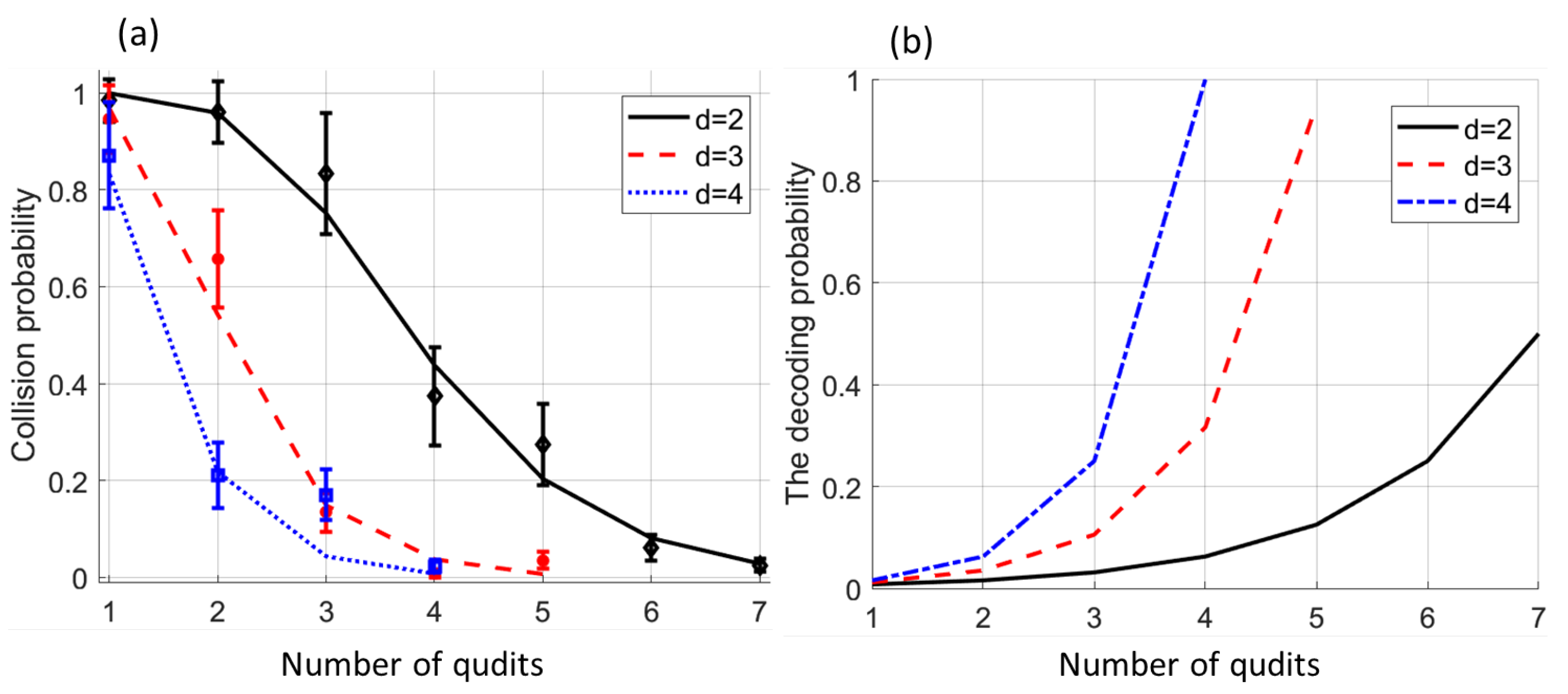
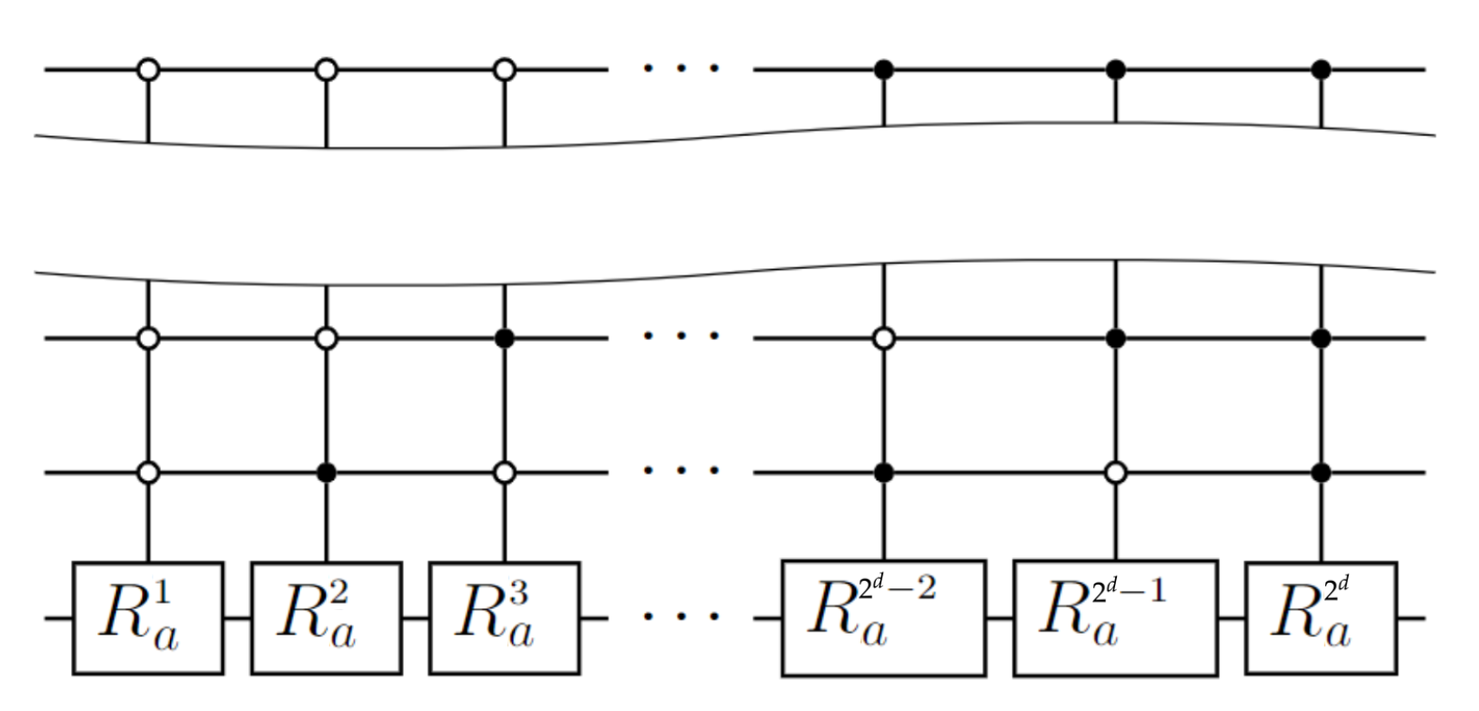

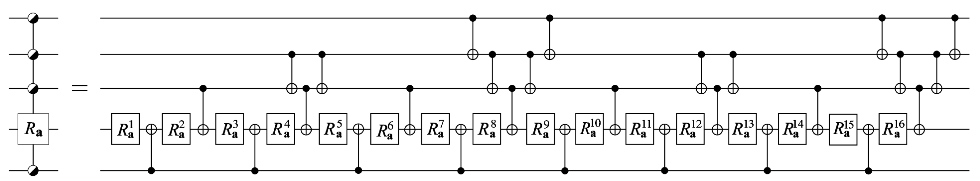
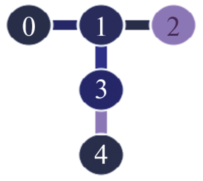
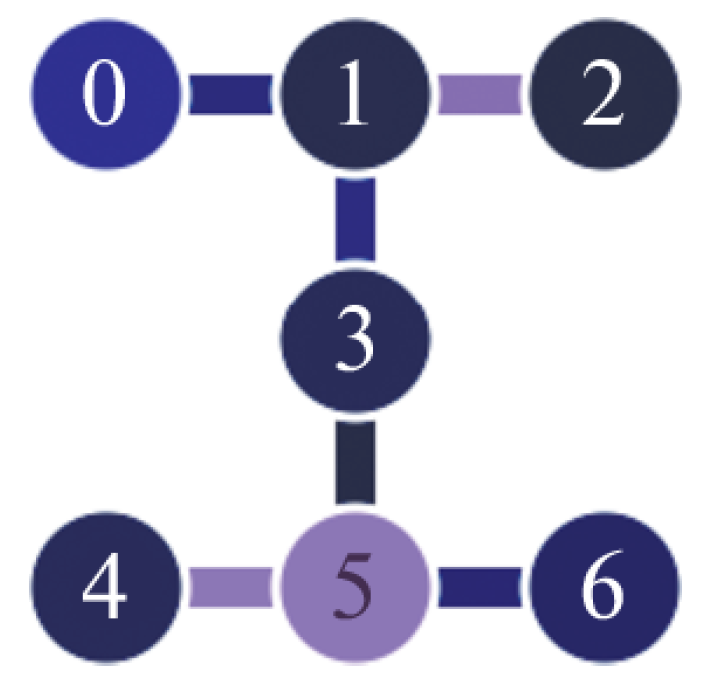
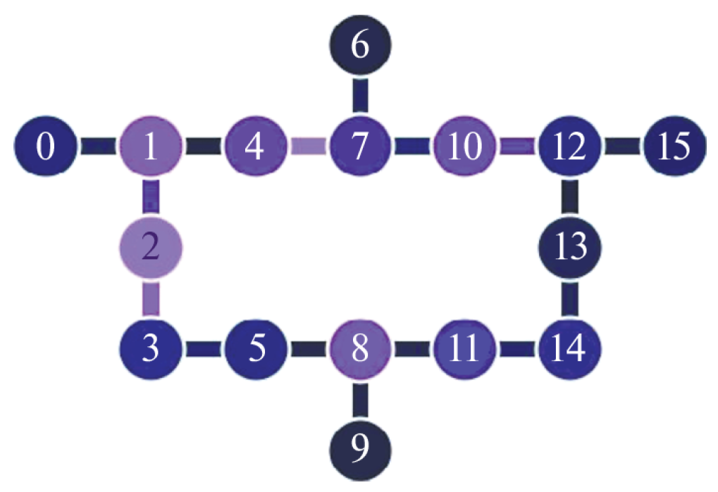
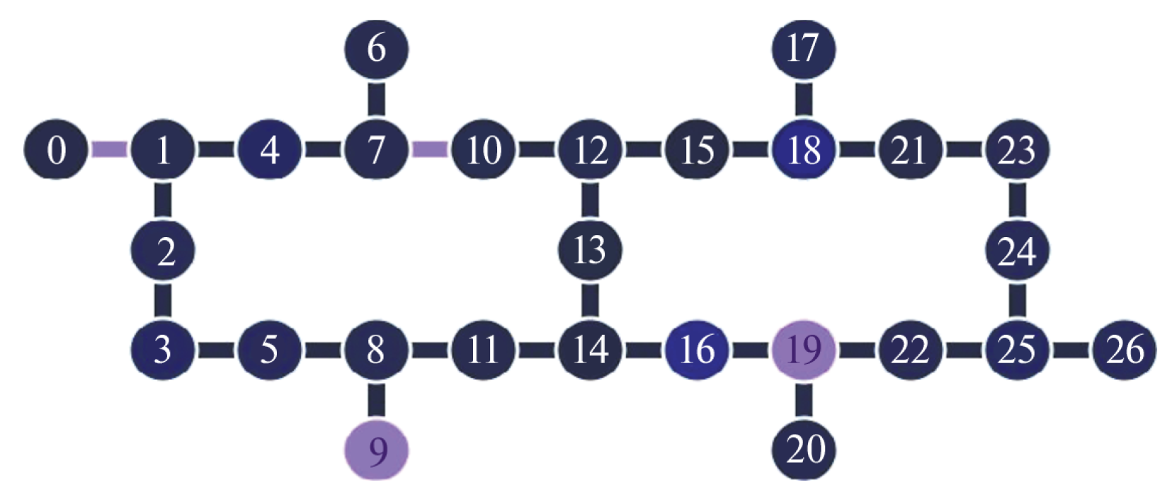
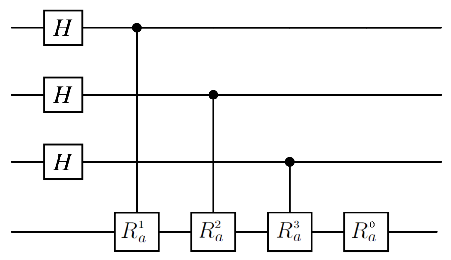
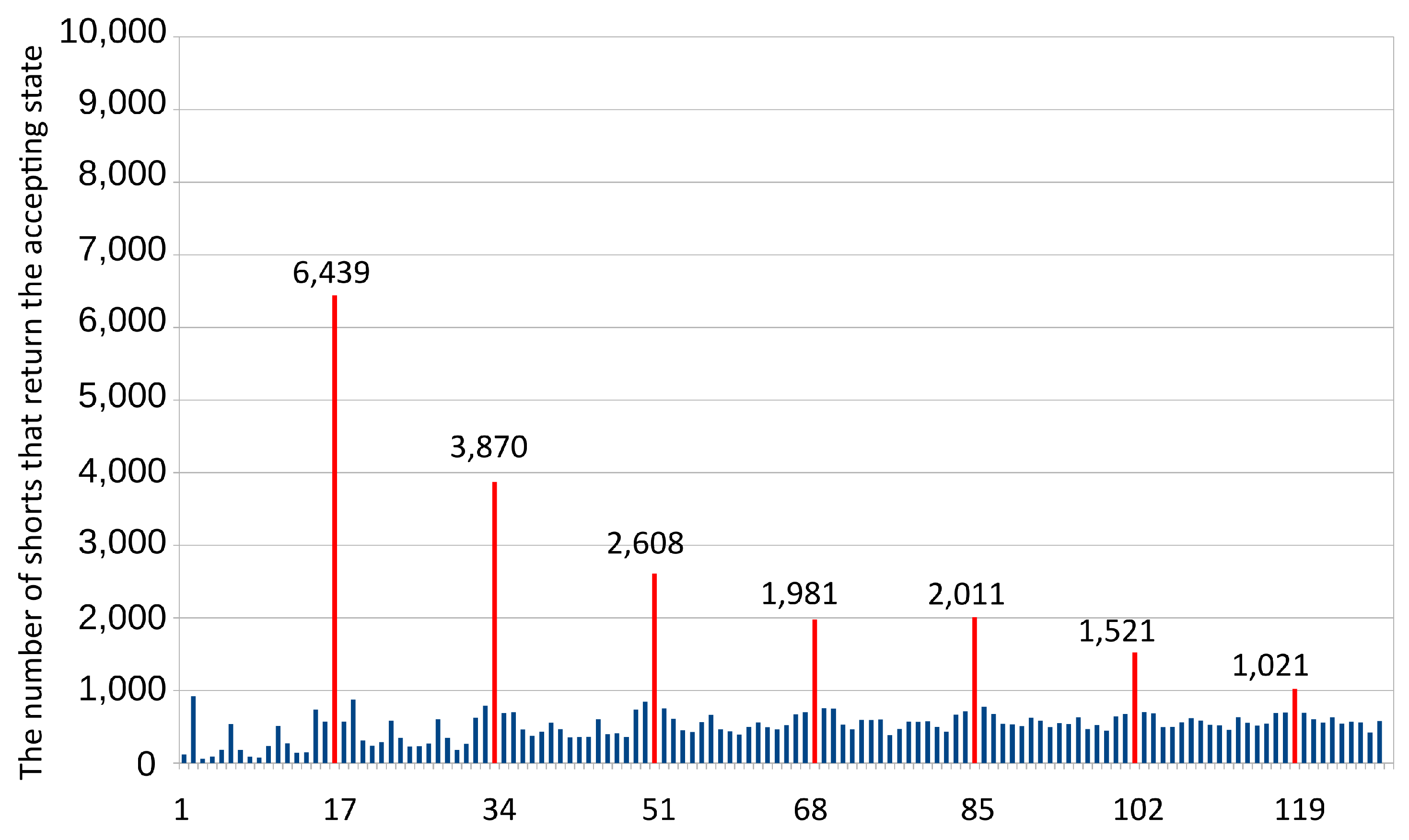


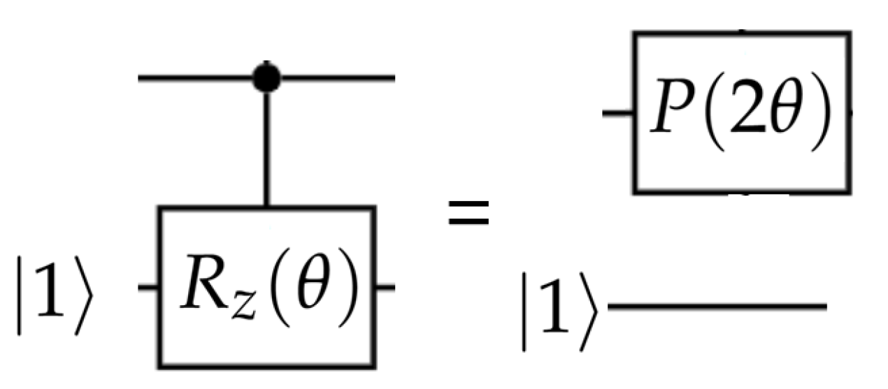
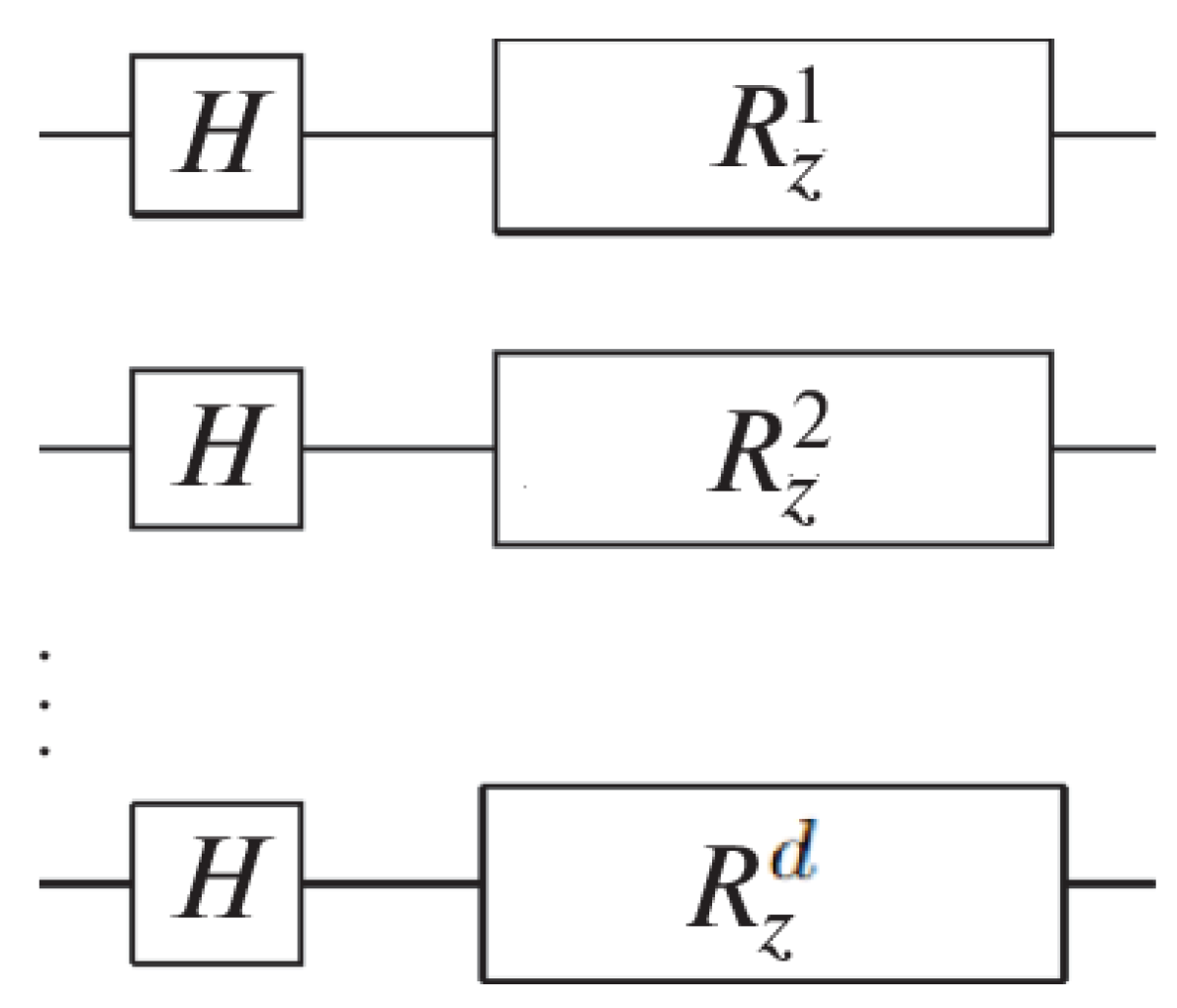
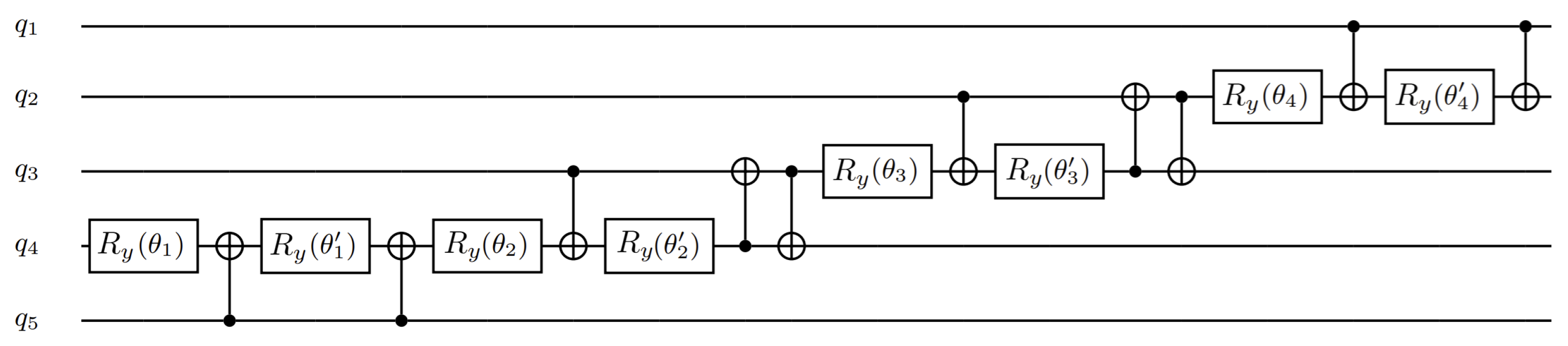

Disclaimer/Publisher’s Note: The statements, opinions and data contained in all publications are solely those of the individual author(s) and contributor(s) and not of MDPI and/or the editor(s). MDPI and/or the editor(s) disclaim responsibility for any injury to people or property resulting from any ideas, methods, instructions or products referred to in the content. |
© 2025 by the authors. Licensee MDPI, Basel, Switzerland. This article is an open access article distributed under the terms and conditions of the Creative Commons Attribution (CC BY) license (https://creativecommons.org/licenses/by/4.0/).