Developing and Analyzing the Defect-Based Surface Codes Using Optimization Algorithms

Abstract

Fault tolerance is crucial for enabling large-scale quantum computations, with surface codes emerging as prominent error correction techniques due to their high error threshold and reliance on nearest-neighbor interactions. Despite the advantages of surface codes, they demand a substantial number of qubits to encode a single logical qubit, making them resource-intensive. Two primary approaches exist to encode multiple logical qubits: patch-based and defect-based. This study focuses on the latter approach, which involves creating holes in the surface code for logical qubit encoding. With the defect-based approach, we need to account for trade-offs between the number of logical qubits and the logical error rates, so we employ an optimization algorithm to evaluate the maximum number of logical qubits for a given error rate. Through a series of experiments, we assess the limitations of the defect-based approach and investigate the impact of various hole types on logical qubit encoding.

1. Introduction

Quantum computing (QC) devices apply the principles of quantum physics to perform calculations that are impossible or very slow for classical computers. One major advancement in the past decade was the introduction of the Noisy Intermediate-Scale Quantum (NISQ) era by John Preskill in 2018 [1]. This period will continue for several years, until more scalable and resilient quantum technologies are developed. NISQ computers feature quantum processors with a limited number of qubits that are not large enough to achieve quantum supremacy or fault tolerance. Despite their limitations, NISQ devices can perform tasks beyond classical computers’ capabilities, including simulating quantum systems [2], optimizing complex problems, and exploring quantum machine learning [3,4]. NISQ devices are susceptible to errors, making them a valuable asset for investigating error reduction and resilience techniques. These techniques can potentially reduce errors in quantum computations, thereby enhancing their reliability and precision.

Since 1995 [5], several studies on quantum error correction (QEC) methods have been developed. Some known techniques provide error protection, such as quantum error correction codes [6,7,8], decoherence-free subspaces [9], and dynamical suppression of decoherence [10]. QC faces limitations in employing classical error correction techniques, including the no-cloning theorem, destroying superposition after error measurement, and diversity of errors. To overcome these problems, most QEC codes, such as the CSS (Robert Calderbank, Peter Shor, and Andrew Steane) [11] code and topological codes [12] like surface codes [13], are described in terms of stabilizer codes [14]. Most QEC codes use syndrome measurements to detect and correct errors without disturbing the encoded state.

The surface code is gaining attention as a potential method for fault-tolerant quantum computation [15] because of its inherent resilience against errors. There are various kinds of surface codes that differ based on the shape and boundary conditions of the lattice. For example, the toric code [16] represents a surface code on a torus-shaped lattice with periodic boundary conditions and encodes two logical qubits. In contrast, the planar code represents a single logical qubit on a square lattice with open boundary conditions. Although less efficient than the toric code in terms of logical qubit encoding, the planar code [17] is more practical and compatible with current technologies due to its lack of periodic boundaries. Despite its potential for fault-tolerant quantum computation, the practical implementation of the surface code still faces challenges. It demands many physical qubits to encode each logical qubit, thus reducing the efficiency and scalability of the quantum system. Additionally, increasing the size or distance of the lattice in the surface code does not lead to more logical qubits.

Several different methods are available to encode multiple logical qubits. Patch-based encoding stands out as one of the most prominent approaches. Patch-based encoding [18,19] employs multiple surface code patches, each representing one logical qubit. It resembles the classical approach for increasing bit width in computers by adding bits or wires. However, to enable interaction between different patches or tiles and build multiple qubit gates, the patches must undergo lattice surgery. The lattice surgery [20] consists of two operations: merging and splitting patches. The iterative application of the merging and splitting procedure leads to interaction between qubits, thus enabling operations with multiple qubits, like Controlled NOT (CNOT). However, lattice surgery requires redundant patches to build multiple qubit gates, thus lowering surface code density.

An alternative to the patch-based approach is the defect-based method, which removes the need to add multiple surface code patches. Instead, encoding multiple qubits is performed by removing specific stabilizers in one lattice [21,22]. In graph representation of surface code, stabilizers correspond to vertices and faces. Thus, we can increase the number of logical qubits by introducing gaps or holes in the surface code [8]. However, it is essential that the omitted stabilizers remain independent from one another and from the boundaries of the lattice. If they are not independent, they will not expand the dimension of the logical subspace, meaning they cannot encode additional logical qubits. Adding gaps in a surface code can increase the number of logical qubits, but it also raises the logical error rate of encoded qubits because some stabilizers are omitted. Thus, there is a trade-off between increasing the logical qubit count and controlling the associated error rates.

This study examines the benefits and limitations of a defect-based approach for encoding multiple logical qubits. We aim to assess the density of encoding logical qubits of surface codes in a defect-based approach while maintaining desired logical error rates. As the relationship between the defects in surface code and error rates is complex, we approach it as an optimization problem. For this aim, we employ the simulated annealing and genetic algorithms to place defects in the surface code lattice. At the same time, we use Squab [23] to evaluate logical error rates and quantify the number of logical qubits in surface codes for a chosen set of defects. By combining optimization methods with precise error rate analysis from Squab, we plan to identify the limitations of a defect-based approach for encoding multiple logical qubits.

Significant effort has been devoted to finding optimal methods for encoding quantum bits. One related approach, developed by Nautrup et al. [24], employs a reinforcement learning method to reduce the logical error rate by adding physical qubits to a standard square lattice. At the heart of their solution is a reinforcement framework that customizes the surface code to account for realistic noise. Similar to our approach, they use Squab to evaluate the error rates of the modified lattice. However, their approach focuses on achieving a desired logical error rate rather than addressing the challenges associated with encoding multiple logical qubits. In contrast, our approach follows the work in [8], which addresses the encoding of multiple qubits by inserting defects into surface codes. Although the study in [8] outlines the theoretical foundations and potential advantages of defect-based encoding, it lacks a comprehensive analysis of how scaling the number of logical qubits influences logical error rates. Our work aims explicitly to fill this gap by employing optimization algorithms to address the trade-off between logical qubit density and error performance. By employing a different multi-qubit encoding scheme, our work can be seen as complementary to the approach presented in [24].

This paper is organized as follows. Section 2 briefly introduces the most important concepts of quantum errors, error thresholds, noise channel, and surface code. Section 3 details the proposed method, which employs optimization algorithms, including SA and GA. In Section 4, we present our findings on the optimal placement of holes in surface codes and the impact of code distances on error characteristics. Section 5 provides a critical discussion of the advantages and limitations of the defect-based encoding approach. Finally, Section 6 offers our conclusions.

2. Backgrounds

2.1. Quantum Errors

A noise model in quantum is a mathematical description of how noise affects a quantum system or a quantum computation. Noise can originate from various sources, such as decoherence, faulty gates, measurement errors, crosstalk, and other sources [25].

The operator-sum representation is useful for analyzing and simulating noise and decoherence and designing quantum error correction codes and fault-tolerant quantum computation schemes. The operator-sum representation describes a quantum operation or channel that acts on a quantum system. It is also known as the Kraus representation [26]. The idea is to express the quantum operation as a sum of operators that act on the system, such that the final state is obtained by applying each operator to the initial state and then taking the partial trace over the environment. We start by considering a principal system to which an environment system is adjoined. This environment system is presumed to be spanned by an orthonormal set of basis states, denoted as $|e_i\rangle$, where $1\le i\le d^2$. The environment system is initially prepared in a pure state, $\left|e_0\rangle \langle e_0\right|$. In addition, the environment and initial state are originally uncorrelated. The operator-sum representation is described as the following [27]:

$$\begin{array}{ll}\epsilon (\rho )& =t{r}_{env}[U(\rho \otimes |e_0\rangle \langle e_0|)U^{†}]\hfill \\ & ={\displaystyle \sum _i\langle e_i|U(\rho \otimes |e_0\rangle }\langle e_0|U^{†}|e_i\rangle \hfill \\ & ={\displaystyle \sum _i{E}_i\rho E_i^{†}}\hfill \end{array}$$

(1)

where $\rho$ is the initial state of the system, and $U$ is a unitary operation to the joint state. $E_i, 1\le i\le d^2$ are the operators that represent the effect of the environment, and $\epsilon \left(\rho \right)$ is the final state of the system. The operators, $E_i$, must satisfy the completeness relation:

$${\displaystyle \sum _i{E}_i^{†}}{E}_i=I$$

(2)

where I is the identity operator. This ensures that the quantum operation preserves the trace of the state; that is, $tr\left(\epsilon \left(\rho \right)\right)=tr\left(\rho \right)$.

It has been shown that the overall effect of noise is modeled in terms of a set of Pauli operators and the identity acting on the physical qubits. The Pauli-X error flips the quantum state (bit-flip error), the Pauli-Z error flips the sign ($\alpha \left|0\rangle +\beta \right|1\rangle \to \alpha \left|0\rangle -\beta \right|1\rangle$) (phase-flip error), and the Pauli-Y error is a combination of the Pauli-X and the Pauli-Z errors at the same time (bit- and phase-flip error) [28].

2.2. Threshold Error and Noise Channel

The quantum threshold theorem asserts that using QEC codes, a quantum computer with a physical error rate below a specific threshold can reduce the logical error rate to arbitrarily low levels. In other words, the threshold of a topological code, $P_{th}$, is the maximum physical error; if the amount of physical error is less than that $P<P_{th}$, the logical error rate can be significantly reduced by increasing the size of the surface code [29]. The threshold of a code depends on the noise model and decoder; there is not a single threshold for a given QEC code.

Numerous noise models exist, with the most prominent being depolarizing and erasure channels. The quantum depolarizing channel [30] is traditionally used for quantum noise models in quantum systems. The depolarization channel, a quantum operation, changes the input qubit to a completely random state. The depolarization channel maps a state onto a linear combination of itself and the maximally mixed state, ${\displaystyle \frac{1}{d}}$, where d is the dimension of the system. The receiver does not know which qubits have been affected by the noise in the depolarization channel. On the other hand, the quantum erasure channel [31] is a quantum channel that replaces the incoming qubit with an “erasure state” ∣2⟩ orthogonal to both ∣0⟩ and ∣1⟩, with probability ϵ. Consequently, the receiver is informed that it has been erased. The erased qubit is replaced by a maximally mixed state in the erasure channel. It is equal to considering the qubit is exposed to a random Pauli error selected uniformly.

Our choice of the erasure channel with a probability of p = 0.1 for benchmarking surface codes requires justification. We deliberately selected this noise model based on computational efficiency considerations. As described by Delfosse et al. [23], the erasure channel provides substantial computational savings compared to the depolarizing channel while still sharing many general trends and features with more complex noise models. The erasure probability of 0.1 was selected to be below the theoretical erasure threshold for surface codes under error-free syndrome extraction, which is approximately 0.5 [32], but high enough to meaningfully differentiate between different code configurations. This approach follows the strategy outlined in the Squab framework: quickly identifying promising code configurations that can later be subjected to more expensive and detailed simulations with more complex noise models.

2.3. Surface Code

Surface codes represent quantum error correction codes that use a lattice of qubits to encode and manipulate logical qubits. The surface code introduced by Kitaev [16] is based on the stabilizer code, which employs syndrome measurements to detect errors without destroying data qubits. A stabilizer code is a class of QEC code that uses a stabilizer group, an Abelian subgroup of the Pauli group, to encode quantum states. Any Abelian group of Pauli operators defines the subspace of the Hilbert space:

$$C(\varsigma )=\left\{|\psi \rangle |{\varsigma }_i|\psi \rangle =|\psi \rangle ,\forall {\varsigma }_i\in \varsigma \right\}$$

(3)

$k$ logical qubits are encoded into n physical qubits by the stabilizer when $\varsigma$ has $n-k$ stabilizer generators. The stabilizer detects errors when ${\varsigma }_i\in \varsigma$ anticommutes with error $E$.

$${\varsigma }_i\left(\epsilon \left(|\psi \rangle \right)\right)=-\epsilon {\varsigma }_i|\psi \rangle =-\epsilon |\psi \rangle$$

(4)

So, the eigenvalue of $\epsilon |\psi \rangle$ is −1 for the stabilizer ${\varsigma }_i$. If the error operator commutes with each element of the stabilizer group, the error cannot be detected, because the eigenvalue of the operator from the stabilizer is +1. Therefore, if all the possible errors have unique error syndromes, we can correct the set of errors.

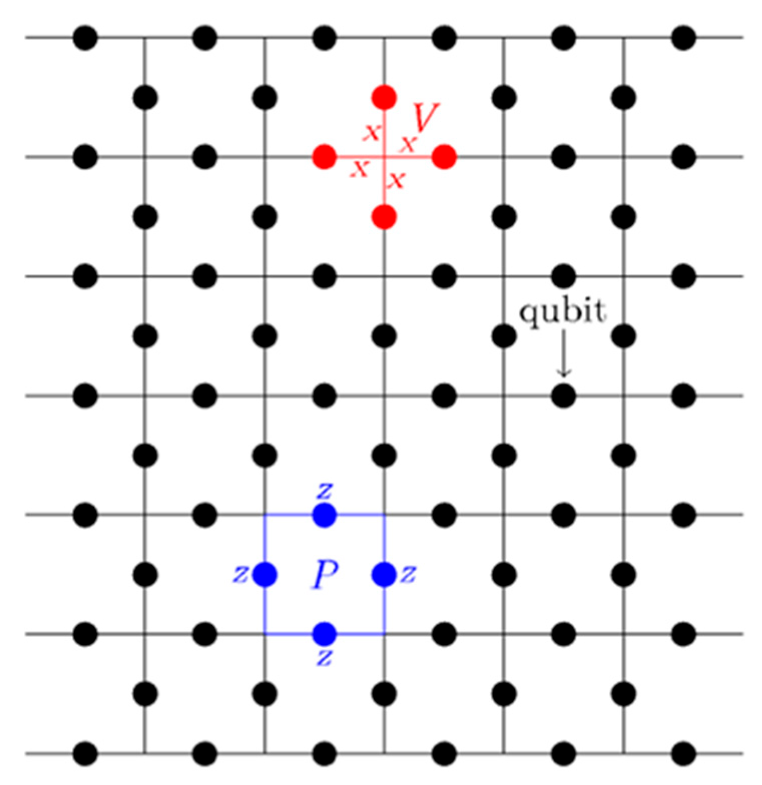
There are two types of stabilizer generators: a Z stabilizer for detecting X errors and an X stabilizer for detecting Z errors. In the planar surface code with a finite lattice, the X stabilizers are placed where the vertices are, while the Z stabilizers correspond to faces (plaquettes). A planar surface code with two different types of boundary conditions is illustrated in Figure 1, where the dots represent physical qubits. The boundary of the face, marked by four blue-colored edges, shows a Z stabilizer ($Z_p$), and the red-colored edges depict an X stabilizer ($X_v$), and both are defined by Equation (5):

$$X_v={\displaystyle \prod _{i\in vertex(v)}{X}_i\mathrm{and}{Z}_p={\displaystyle \prod _{i\in Boundary(p)}{Z}_i}}$$

(5)

where $X_v$ is the product of the Pauli X operators acting on the qubits and, $Z_p$ is a product of the Pauli Z operators. Vertex (v) and plaquette (p) have either 0 or 2 common edges, so these operators, $X_v$ and $Z_p$, commute with each other. If the lattice is $n\times m$ in size, it has nm vertical edges and $\left(n+1\right)\left(m+1\right)$ horizontal edges, equaling $2nm+n+m+1$ physical qubits [13]. In this lattice, there are $n\left(m+1\right)$ face (Z) stabilizer operators and $\left(n+1\right)m$ vertices (X) stabilizer operators. With $2nm+n+m+1$ qubits and $2nm+n+m$ independent stabilizer operators, the lattice has $\left(2nm+n+m+1\right)-\left(2nm+n+m\right)=1$ degrees of freedom, meaning that only one logical qubit may be encoded.

As mentioned above, $X_v$ and $Z_p$ detect Z error and X error, respectively. The quantum errors are detected by performing stabilizer measurements on groups of four qubits that form plaquettes and vertices on the lattice. These measurements can reveal whether a bit-flip or a phase-flip error has occurred on any of the qubits. The measurement outcomes form a syndrome, which is a classical bit string that indicates the type and location of errors. By repeating the stabilizer measurements over time, one can track the errors and correct them using appropriate decoder algorithms [33].

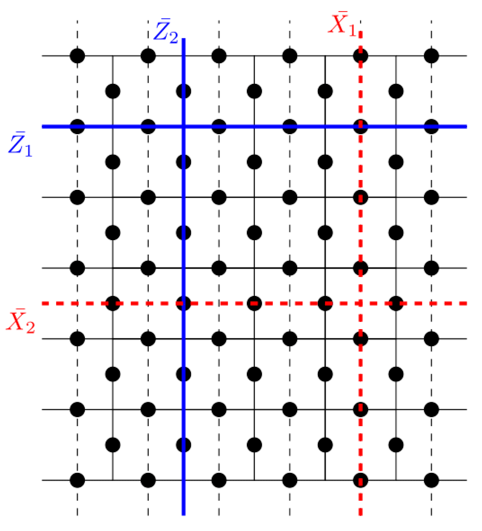
The number of quantum errors that can be identified and corrected is related to the minimum distance. The minimum distance in surface code is the size of the smallest non-trivial loop on the lattice. Non-trivial loops are related to the logical operators that act on the logical qubits. In the surface code, a logical operator, a set of Pauli operators, commutes with all the stabilizers of the code while acting non-trivially on the logical qubits. The logical operators are different depending on the geometry and boundary conditions of the lattice. The logical operators commute with all stabilizers. For example, in a surface code defined on a planar lattice, the logical Z operators, shown as red lines in Figure 2, form a subset of edges. The logical X operators, depicted as blue lines, are defined in a dual lattice, which is illustrated by the dashed lines in Figure 2. The distance of the surface code is the minimum size of a logical operator. In a lattice of dimensions $n\times m$ with an open boundary, the minimum distance is given by $d=min\left\{n+1, m+1\right\}$. The code is capable of protecting against $\left(d-1\right)/2$ errors.

2.4. Determining the Number of Logical Qubits with Holes

In this section, we provide more details about the planar lattice and its dual lattice concepts to define the general surface code with open and closed boundaries. In the paper [8], a compact 2-manifold S is cellulated to create a surface code. The surface code is represented as a triple $\left(V,E,F\right)$, and within this triple is a finite graph known as $G=\left(V,E\right)$, where each connected component of $S\backslash G$ is a disk corresponding to a face $f\in F$ of the cellulation. A face is considered a subset of $f\subset E$ because it is associated with the collection of edges on its boundary. If an edge of G is incident to just one face of G, it is defined as a boundary edge. In the generalized surface code, each edge on the boundary can be either open or closed. A face with a boundary edge is called a boundary face, denoted as $\partial F$. The boundary vertices, $\partial V$, are the endpoints of boundary edges, $\partial E$. The indices $C$ and $O$ stand for non-open (closed) and open components of the surface code. For instance, the sets of non-open (closed) vertices, edges, and faces are denoted by $V_C$, $E_C$, and $F_C$, respectively. The number of connected components of G containing no closed boundary edge is denoted by ${\kappa }_{\overline{{\partial }_{C}E}}\left(G\right)$, and the number of connected components of G containing no open vertices is denoted by ${\kappa }_{\overline{{\partial }_{O}V}}\left(G\right)$.

In Ref. [8], the dual surface code $G^{\ast }=\left(V^{\ast },E^{\ast },F^{\ast }\right)$ with open and closed boundaries is defined from $G=\left(V,E,F\right)$ by replacing each face $f\in F$ of G with a non-open vertex $V\backslash \partial V\in V^{\ast }$. Each closed edge, $e\in {\partial }_{C}E$, of G is substituted with an open vertex, ${\partial }_O{V}^{\ast }$. Non-open edges, E$\backslash \partial E\in E^{\ast }$, are obtained by connecting two vertices of G* if they correspond to distinct faces of G that share an edge. In addition, each edge, ${\partial }_{O}E\in E^{\ast }$, is acquired by connecting $V\backslash \partial V\in V^{\ast }$ and ${\partial }_O{V}^{\ast }$ if $V\backslash \partial V\in V^{\ast }$ corresponds to $f\in F$ is the unique face of G containing the boundary edge, e. Open edges, ${\partial }_O{E}^{\ast }$, are defined for every pair of distinct closed boundary edges, ${\partial }_{C}E$, sharing a closed boundary vertex, $vϵ{\partial }_{C}V$, in G. A face from the cycle $F_v$ in G* for each $vϵV\backslash \partial V$ is defined as a non-open face, and a face from the cycle ${\overline{F}}_vϵ{\partial }_O{F}^{\ast }$ for each $vϵ{\partial }_{C}V$ is defined as an open face.

It can be concluded that the following bijection exists between the surface code $G=\left(V,E,F\right)$ and its duality, $G^{\ast }=\left(V^{\ast },E^{\ast },F^{\ast }\right)$

$$\begin{array}{l}F\leftrightarrow V^{\ast }\backslash \partial V^{\ast }\hfill \\ {\partial }_{C}E\leftrightarrow {\partial }_O{V}^{\ast }\hfill \\ E\backslash \partial E\leftrightarrow E^{\ast }\backslash \partial E^{\ast }\hfill \\ {\partial }_{C}V\leftrightarrow {\partial }_O{E}^{\ast }\hfill \\ V\backslash \partial V\leftrightarrow F^{\ast }\backslash \partial F^{\ast }\hfill \\ {\partial }_{C}V\leftrightarrow {\partial }_O{F}^{\ast }\hfill \end{array}$$

(6)

The generalized surface code $G=\left(V,E,F\right)$ with a block size n, representing the number of closed edges, $E\backslash {\partial }_{O}E$ (i.e., the number of physical qubits); k, the number of logical qubits encoded; and d, the minimum distance, is indicated as $⟦n,k,d⟧$. The following formula determines the number of logical qubits:

$$k=-\left|V_C\right|+\left|E_C\right|-\left|F\right|+{\kappa }_{\overline{{\partial }_{C}E}}\left(G\right)+{\kappa }_{\overline{{\partial }_{O}V}}\left(G\right)$$

(7)

The minimum code distance is the minimum length of a non-trivial relative cycle of G and G*. The non-trivial relative cycle of G that is denoted as $d_Z$ is the logical Pauli Z operator. Moreover, the logical Pauli X operator, d_X, is a non-trivial relative cycle of G*.

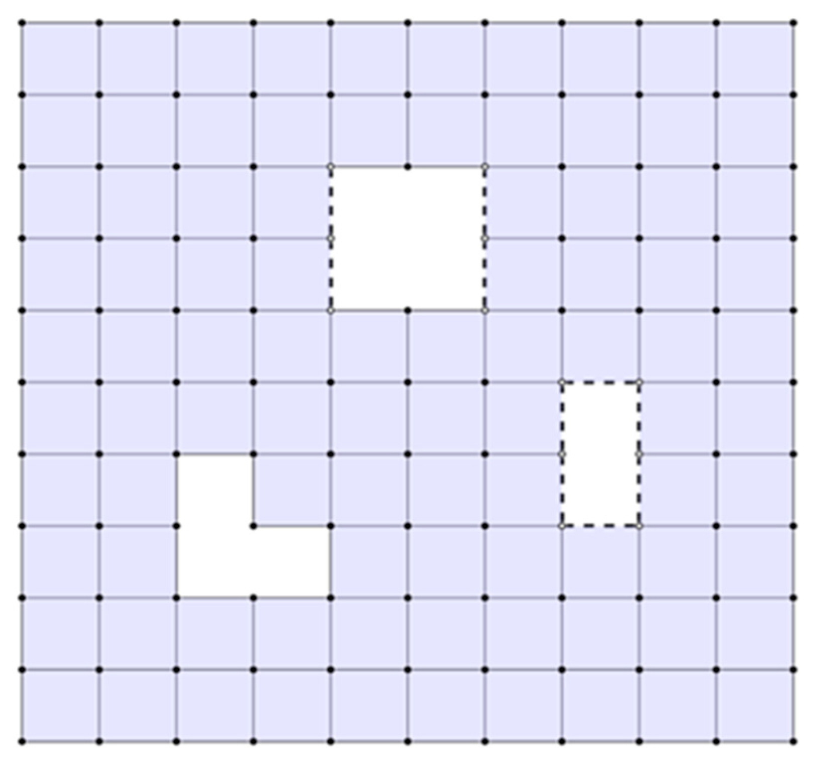
Figure 3 shows a surface code consisting of two closed holes (Ref. [8] considered the external boundary as a closed hole), one open hole, and one partially open hole. The number of closed edges in the surface code is 203, the number of closed vertices is 108, and the total number of faces is 91. Therefore, the number of logical qubits encoded is 4 by using Equation (7).

2.5. Maximum Possible Number of Logical Qubits with Closed Holes on a Square Lattice Surface Code of Dimensions n by n

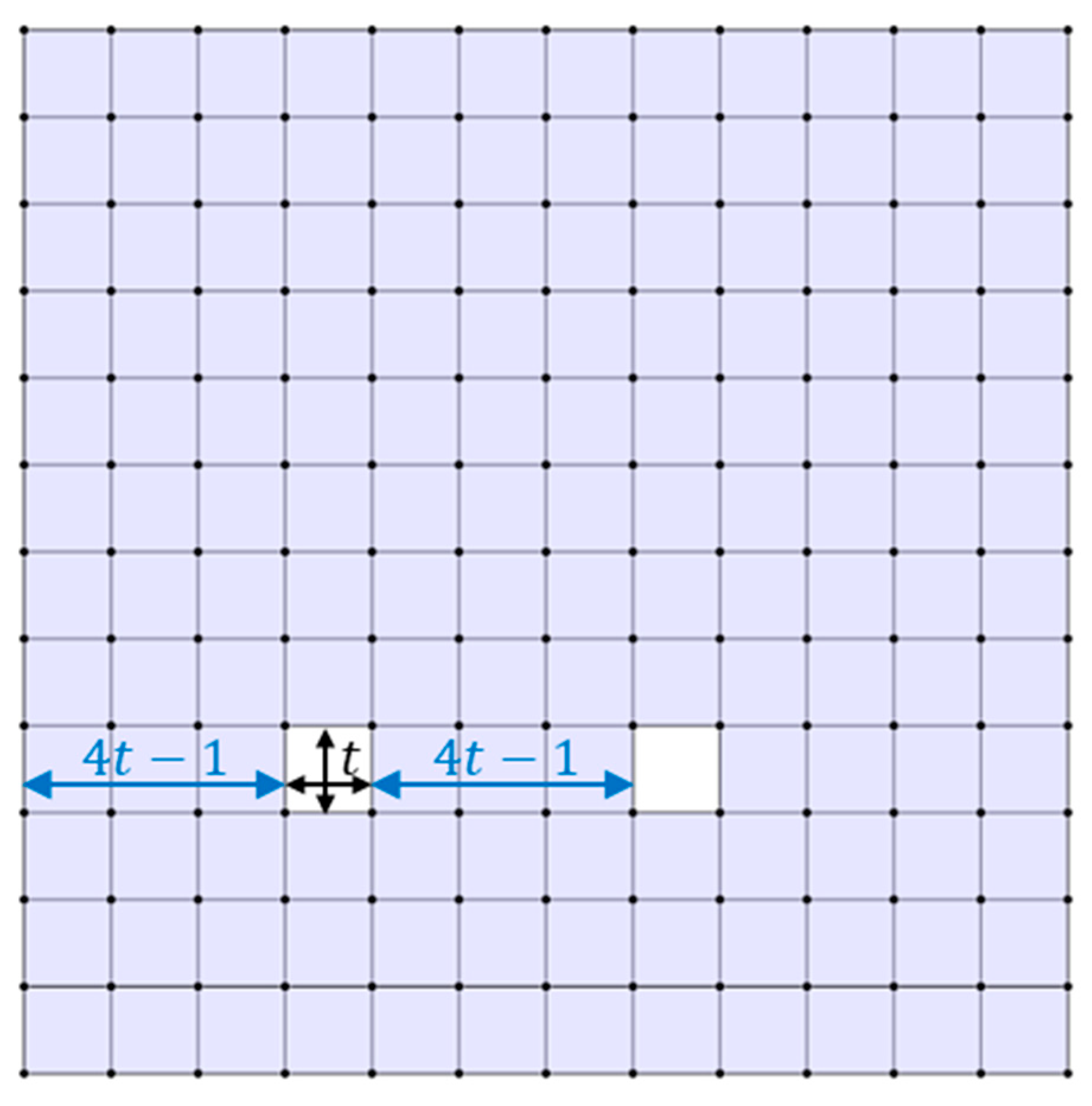
In [8], the method for calculating the minimum distance of a code in a square lattice surface code punctured with square holes is discussed. Each qubit corresponds to a closed hole of size $t\times t$, and these holes are separated from each other and from the boundary by $4t-1$. This separation ensures that the minimum distance of the code is $d=4t$. This lattice is depicted in Figure 4. For instance, if a hole is $1\times 1$ and the separation between holes and from the boundary is three, then the minimum distance of the code is four. If the distance between holes and hole and boundary are less than $4t-1$, then the minimum distance is less than $4t$ and is equal to this distance. 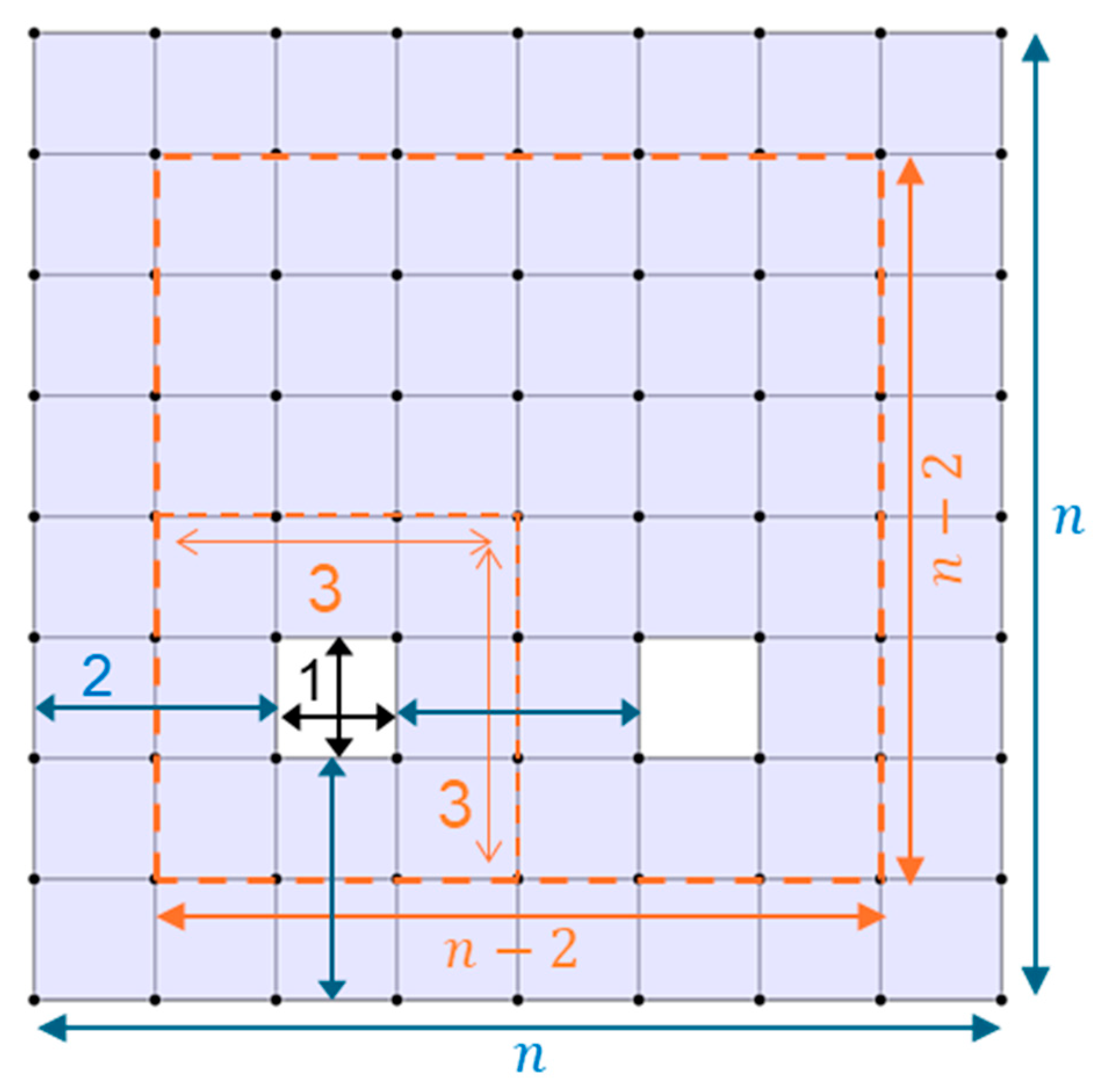As shown in Figure 5, if the holes are separated from each other and from the boundary by two, then the minimum distance of the code is three. The number of encoded qubits is determined by the number of closed holes. Therefore, the number of logical qubits achievable within a tile depends on the minimum distance of the code and the size of the hole. It can be said that if the minimum code distance is three, a hole consisting of one face is the optimal choice for maximizing space to create additional logical qubits.

To find the maximum number of holes that can be placed in a lattice while maintaining the minimum code distance of three, we consider a 3 × 3 square around each hole. Additionally, each hole should be at least two faces away from the boundary, which means that each 3 × 3 square should be placed within an (n − 2) by (n − 2) area, as shown in Figure 5. Assuming that the minimum code distance is three and the closed hole consists of one face, the maximum number of logical qubits can be calculated using the following equation:

$$\mathrm{maximum}\mathrm{number}\mathrm{of}\mathrm{logical}\mathrm{qubits}=\lfloor {\displaystyle \frac{n-2}{3}}\rfloor \times \lfloor {\displaystyle \frac{n-2}{3}}\rfloor$$

(8)

This formula can be used in any size of lattice. Additionally, if two boundaries of the lattice consist of open edges, one more logical qubit is added to Equation (8).

A surface code with the maximum number of encoded qubits may not maintain an acceptable logical error rate. To optimize the placement and the number of holes in order to achieve a desired logical error rate, it is necessary to employ optimization methods.

2.6. The Number of Logical Qubits with Partially Open Holes on a Square Lattice Surface Code of Dimensions n by n

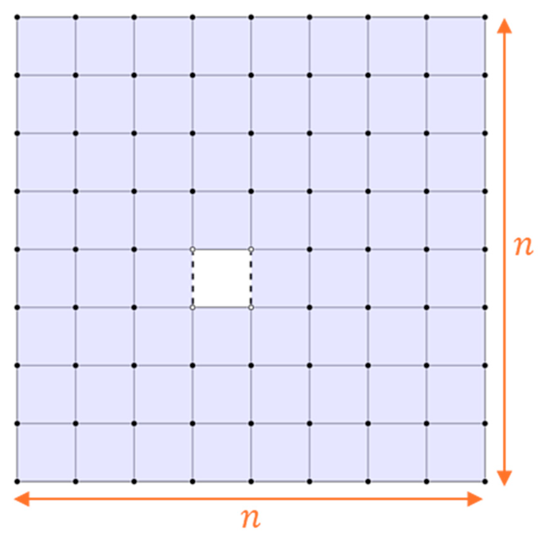
If a hole contains both open and closed edges, it is termed a partially open hole or mixed hole. As noted previously, a closed hole of any size increases the number of logical qubits by one. Therefore, the number of closed holes is directly proportional to the number of encoded qubits. In contrast, a partially open hole increases the count by more than one logical qubit. Consider a square lattice surface code punctured with a square hole having two open boundaries on each side; according to Equation (7), this results in two logical qubits. When two boundaries are open, the number of closed vertices decreases more compared to closed edges, thereby increasing the number of logical qubits, as determined by Equation (7). For instance, a square lattice n × n with a closed edge and closed boundary has one logical qubit because the lattice comprises $n^2-1$ faces, $\left(n+1\right)\times \left(n+1\right)$ closed vertices, and $2n\left(n+1\right)$ closed edges. Furthermore, the number of connected components of G containing no closed boundary edge is zero, and the number of connected components of G containing no open vertices is one. Therefore, the number of logical qubits is as follows:

$$\begin{array}{l}k=-\left|V_C\right|+\left|E_C\right|-\left|F\right|+{\kappa }_{\overline{{\partial }_{C}E}}\left(G\right)+{\kappa }_{\overline{{\partial }_{O}V}}\left(G\right)\\ k=-{(n+1)}^2+2n^2+2n-n^2+1+1\\ k=-n^2-2n-1+2n^2+2n-n^2+1+1=1\end{array}$$

(9)

If two boundaries of the hole are opened, as illustrated in Figure 6, the surface code consists of $n^2-1$ faces $2n^2+2n-3$ closed vertices, $2n^2+2n-2$ closed edges, and ${\kappa }_{\overline{{\partial }_{C}E}}\left(G\right)={\kappa }_{\overline{{\partial }_{O}V}}\left(G\right)=0$, resulting in the following count of logical qubits:

$$k=-n^2-2n+3+2n^2+2n-2-n^2+1=2$$

(10)

When two sides of a square hole are opened, this results in an increase in the number of open vertices by two compared to the number of open edges. Therefore, it can be concluded that two logical qubits are added when there is only one partially open hole. The first square partially open hole contributes two logical qubits, and each additional square partially open hole adds three more logical qubits, due to the reduction of one face, four closed vertices, and two closed edges. Consequently, the number of logical qubits with h partially open holes on a square lattice surface code of dimensions $n\times m$ is as follows:

$$k=2+3\times h$$

(11)

If the number of faces in a hole is more than one, it yields the same result as a hole with one face because, as the number of faces decreases, the number of edges also decreases.

Thus, a surface code with partially open holes leads to a substantial increase in the number of logical qubits.

2.7. Preserving Code Distance During Braiding

Logical operations in defect-based surface codes are often performed by braiding, which involves moving defects (holes) around each other to enact entangling gates such as CNOT [17,21]. One key advantage of this approach is that it does not require ancillary qubit patches as in patch-based lattice surgery. However, the movement of defects can dynamically alter their spacing and thus change the effective code distance. If defects are brought too close together during braiding, the minimum distance of logical operators may shrink, increasing the risk of logical errors [17,21]. Brown et al. [21] describe conceptual frameworks for preserving code distance during logical operations via careful control of defect trajectories and separation.

3. Proposed Method

In the context of surface codes, a standard lattice configuration with open edges and without holes encodes a single logical qubit. However, introducing holes into the surface code lattice can increase the number of encoded logical qubits while reducing resource overhead. This efficiency gain comes with a trade-off: as we introduce holes, the logical error rate tends to increase due to reduced code distance. To find an optimal balance between maximizing the number of encoded logical qubits and maintaining satisfactory error correction, we approach hole placements as a Knapsack problem [35].

The Knapsack problem is well-known in computer science and mathematics for its optimization challenge, particularly in combinatorial optimization. It has applications across various domains, like finance, logistics, and resource allocation, and serves as a fundamental problem in algorithm design and optimization studies. Finding an optimal solution is deemed NP-hard since there is no known polynomial-time algorithm for solving it, especially for large instances; however, several algorithms offer approximate solutions, such as SA (simulated annealing), genetic programming, and various heuristics suitable for real-world applications. In our scenario, we look at the surface code as a knapsack: the knapsack items symbolize the holes, we aim to introduce them in the code structure, and the weights of knapsack items represent the logical error rate that arises from presenting holes in the code. If inserting holes outweighs the desired logical error rate, we need to find another set of holes. Unlike traditional Knapsack problems, though, expressing the relationship between hole count/placement and logical error rate is challenging. Therefore, we rely on empirical assessment to determine the impact of the holes and their placement on the logical error rate, a task facilitated by the Squab framework.

The core idea of our method is illustrated in Figure 7. It employs a discrete optimization algorithm and the Squab framework. The discrete optimization algorithm predicts the best positioning of holes on the surface code, considering a specified logical error rate and selected constraints, which will be detailed later in this paper. The optimization algorithm interacts with the Squab process, which acts as an environment offering feedback through a logical error rate. If the error rate threshold is unmet, depending on the nature of the optimization algorithm, it will seek another subset of holes that meet the requirements for logical errors. Through an iterative process, our method explores potential solutions to maximize qubit numbers based on specific logical error demands.

Another viable approach for improving code density is patch-based or lattice concatenation. When surface codes are arranged adjacent, multiple codes can be combined to form a larger quantum computation [19,20]. However, incorporating holes in a surface code to encode more logical qubits in a lattice proves advantageous, enhancing the overall efficiency of the quantum computation process by reducing resource overhead, particularly in terms of fewer physical qubits, and optimizing error correction mechanisms. The strategic use of holes in the lattice allows for a more streamlined and resource-efficient implementation of large-scale quantum computing.

3.1. Maximizing the Number of Logical Qubits Using Optimization Algorithms

Expressing the loss function for determining the maximum number of logical qubits within a given logical error is difficult due to the intricate connection between hole placement and the rate of logical errors. Therefore, we rely on approximate algorithms to discover the optimal placement of holes in the lattice for a given logical error rate. Approximation algorithms play a crucial role in solving optimization problems, especially when finding an exact solution is computationally infeasible or too time-consuming. These algorithms provide solutions that are close to the optimal solutions, often within a provable bound, and are widely used in real-world applications where efficiency is a primary concern, e.g., manufacturing, placement of standard cells for chip design, finances, etc.

In the literature, a plethora of approximation algorithms exists to find near-optimal solutions for a given problem. Among the existing approaches, dynamic programming emerges as one of the widely embraced algorithms to tackle problems resembling Knapsack. However, when it comes to our problem, where we encounter a Knapsack-like situation, dynamic programming proves to be unviable. This is because the task of finding the perfect placement of holes cannot be simplified to the act of locating holes solely within subsections of the lattice. Simply concatenating these subsections in a naive manner within the lattice can lead to an undesirable increase in logical errors and significantly decrease the number of encoded logical qubits, as opposed to the effectiveness of locating holes across the entirety of the lattice.

3.1.1. Simulated Annealing

As an alternative to dynamic programming, we employ the simulated annealing (SA) approach [36] to find the optimal placement of holes in the lattice. SA is a probabilistic optimization technique inspired by the annealing process in metallurgy. It is used to find near-optimal solutions in complex search spaces by iteratively exploring the solution space. The temperature in SA plays a critical role in determining the algorithm’s behavior. The algorithm is more permissive at high temperatures, allowing it to explore a wide range of solutions, including those that may initially seem suboptimal. As the temperature decreases, the algorithm becomes more selective. The probability of accepting a worse solution is determined by the energy function and the current temperature, where solutions with smaller energy are optimal, and vice versa.

Its robustness and local search refinement make the SA a promising approach for finding the positions of holes that yield the maximal number of logical qubits. Additionally, its simplicity allows us to efficiently analyze even larger lattices. To adapt the SA to suit our requirements, we implemented several modifications. In our scenario, the solution space encompasses all potential arrangements of holes in a square lattice. The SA process commences with an open-boundary square lattice and a randomly selected hole. To generate neighboring solutions, we employ three distinct actions that are randomly chosen. The first action adds a new hole into the existing lattice in a random fashion. However, a hole must adhere to the selected code distance to be considered a viable candidate for generating neighboring solutions. Specifically, for a code distance of d, the holes in the lattice should be at least $d-1$ faces apart from themselves and the border of the lattice. The addition of holes can lead to poor error performance of the code.

Consequently, we have defined a second action: removing holes from the current solution. While the previous two actions alter the number of holes, the third action involves reassigning holes within the existing solution across the tiles to find a placement with a lower logical error rate. To evaluate potential solutions, we defined the following energy function:

$$E=e^{-N_Q}+E_{error}$$

(12)

where $N_Q$ represents the number of encoded logical qubits, and $E_{error}$ is defined as (13):

$$E_{error}=\{\begin{array}{cc}\alpha (LER-T_{LER}),\hfill & \hfill \left|LER-T_{LER}\right|<\epsilon \\ \beta (LER-T_{LER}),\hfill & \hfill otherwise\end{array}$$

(13)

LER represents the obtained logical error rate for the current solution; $T_{LER}$ represents the desired logical error rate for which we maximize the number of logical qubits; and alpha, beta, and script epsilon are real numbers, where beta is $\beta$ >> α. With the term $e^{-N_Q}$ in Equation (12), the SA favors the solutions that encode more logical qubits. However, with $\beta$ >> α in Equation (13), the SA penalizes solutions that deviate from desired logical error.

3.1.2. Genetic Algorithms

In addition to SA, we employed genetic algorithms (GAs) [37]. GAs are heuristic optimization techniques inspired by natural selection. The GA iteratively evolves the population over generations. It starts with an initial population, evaluates each individual’s fitness using the fitness function, and then uses selection mechanisms to choose individuals for reproduction, favoring those with higher fitness scores. The GA begins with lattices with one randomly selected hole and adds more through crossover and mutation. Crossover and mutation operators are applied to create a new population, which replaces the old one. This process continues until a termination condition, such as a maximum number of generations or a satisfactory fitness level, is met. During the crossover operation, we exchange two holes between the parent tiles. In the mutation operation, we introduce changes in a tile by adding or removing holes, resulting in a diversified solution space. As with the SA method, inserting new holes in the lattice must adhere to the code distance criterion. As we tackle the single-objective optimization problem, we employ classical steady-state criteria for selecting parents (SSGA) for its simplicity. The other widely used GA, NSGA-II, aims to solve multi-objective optimization problems, which is not the case in our paper. GAs have been successfully employed across domains such as bioinformatics, engineering, economics, and artificial intelligence to uncover optimal or near-optimal solutions. They are particularly effective when searching for solutions in large and complex solutions or when dealing with problems that lack a straightforward analytical solution, as is the case with the problem at hand. We use the following fitness function to quantify the quality of solutions in the iteration or generation of the single-objective optimization with GA:

$$E=N_Q+E_{error}$$

(14)

where $N_Q$ represents the number of encoded logical qubits, and $E_{error}$ is defined as follows:

$$E_{error}=\{\begin{array}{ll}\alpha (LER-T_{LER}),\hfill & \hfill \left|LER-T_{LER}\right|<\epsilon \\ \beta (LER-T_{LER}),\hfill & \hfill otherwise\end{array}$$

(15)

where LER represents the obtained logical error rate for the current solution; $T_{LER}$ represents the desired logical error rate for which we are maximizing the number of logical qubits; and $\alpha$, $\beta$, and $\epsilon$ are real numbers, where α >> $\beta$. The term $N_Q$ in Equation (14) enables the GA to select individuals in the population, corresponding to surface codes with more logical qubits. Moreover, with α >> $\beta$ in Equation (15), the GA rewards the individual surface codes, which exhibit logical error rates close to the desired one.

3.1.3. Squab

Squab (version 1.2) is software capable of constructing and displaying various lattice tilings and running fast Monte Carlo simulations to estimate error thresholds and logical error rates for different architectures. Several tools are available for simulating and decoding surface codes, including Stim and Qsurface. However, most of these tools lack native support for creating holes in the codes. Even when adding this functionality to a library is possible, the implementation can be complex. Squab is specifically designed for general 2D surface codes that simplify creating holes with open and closed boundaries in any shape. It was developed by Nicolas Delfosse et al. [23]. Squab utilizes the erasure channel, achieving greater computational savings compared to the depolarizing channel. It operates on the principle that the main difference between an erased and a depolarized qubit is the known location of the erasure. Squab assumes the decoding algorithm is aware of the erased qubits’ locations, which are typically measurable in experimental setups. Decoding stabilizer codes in this channel requires solving a linear system with generally cubic complexity. For generalized surface codes, Squab achieved a linear time benchmark by employing induced homology [23]. The software estimates errors by determining the correctability of an erasure for the surface code associated with surface G, its dual G*, and an erasure error. Squab supports any 2D planar lattice in any shape, with or without holes, and with open or closed boundaries. Additionally, it generates a performance report detailing the surface code’s features, the distribution of necessary measurements, and plots of the logical error rate after decoding X-error, Z-error, and both errors simultaneously.

As previously indicated, Squab provides feedback in the form of a logical error rate and the number of logical qubits encoded. It takes hole placements as input, generates a lattice with holes, and outputs code properties such as the logical error rate and the number of encoded logical qubits computed based on Equation (7). In the experiments that were conducted, we considered the logical error rate when the surface code was subjected to an erasure channel with an erasure probability of $p=0.1$. The selected probability is lower than the error threshold in the surface code under error-free syndrome extraction [32]. Furthermore, in the Squab, we performed 10,000 trials to assess the error of the designed quantum error correction code.

It is important to acknowledge that Squab’s erasure channel model assumes immediate and perfect knowledge of erasure locations, thus representing an idealization compared to physical hardware implementations. In real quantum systems, detecting qubit erasures (such as leakage events) requires additional measurement circuits and resources. These detection mechanisms would introduce overhead in the form of time delays, additional qubits, and potential false positives/negatives in erasure detection. While our current benchmarking approach does not model these practical complexities, it provides valuable theoretical bounds on the performance of different hole configurations. The comparison between different surface code layouts remains valid within this theoretical framework, as all configurations are evaluated under the same idealized conditions. This approach allows us to efficiently explore the design space of defect-based surface codes before moving to more resource-intensive realistic noise simulations.

4. Results

4.1. Maximizing Number of Qubits for a Given Logical Error Rate

In the first set of experiments, we assessed the maximal encoding density of square surface codes. Here, we fix the code distance of the surface code to three. Each experiment was repeated five times to ensure statistical accuracy, and the results were expressed with the mean and standard deviation. For the SA approach, we selected the initial temperature of 2400 K, which exponentially decreases to 0.5 K across 1000 iterations to cover the entire search space. At each temperature, the acceptance ratio is determined by Boltzmann probability, where we set the Boltzmann constant to one. In GA [38], we set the size of the population to 200 and the number of generations to 1000. To produce offspring in each generation, 50 parents are selected to produce offspring in each generation using the steady-state criterion. The genome length equals the maximal number of logical qubits (8), so we can represent all the potential holes of the lattice. The initial population represents one randomly selected hole, and subsequent holes are introduced through crossover and mutation. Each crossover is followed by a mutation of the genome, which leads to diverse solutions. We observed the performance of our approach for a predefined set of logical errors (${10}^{-4}, {10}^{-3}, 5\times {10}^{-3}, {10}^{-2}$). 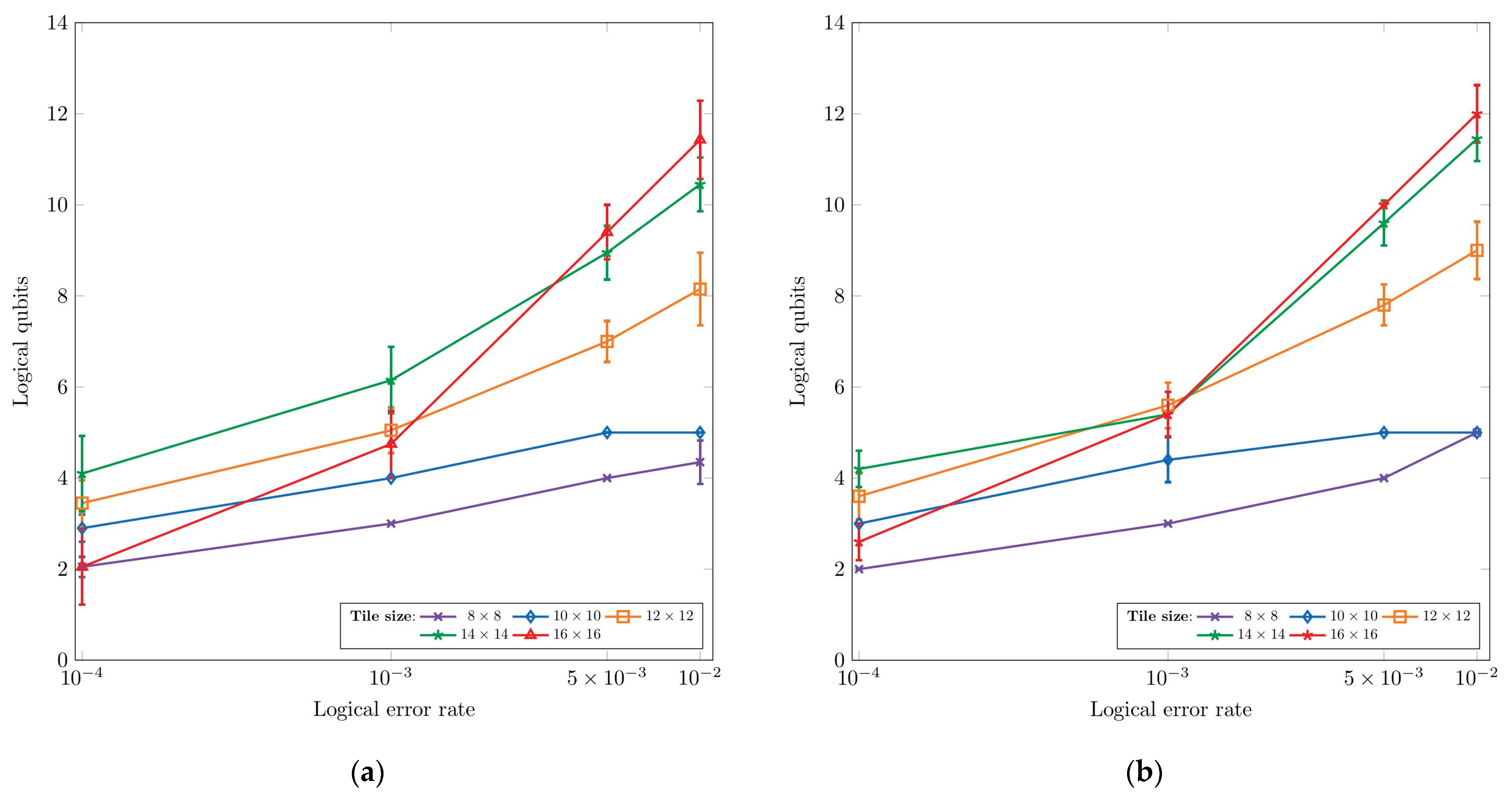In addition, we also assessed the behavior of the proposed solution for different sizes of the square lattice.

The results are presented in Figure 8a and Figure 8b for SA and GA, respectively. The y-axis represents the number of obtained logical qubits for the evaluated logical error rates on the x-axis per given tile size. As expected, we observe that we can encode more logical qubits with the increase in the logical error rate. Moreover, the tile size is crucial in obtaining more logical qubits. As discussed previously, smaller tiles yield fewer logical qubits due to constraints imposed by code distance. On the other hand, larger tiles enable the encoding of a higher number of logical qubits. Moreover, we can see that several tiles exhibit similar results for specific logical error rates. For example, all tiles exhibit a similar number of logical qubits for lower error rates, suggesting that we can employ smaller sizes and get the same number of logical qubits. By comparing results obtained from SA and GA, we can see that both methods deliver similar results, indicating the upper limits of the achieved number of logical qubits by inserting holes in the surface code lattice.

4.2. Evaluating Surface Codes with Partially Open Edges

In the previous section, we conducted experiments on holes with closed boundaries to determine the maximum number of qubits for a given logical error rate. This time, we investigate how holes with partially open edges affect the encoding density of surface code for a given logical error rate. Holes with partially open edges or partially open holes refer to holes with open, non-adjacent boundary edges. 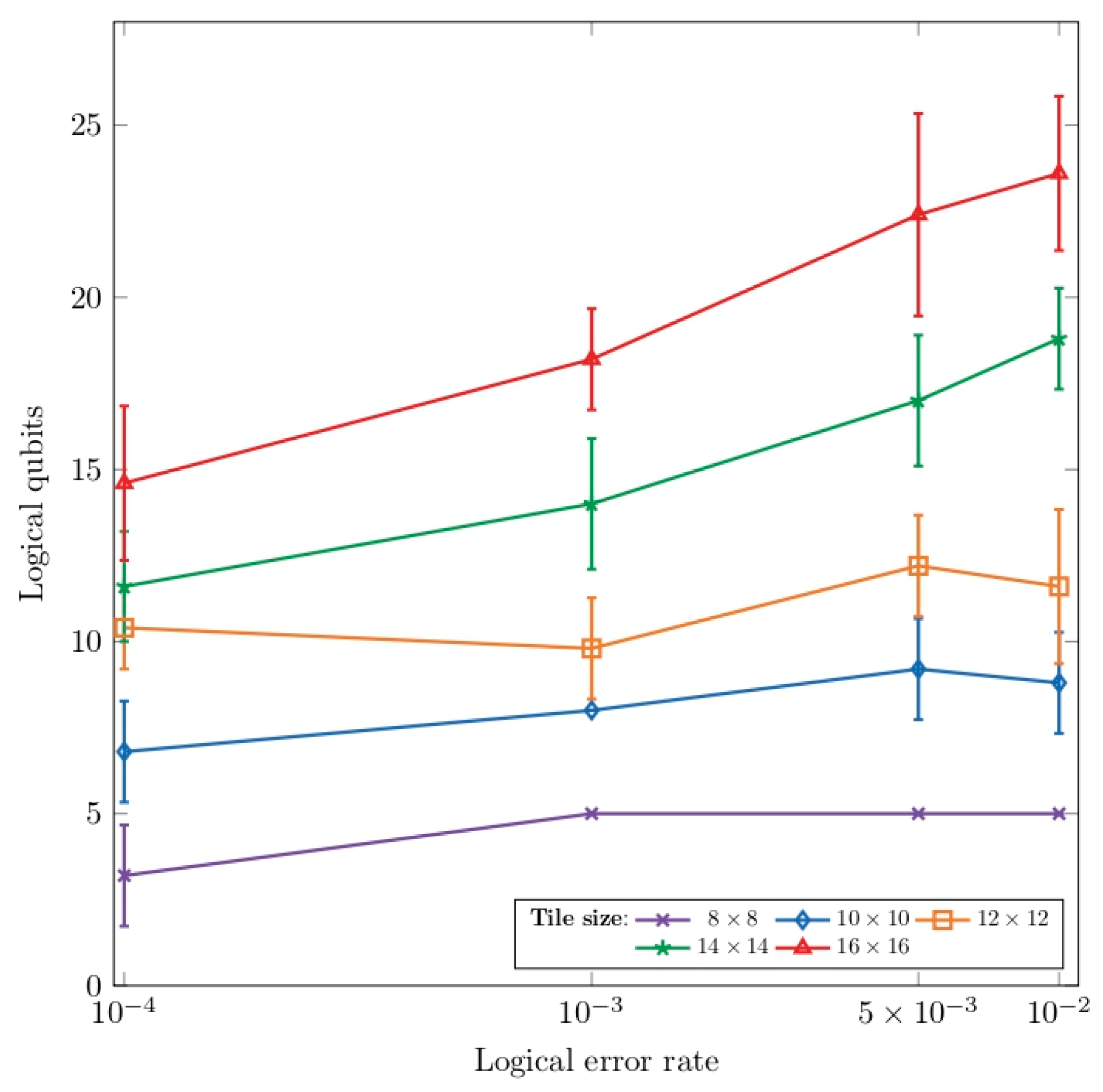As demonstrated in Section 2.6, partially open holes can encode more logical qubits in a square lattice. Therefore, we anticipate that square lattices with partially open holes can encode more logical qubits compared to lattices containing closed holes of similar code distance values. We set the code distance to 3 and assess the maximum number of qubits for a specific range of logical errors, just like in the prior section. To be more concise, in this part of the experiments, we only utilize the simulated annealing approach, with an initial temperature of 2400 K, and employ 1000 iterations. Similar to the previous analysis, we also examine how the approach behaves across different sizes of square lattices.

Figure 9 depicts the results of using partially open holes to encode logical qubits, showing that, on average, it leads to two to three times as many logical qubits as closed holes. These findings align with Equation (7) and demonstrate that surface codes with partially open holes yield more logical qubits under the same logical error rate. As in the previous case, the code distance acts as a limiting factor in increasing the number of encoded logical qubits. Additionally, we should consider the impact of partially open holes on errors by comparing the average number of placed closed and partially open holes.

Table 1. Number of holes and logical qubits for different logical error thresholds in $14\times 14$ square lattice.

Logical Error	Closed Holes		Partially Open Holes
	Logical Qubits	Number of Holes	Logical Qubits	Number of Holes
${10}^{-4}$	4.20	3.20	12.20	4.40
${10}^{-3}$	5.40	4.40	12.20	4.40
$5\times {10}^{-3}$	9.60	8.60	16.40	5.80
${10}^{-2}$	11.40	10.40	18.40	6.60

shows the average number of holes and logical qubits for different logical thresholds in a 14 × 14 square lattice obtained by SA. We can see that SA, on average, places more closed holes in a lattice than partial open holes under the given logical error. The results suggest that partially open holes increase the logical error rate, thus aligning with our expectations. Removal of the stabilizer (represented by faces) and additional adjacent physical qubits (partially open edge) lead to worse error behavior than only removing the stabilizer (closed edge). However, partially open holes form more logical qubits in square lattices than closed ones.

4.3. Influence of Parameters of Optimization Algorithm on Numbers of Logical Qubits

In previous experiments, we employed the SA and GA to assess the number of logical qubits which can be encoded by inserting defects in 2D lattice. However, we only assess the performance of optimization for fixed value of hyperparameters. The performance of simulated annealing (SA) and genetic algorithms (GAs) is sensitive to hyperparameters that influence convergence, exploration–exploitation balance, and solution quality. In SA, factors like maximal temperature and cooling schedule affect the size of solution space; slower cooling enhances global search but increases computation time, while faster cooling risks premature convergence. In GAs, parameters such as population size, crossover probability, and mutation rate manage genetic diversity and the ability to escape local optima. Effective tuning of these parameters is essential for robust optimization, often requiring problem-specific experimentation and heuristics.

To evaluate the influence of hyperparameters on algorithm performance, we assessed the number of logical qubits produced by SA and GA under varying hyperparameter settings. Our analysis focused specifically on a lattice $16\times 16$, targeting a logical error rate of $5\times {10}^{-3}$ to ensure an adequately large solution space. For SA, we investigated the impact of the maximum temperature (T_MAX) and the number of cooling steps. By selecting higher maximal temperatures and increasing the number of annealing steps, we aimed to investigate whether the SA algorithm could effectively explore the solution space to find lattices that encode a greater number of logical qubits. Regarding the GA, our analysis examined the effects of the number of generations and the number of parent solutions. The obtained results are summarized in

Table 2. Influence of SA hyperparameters on the number of obtained logical qubits in a 2D lattice.

TMAX	2400 K	4800 K	7200 K
No. of Steps
500	8.80 ± 0.75	8.20 ± 0.75	8.20 ± 1.17
1000	9.40 ± 0.49	9.20 ± 0.40	9.00 ± 0.63

and

Table 3. Influence of GA hyperparameters on the number of obtained logical qubits in a 2D lattice.

No. of Solutions per Generation	50	200	400
No. of Generations
500	9.80 ± 0.75	9.60 ± 0.80	9.40 ± 0.49
1000	9.80 ± 0.40	10.00 ± 0.63	10.00 ± 0.63

.

The results presented in Table 2 indicate that the maximum temperature parameter of the SA algorithm has a negligible effect on the obtained number of logical qubits. In contrast, increasing the number of annealing steps results in marginal improvement, yielding less than one additional logical qubit on average. This limited gain can be attributed to the intrinsic constraints of surface codes: for a given threshold, the code reaches a point beyond which additional holes in the code significantly degrade the error behavior. These conclusions are further supported by the data in Table 3, as they exhibit similar trends. Specifically, the number of logical qubits produced across different configurations of the GA remains comparable, with variations falling within the range of standard deviation. Although GA yields a higher number of encoded logical qubits compared to the SA approach, the final counts remain relatively close.

In addition to the previously conducted experiments, we further analyzed the influence of SA hyperparameters on the number of logical qubits generated by inserting holes with partially open edges into the lattice. Introducing partially open edges significantly enlarges the solution search space, compared to scenarios involving fully closed-border edges, due to increased degrees of freedom for hole placement and shape optimization. As in previous experiments, we investigated the impact of maximum temperature and cooling steps.

The results presented in

Table 4. Influence of SA hyperparameters on the number of obtained logical qubits with partially opened holes in a 2D lattice.

TMAX	2400 K	4800 K	7200 K
No. of Steps
500	20.00 ± 1.90	18.80 ± 3.06	20.60 ± 1.20
1000	23.60 ± 1.20	21.80 ± 1.47	21.20 ± 2.40

demonstrate a greater sensitivity of the simulated annealing (SA) algorithm to its parameter settings, which can be attributed to the larger search space in this instance. However, the observed variations in the number of encoded logical qubits remain within the bounds of the mean and standard deviation. These findings further highlight the limitations of surface codes, suggesting that their capacity to encode logical qubits is fundamentally restricted.

4.4. Influence of Code Distance on Error Characteristics

In the previous section, we analyzed the maximal number of qubits for a specific logical error rate. However, this analysis was specifically focused on a code distance of three. To understand how the code distance affects the error behavior of the surface code, we utilized optimization algorithms in a different scenario. Instead of aiming to find the maximum number of logical qubits for a given logical error rate, our focus shifted to holding the number of logical qubits at one and attempting to identify a surface code with a minimal logical error rate. In other words, our goal is to minimize the logical error rate while keeping the number of logical qubits fixed at one in the surface code. We employ only closed holes because we do not consider the number of logical qubits.

In our optimization algorithm, the code distance serves as a parameter. Like in the first experiment, the SA process is initiated with an open boundary square lattice. When adding a new hole, the hole needed to have d bordering edges and be at least $d-1$ faces away from the lattice border for a code distance of d. A larger code distance could result in a reduction in the number of holes placed on the lattice. Therefore, we only considered codes with two logical qubits or one hole in the lattice with an open border for each code distance. To generate potential solutions for SA, we added a hole whose size was determined by the code distance and moved it across the lattice.

To evaluate potential solutions, we employ hyperbolic tangents for energy function:

$$E=\tanh (LER)$$

(16)

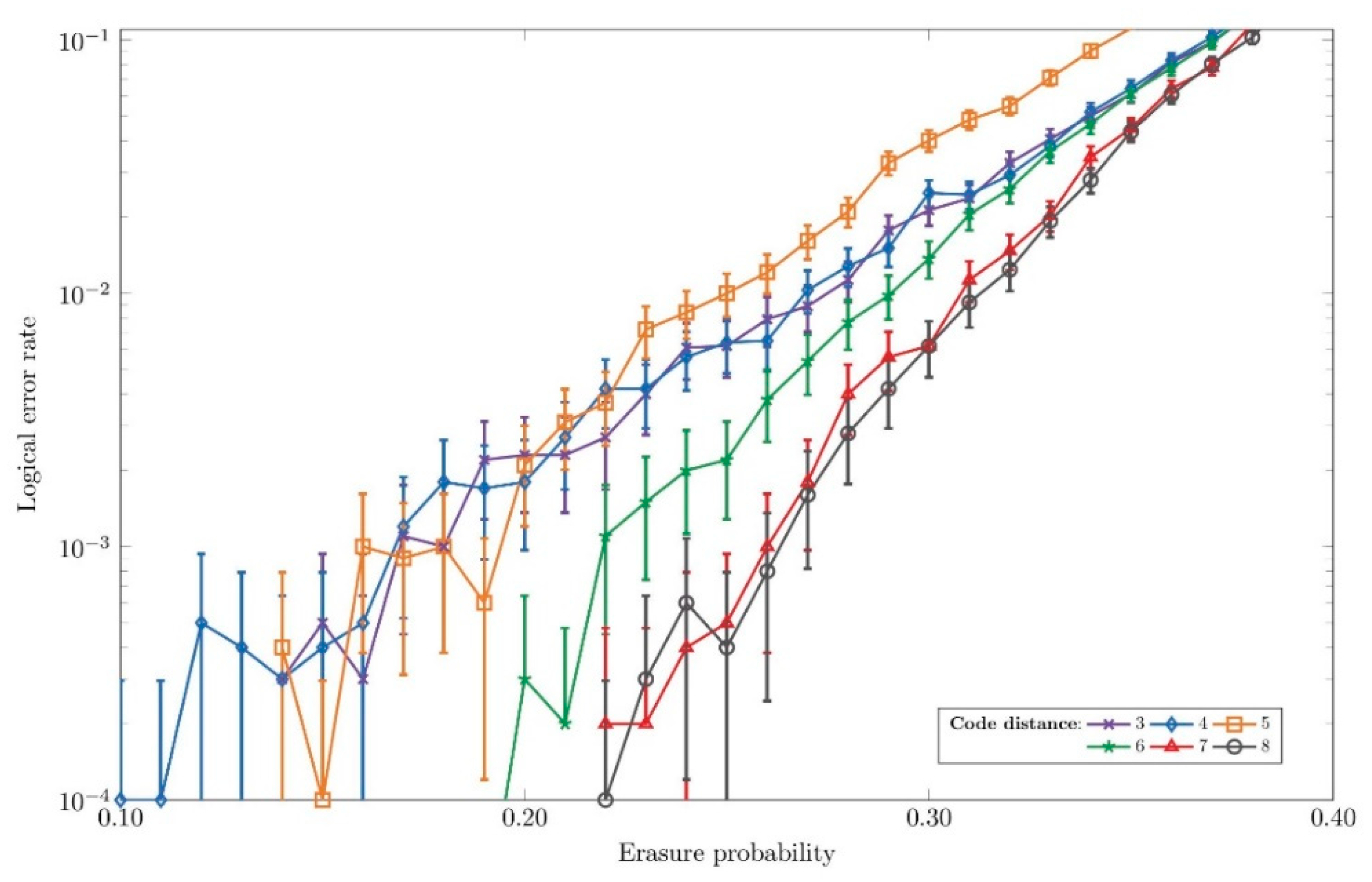
where LER represents the logical error rate obtained for the current solution in this equation. The energy function saturates large values of error rate, thus pushing the SA algorithm to avoid a hole position with a large logical error rate. Figure 10 illustrates the error characteristics of the obtained $18\times 18$ surface codes with varying code distances on a lattice encoding two logical qubits. From the image we can differ three groups of that share similar error performance. The tiles with code distances of 3, 4, and 5 exhibit the poorest error performance. In contrast, tiles characterized by code distances 7 and 8 demonstrate the best performance, achieving the lowest logical error rates across the evaluated erasure probabilities. Between these two lies the error distribution corresponding to tiles with a code distance of 6. These results align well with the expected behavior of surface codes, where increased code distance results in improved error resilience. However, it is important to emphasize that, in a defect-based encoding approach, increasing the code distance involves strategically removing physical qubits (creating defects) rather than adding qubits to the lattice.

5. Discussion

The previous sections have demonstrated the potential of a defect-based approach for encoding multiple logical qubits. These results are based on the Squab simulator, which evaluates the error rate of examined lattices. While practical implementation aspects of defect-based encoding are beyond the scope of this paper, this section reflects on our findings to highlight specific advantages and limitations inherent to this approach and analysis.

We first consider the encoding density achieved by our method. Referring to the results obtained for different logical error thresholds on a 14×14 square lattice (Table 1), the lattice configuration consists of 420 physical qubits, yielding a maximal encoding density of up to 30 physical qubits per logical qubit. To evaluate the effectiveness of our approach, we compare our results with the theoretical limitations for logical qubit packing in planar surface code. According to Delfosse et al. [8], the maximum number of logical qubits encoded via closed holes is approximately as follows:

$$\mathrm{n}\sim 3{\mathrm{kd}}^2$$

(17)

where n denotes the number of physical qubits, k is the number of logical qubits, and d is the code distance. For a 14 × 14 lattice with a code distance of 3, the theoretical maximum equals 15 logical qubits. As indicated in Table 1, our SA algorithm achieves results very close to this theoretical limit. However, it is important to emphasize that Delfosse et al. [8] do not consider logical error rates when deriving their theoretical bounds for logical qubit encoding on square lattices. Moreover, our results for lattices incorporating partially open holes are aligned with the conclusion presented in [8], demonstrating that partially open defects offer distinct advantages over standard surface codes for storing quantum information within two-dimensional lattices.

In the experiments, the simulator assumes that the decoding algorithm knows the locations of the erased qubits, which can usually be measured in experimental setups. Decoding stabilizer codes within this context entails solving a linear system, which generally has cubic complexity. However, real-life decoding is more complex than demonstrated in experimental settings. One significant downside of the defect-based approach is the complexity involved in decoding stabilizer measurements. The author in [39] employs a tensor-network decoding algorithm for near-optimal error correction. The approach revolves around modeling logical channels. According to the proposed approach, the complexity of encoding is related to a logical channel, with its size increasing exponentially as the number of encoded logical qubits rises. Nevertheless, they do not dismiss the possibility of an optimal decoder within this framework. Several machine learning-based decoding algorithms have recently been introduced to enhance performance and reduce latency in QEC codes [40]. Given their rapid and constant inference time and State-of-the-Art decoding performance, we anticipate that neural network-based decoding will provide an effective solution for correcting errors in surface codes containing holes.

While our simulation results demonstrate the potential advantages of the defect-based approach, we must acknowledge limitations in our benchmarking methodology. The erasure channel model employed by Squab assumes perfect knowledge of erasure locations, representing an idealization of real quantum hardware. In physical implementations, detecting erasures would require additional measurement circuitry and syndrome extraction rounds. These measurements could introduce errors by themselves, and pausing the main syndrome extraction to check for erasures could allow other errors to accumulate. Additionally, real detection mechanisms might suffer from false positives (incorrectly identifying intact qubits as erased) or false negatives (failing to detect actual erasures), thus affecting the decoder’s performance. Though these practical considerations are not captured in our current simulations, they represent important engineering challenges for implementing defect-based surface codes in hardware. The theoretical performance bounds established in this work provide targets for hardware implementations to aspire to, while acknowledging that practical implementations will likely operate with some performance gap relative to these idealized results due to the overhead of erasure detection.

In physical implementations of surface codes, erasure detection requires specific measurement protocols. In superconducting qubit platforms, erasures often manifest as leakage events where the qubit state leaves the computational subspace. These leakage events are detectable through high-fidelity readout schemes that can discriminate between computational states and leakage levels. The detection typically involves applying controlled operations between the potentially leaked qubit and an ancilla qubit, followed by measurement of the ancilla [41,42,43]. For trapped ion systems, erasures might correspond to ion loss or transitions to unwanted electronic states, which can be detected through fluorescence measurements [44,45]. The physical noise sources that generate erasures include microwave pulse miscalibration in superconducting circuits, laser intensity fluctuations in trapped ions, and environmental coupling effects. Experimental implementations often use engineered noise channels to benchmark code performance, where controlled perturbations are deliberately introduced through miscalibrated gates or engineered coupling to simulate realistic error processes [43,45].

6. Conclusions

Expanding the number of logical qubits is crucial for advancing quantum computing, especially in the NISQ era. While the patch-based approach for encoding multiple qubits is prevalent, it is equally important to explore the potential of the defect-based approach. The latter method, which encodes logical qubits by placing the holes in a lattice, poses a trade-off between the number of logical qubits and logical error rates. To tackle the trade-off above, we employed optimization algorithms, including SA and GA, to assess the maximum number of logical qubits for a given error rate. As expected, larger lattices yield a larger degree of freedom when moving the holes in code, and, thus, we can accommodate more logical qubits for a range of error rates. The results also revealed properties of partially open holes, which help encode more logical qubits than closed holes, showcasing the potential for improving the code density behind defect-free approaches. We also conducted experiments regarding code distance and holes in surface code. The findings show that higher code distances result in better performance for error correction. While existing research, such as the development of patch-based quantum processors like Google’s Willow [46], favors a patch-based approach for encoding multiple qubits, combining patch-based and defect-based approaches could lead to more efficient encoding of logical qubits. For instance, defect-based methods may offer higher qubit density or improved scalability when integrated with patch-based architectures. Exploring the synergy between these approaches is an area we plan to investigate further in our future work.

In addition, while defect-based surface codes support braiding-based logical operations without ancillary patches, preserving the effective code distance during such dynamic operations remains a critical challenge. Improper spacing or routing of defects during braiding may reduce the minimum distance, increasing the risk of logical errors. Future work will extend our current framework to explore strategies and automated techniques for preserving code distance during braiding, potentially by integrating braid scheduling heuristics or adaptive layout constraints into the optimization process.

Finally, we acknowledge the limitations of our current benchmarking approach. Our simulations rely on the erasure channel with perfect knowledge of erasure locations; it provides computational efficiency but idealizes certain aspects of physical implementations. In practice, detecting erasures would introduce additional complexity, potential errors, and overhead not captured in our current model. Future work should expand our analysis to include more realistic noise models that account for imperfect erasure detection, false positives/negatives in detection mechanisms, and the additional error sources associated with erasure checking in physical implementations. Combining more comprehensive noise models with our optimization approach would provide even more robust guidance for practical implementations of defect-based surface codes in future quantum computing hardware.