Abstract
Modeling many-body quantum systems is widely regarded as one of the most promising applications for near-term noisy quantum computers. However, in the near term, system size limitation will remain a severe barrier for applications in materials science or strongly correlated systems. A promising avenue of research is to combine many-body physics with machine learning for the classification of distinct phases. We present a workflow that synergizes quantum computing, many-body theory, and quantum machine learning (QML) for studying strongly correlated systems. In particular, it can capture a putative quantum phase transition of the stereotypical strongly correlated system, the Hubbard model. Following the recent proposal of the hybrid quantum-classical algorithm for the two-site dynamical mean-field theory (DMFT), we present a modification that allows the self-consistent solution of the single bath site DMFT. The modified algorithm can be generalized for multiple bath sites. This approach is used to generate a database of zero-temperature wavefunctions of the Hubbard model within the DMFT approximation. We then use a QML algorithm to distinguish between the metallic phase and the Mott insulator phase to capture the metal-to-Mott insulator phase transition. We train a recently proposed quantum convolutional neural network (QCNN) and then utilize the QCNN as a quantum classifier to capture the phase transition region. This work provides a recipe for application to other phase transitions in strongly correlated systems and represents an exciting application of small-scale quantum devices realizable with near-term technology.
1. Introduction
Strong electronic interactions in quantum materials give rise to many phenomena that potentially harbor properties suitable for technological applications. Some notable effects include the metal-insulator transition, heavy fermions, frustrated magnetism, and non-Fermi liquid metals [1,2,3]. However, delving into the realm of strongly correlated systems poses significant challenges, primarily due to the absence of a suitable starting point for perturbative methods. This challenge is exemplified by our incomplete understanding of superconductivity in cuprates, despite decades of research [4,5]. Classical numerical methods have been employed to solve simplified models of strongly correlated systems, among various other important models, such as the Hubbard model [6,7]. However, these numerical methods are often hindered by the minus sign problem for Quantum Monte Carlo (QMC), or by the exponential growth of the Hilbert space with the system sizes for exact diagonalization. This prevents simulations from reaching low temperatures.
Amid these challenges, embedding schemes like dynamical mean field theory (DMFT) [8,9,10,11,12,13] have emerged as suitable alternatives, simplifying the many-body problem by approximating the complex lattice system as simpler impurity problem. Although this method solves problems in the higher dimensional limit, it yields many interesting results that are comparable to experimental observations. Notably, it captures the metal-insulator transition without any biased approximation [9]. The DMFT mapping is exact in infinite spatial dimensions, but is approximate for finite dimensions. The approximation can be improved by systematically incorporating corrections from the spatial dependence of the model. There are two main methods for including spatial correlations: perturbative approaches [14,15,16,17,18,19] and impurity cluster methods using multiple impurities [20,21,22].
Meanwhile, recent advancements in numerical algorithms and computing power have enabled accurate numerical solutions to the single-impurity problem. In particular, methods such as Dynamic Cluster Approximation (DCA) [20,21] and Cellular DMFT (CDMFT) [22] can tackle problems involving multiple impurity sites, although this comes at the cost of increased computational complexity, which still represents a significant bottleneck for the advancement of numerical studies in this field. Methods which further simplify DMFT have also been proposed to make the calculation more tractable. In particular, density matrix embedding theory (DMET) has seen successful applications in quantum chemistry [23].
Classical computing approaches for accurate solutions of strongly correlated systems face challenges due to exponential scaling, either in computing time (as in the minus sign problem in QMC) or storage (e.g., for exact diagonalization). This limitation hinders prediction for large systems and is unlikely to be overcome by classical hardware or algorithms. In recent years, a novel approach grounded in data science and machine learning has emerged to tackle the single-impurity problem [24,25,26,27,28]. Although this approach may provide an improvement in efficiency, the training process still relies on solutions from classical computing.
The emergence of quantum computing offers a new avenue. DMFT, for instance, can be tackled through a hybrid quantum–classical scheme [29,30,31,32,33], where quantum hardware solves the effective impurity problem while a classical computer post-processes the results. Although direct simulations of models with explicit electron–electron interaction, such as the Hubbard model, near the thermodynamic limit remain beyond current quantum computing capabilities, DMFT simulations on noisy intermediate-scale quantum (NISQ) devices are feasible as the impurity problem can be approximated with a few lattice sites. Nevertheless, computing excited states or Green’s functions remains a challenge for quantum computers in the quantum–classical hybrid scheme [34].
Utilizing quantum computing to solve DMFT poses a unique challenge due to the limited number of available sites or qubits, especially concerning the calculation of the excited state. In the infinite dimension limit, the excitation spectrum becomes a continuous function of energy. But with the constrained Hilbert space dimension, it is represented by discrete delta functions, necessitating a smoothing process for the calculations. This issue becomes particularly significant when extracting physical quantities around the Fermi level.
The integration of many-body physics and ML has shown promise in various studies, with classical ML traditionally employed for phase transition detection [30,32,33,35,36,37]. Quantum machine learning (QML) has emerged as a new paradigm, allowing the representation of input in terms of wavefunctions, fostering the study of phase transitions in many-body systems [37,38,39,40,41,42,43,44,45,46,47,48,49,50,51,52,53,54,55]. Quantum circuits as classifiers, inspired by classical neural networks, have been explored, particularly utilizing convolutional neural networks (CNNs) to identify different phases of matter and their transitions by extracting features from correlation functions of complex systems [52,56,57,58,59,60,61,62,63,64,65,66,67,68,69,70,71,72,73,74].
CNNs [75,76,77,78,79,80,81,82] have found extensive utility in physics, enabling pattern recognition in statistical models and the analysis of strongly correlated systems [36,83]. By incorporating convolutional layers into quantum neural networks, analogous to CNNs, spatial information among qubits can be analyzed effectively, showcasing potential in quantum computing for classifying phases and studying phase transitions [84,85].
Quantum-enhanced ML holds great promise for distinguishing different phases of matter shown by recent research [86,87]. The QCNN method might become feasible to recognize various phases of a quantum many-body system, a significant step toward detecting quantum phase transitions. To apply the QCNN approach, the input needs to be naturally quantum mechanical or generated from some filters that transform the classical data. This eliminates the representation of the wavefunction as a classical vector which grows exponentially with system size [88]. The required input should consist of a quantum circuit and the most effective approach for obtaining the wavefunction through the DMFT solution of the two-site single-impurity Anderson model (SIAM) is the variational quantum eigensolver (VQE) method executed on NISQ computers. The main goal of this study is to employ the QCNN to classify the VQE wavefunction obtained via the DMFT for the Hubbard model at the thermodynamic limit. This establishes a framework for detecting quantum phase transition in many-body quantum systems solved with the VQE method.
This paper presents a viable recipe for the study of strongly correlated systems, in particular the quantum phase transition in the thermodynamic limit with the NISQ. Specifically, we focus on drawing the phase diagram. The idea combines DMFT, VQE, and QML. The entire process can be implemented on NISQ computers except that the optimization of the parameters is performed by classical algorithms. The paper is organized as follows. In Section 2, we briefly describe the DMFT approach and its relation to the SIAM. In Section 3, the methods and procedure of the two-site DMFT are presented. The quantum simulation of the two-site Hubbard model is described in Section 4. The results for the impurity Green’s function, quasiparticle weight, and entanglement entropy are presented in Section 5. In Section 6, we use the wavefunction from the DMFT solution to train a QCNN for the detection of the metal-to-insulator phase transition. The results after training the QCNN for the classification of different phases are shown in Section 7. We conclude and propose possible future directions of using VQE and QML methods via DMFT for the study of strongly correlated systems.
2. Dynamical Mean Field Theory (DMFT)
Our starting point for strongly correlated electrons is the Hubbard model defined by the following Hamiltonian:
where the electrons hop between adjacent lattice sites i and j, denoted by , with amplitude . Without specification, we set , and its also serves as the energy scale. The inverse of t serves as the time scale. and respectively denote the creation and annihilation operators for an electron of spin at site i. is the number of particles with spin at the site j. The interaction between electrons is governed by the on-site Coulomb repulsion of strength U.
The outline of DMFT is shown in Figure 1. The key step of the DMFT algorithm is to find the Green’s function of the effective impurity model. There are two major types of methods to address this challenge, QMC methods based on sampling the partition function directly or Hamiltonian methods based on the discretization of the electron bath into a finite number of so-called bath sites.
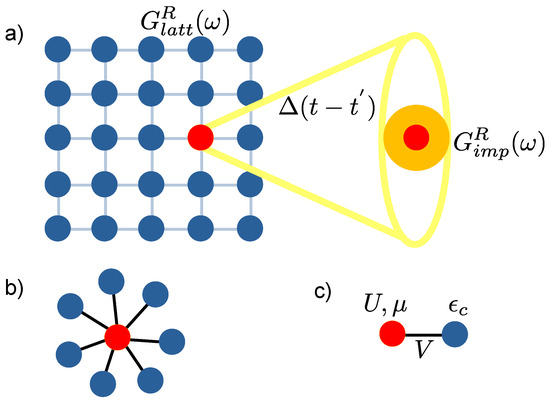
Figure 1.
(a) Dynamical mean-field theory (DMFT) neglects spatial fluctuations, the lattice model with local interaction is mapped into a single site problem and the rest of the lattice is replaced with an effective frequency-dependent mean-field subject to the self-consistency condition. (b) The non-interacting bath sites are connected to the central, interacting impurity site. (c) Minimal representation of the two-site DMFT, where V is the hopping strength between the impurity site (red dot) and the bath site (blue dot).
The minimal model to mimic the impurity problem is the two-site representation proposed by Potthoff [89] (shown in Figure 1c),where hopping occurs only between sites 1 and 2, defined as V in Equation (A10). The value of V is determined by the DMFT self-consistent equation, the detail can be found in the Appendix A.
It consists of one site representing the impurity and only one site approximately representing the bath. We refer the reader to Appendix A.1 for the detailed steps of the DMFT algorithm and Appendix A.2 for the two-site DMFT.
3. Methods and Procedure
After the formulation of the two-site DMFT, the next step is to transform the problem from fermionic operators into spin- operators for the quantum algorithms. The ground state of the Hamiltonian is obtained by the variational quantum eigensolver (VQE) and Green’s functions are then calculated via the Trotter–Suzuki approximation. With Green’s function, the quasiparticle weight can be calculated and the self-consistency equations can be solved. The procedure is repeated until the desired convergence of the quasiparticle weight is attained. We only consider the half-filled case in this study, so that the chemical potential can be fixed by hand exactly by explicitly enforcing the particle–hole symmetry. The procedure largely follows that of Kreula et al. [31] and modified by Keen et al. [30]. We outline their algorithms here and highlight the differences we propose for calculating the quasiparticle weight.
3.1. Jordan–Wigner Transformation for Mapping the Fermions to Qubits
We follow the standard Jordan–Wigner transformation to transform the fermionic creation and annihilation operators into spin operators for representation on a quantum computer. A four-qubit system (excluding the ancilla qubit which is used for measurement) is required to represent the two-site SIAM. The spin-down information is encoded by the first two qubits for sites one and two, while the corresponding information for the spin-up occupation is encoded by the third and fourth qubits. The use of Jordan–Wigner transformation to represent Green’s function for the two-site model first appeared in Kreula et al. [31] and later in Keen et al. [30]. The detailed explanation of the mapping can be found in Appendix A.3.
Following the calculation in Appendix A.3, the retarded impurity Green’s function can be measured. As the functional form of the two-site problem is known, one can fit the function on a classical computer. For the two-site DMFT, the interacting Green’s function is a four-pole function due to the presence of particle–hole symmetry,
where at half filling. Fourier transforming the above equation leads to
where is an artificial broadening parameter. Once the self-consistency is attained, the Dyson equation is used to calculate the self-energy and, subsequently, the spectral function is obtained by .
3.2. Self-Energy of the Two-Site Model
A common practice for calculating the self-energy is to employ the Dyson equation in the frequency domain [9]. Since is given as the input of the impurity problem and is obtained by the above fitting procedure via Fourier transform. The self-energy can be seemingly easy to obtain by
where the bare Green’s function is
Since the quasiparticle weight is given by the derivative of the real part of the self-energy at zero frequency, we need to solve the Equation (A16) at zero frequency. Unfortunately, it is not easy to calculate the self-energy accurately, as the number of states in the two-site system is very limited, the subtraction of the two Green’s functions in the Dyson equation is essentially a subtraction of a set of delta functions. This does not pose a serious issue when the bath is in the continuum and it is performed routinely in most numerical DMFT calculations [9]. However, the limited number of states available in the present problem makes the results highly sensitive to the choice of the damping parameter in the Fourier transform of Green’s function from the real-time domain to the frequency domain. Strictly speaking, there is also a damping factor associated with time, however, the available time in the present calculation is always limited to a finite value.
Keen et al. [30] proposed a remedy for this issue. The idea is, instead of calculating the self-energy at zero energy by subtracting the inverse of the bath and the interacting Green’s function at zero, to consider the sum over a window of energy. This provides more stable and consistent results, less dependent on the damping factors [30].
This is a effective method for achieving better stability in the iteration step of finding the self-consistent solution of the DMFT. As far as the two-site DMFT is concerned, this integration method is applicable. However, for more general settings such as the cases for multiple bath sites, the self-consistency is more involved. Instead of just the quasiparticle weight, the full self-energy needs to be obtained and the integration method cannot be readily generalized for those situations. Moreover, the integration method also brings an additional parameter that cannot be fixed simply. Therefore, it is desirable to have a method that has minimal dependence on arbitrary parameters, specifically the damping and the integration range, but is sufficiently stable for the iterative solution of the DMFT equations. We observe that the system is a finite-size cluster, therefore the self-energy of the two-site impurity problem is a two-pole function of the form [89],
The self-energy is completely determined by five parameters, , , , and , where and at half filling. Once we have its explicit form, we can Fourier transform the self-energy back to the time domain with the explicit form of it. The functional form will be the same as that of Green’s function. Instead of calculating the self-energy in the frequency domain, we can also use the Dyson equation in the time domain to compute the self-energy. Both the inverse of the bath and interacting Green’s function are well behaved. The parameters, , , and are then obtained by fitting the self-energy as the difference between the inverse of the bath and the interacting Green’s functions in the time domain. After performing the fitting procedure, the full self-energy is obtained and can be used to extract quasiparticle weight and any other physical quantities.
The self-energy obtained in this way has a minimal number of arbitrary parameters. The remaining arbitrary parameters are the upper limit of the time and the time step in the Trotter–Suzuki approximation, which are both intrinsic limitations of the quantum algorithm. Therefore, no additional arbitrary parameter is introduced except those limited by the quantum algorithm.
3.3. Flowchart of the Algorithm
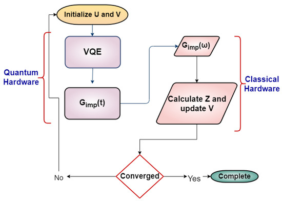
Figure 2.
The two-site DMFT calculation flowchart implemented on a hybrid quantum–classical system.
- U and are fixed to the desired value in the SIAM, and we set the unknown parameters for half-filling, and V to an initial guess.
- Then, we measure the interacting Green’s function using the technique of single-qubit interferometry.
- We Fourier transform the impurity Green’s function by fitting it according to Equation (2).
- We calculate the coefficients for the self-energy by using the Dyson equation in the time domain.
- We measure the quasiparticle weight using the self-energy.
- We update the hopping parameter V.
- We repeat steps 2–6 until the self-energy is converged.
The algorithm was first proposed by Kreula et al. [31] and modified by Keen et al. [30] for the calculation of the quasiparticle weight. For the half-filled case, the only external parameter is the Hubbard U. The iteration for the self-consistent solution for the quasiparticle weight starts from a given U and an initial guess for V. With these values of U and V, the two-site impurity problem is solved by finding the ground state by the variational quantum eigensolver(VQE) and then Green’s function in real-time is obtained by propagating the ground state using the evolution operator . The above procedure can be performed in quantum hardware except for the minimization process for the VQE. Once Green’s function in real time, , is obtained, we find the Fourier transformed Green’s function by a fitting procedure as explained in Section 3.1. With the , the quasiparticle weight, , can be calculated by using Equation (A17). With the obtained , we can update the hybridization V, using the relation . Then, the V is checked for convergence. The fitting process is performed in the classical hardware.
4. Implementation
4.1. Ground-State Ansatz
The variational ansatz is a quantum circuit with eight single qubit rotations, and three CNOT gates, see Figure 3. The VQE then optimizes the single qubit rotation parameters to minimize the expectation value of the target Hamiltonian for given values of to obtain the ground state of the system. It is important to understand that there is not a unique way to choose a variational state. Selecting the optimized variational ansatz is an important but unsolved problem, both in classical variational methods like Variational Monte Carlo (VMC) and in our work. In this study, we are not trying to discover the ’best’ wavefunction [30,31].
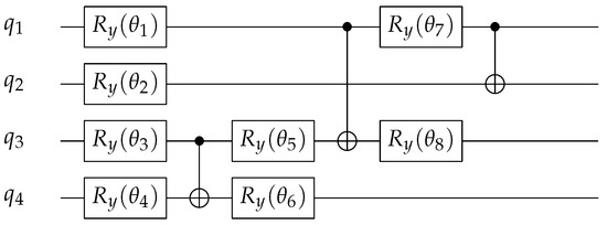
Figure 3.
Quantum circuit for the ground-state ansatz. We use the same wavefunction for the VQE as in Kreula et al. [31] and Keen et al. [30].
The ‘best’ wavefunction varies with the model and the parameters involved [90]. Here, we keep the same functional form of the wavefunction across the entire range of on-site interaction strength, even though it may not be the ‘best’ optimized wavefunction.
4.2. Retarded Impurity Green’s Function
The measurement of the impurity Green’s function is performed by a single-qubit Ramsey interferometer, shown in Figure 4 [31,91]. An ancilla qubit is introduced in addition to the ‘system’ qubits; therefore, five qubits are needed to implement the two-site DMFT.
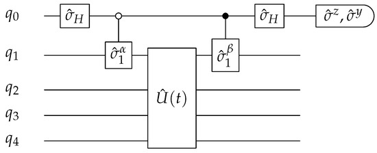
Figure 4.
Quantum circuit for measuring the individual components of . is composed of quantum gates. is the Hadamard gate. and can be and according to the components in Equations (A26) and (A27) that we measure. The white (or black) dot represents a controlled gate operation on qubit depending on qubit is in (or ) state.
5. Results
We obtained the results using a simulator running on classical computers. We start by examining the procedure of obtaining the impurity Green’s function in the DMFT routine. Figure 5 shows the impurity Green’s function for (top) and (bottom) with , respectively. We superimpose the data in Figure 5 to the fit obtained according to the exact result of Equation (2). The calculated Green’s function data are obtained with a modest number of time steps (18 in this case).
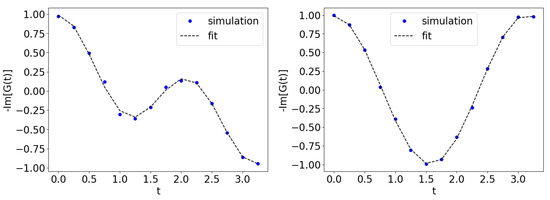
Figure 5.
(Left) Impurity Green’s function for and . The parameters for the fit shown are , , , . (Right) Impurity Green’s function for and . The parameters for the fit shown are , , , and . We fit the impurity Green’s function to Equation (2).
The impurity Green’s function in the frequency domain is extracted from the fit parameters following Equation (3). We obtain the energies and from fitting the Green’s function to Equation (2) for half-filling. We then Fourier transform the impurity Green’s Function according to Equation (3) to the frequency domain. We use the Dyson equation to calculate the self-energy in the frequency domain from Equation (A16). We obtain the parameters , and , by fitting the self-energy to Equation (6). Figure 6 shows the quasiparticle weight at self-consistency using Equation (A17) for U values ranging from to .
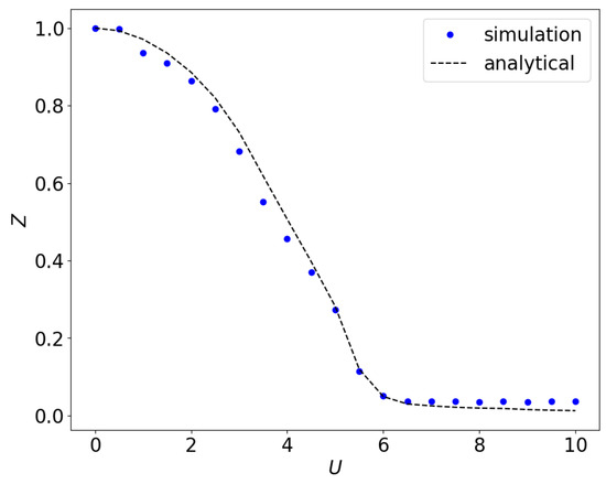
For and half-filling case, the self-energy of the two-site SIAM can be calculated analytically [89]:
With Equation (A17), this gives the quasi-particle weight:
In addition to the quasiparticle weight, another quantity that may indicate a phase transition is the entanglement entropy. It has been tested extensively on fermionic lattice models that entanglement, combined with finite size scaling, can be used to determine the critical point [92,93,94]. The idea of using entanglement entropy within DMFT has not previously been explored in detail. There is a clear choice of dividing the system into two parts here, as the effective problem that is being solved in DMFT is the SIAM. We can define the entanglement entropy between the impurity site and the bath sites naturally, that is,
where is the reduced density matrix for the impurity site. It is obtained by tracing out the degree of freedom from the bath sites in the density matrix for the ground state (). That is , where . We refer the reader to Appendix A.4 for details of the entanglement entropy calculation. As already mentioned, the VQE optimizes the parameters of the quantum circuit shown in Figure 3 to minimize the expectation value of the target Hamiltonian for given values of to obtain the ground state of the system. The behavior of the local entanglement for the half-filling case is shown in Figure 7.
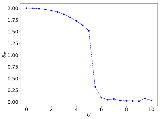
Figure 7.
Local entanglement of the two-site SIAM at half-filling versus the on-site coupling U calculated using Equation (9).
6. Classification Using Quantum Machine Learning(QML)
In the large U limit, , all sites are singly occupied, and one gets . For finite U, the hopping process enhances , and hence reaches its maximum value, 2 at . There is a sharp change near the value of U corresponding to the Mott transition as estimated from the quasiparticle weight.
In the previous section, we obtain Green’s function of the Hubbard model under the DMFT approximation. In addition, we also have the wavefunction for the effective impurity problem from the DMFT. Instead of directly calculating an ’order parameter’, we try to identify the different phases from the wavefunction. It is worthwhile to note that, unlike the DMFT with a continuum bath, the system here is a finite-size system, therefore, there is no true phase transition as that of the thermodynamic limit. Notwithstanding this noteworthy deficit, it has been shown that classical ML methods can locate phase transitions as well as crossovers rather accurately from finite-size classical and even quantum systems [37,44].
6.1. QML as a Classifier of Wavefunctions
Since our data are inherently quantum, it is natural to involve a QML approach to try to identify the phase transition. In the present study, we focus only on supervised learning. Exactly as in classical ML, the first step is to label input objects [44]. The input object here is the wavefunction, and the label is whether the wavefunction corresponds to a metal or insulator.
The major conceptual difference between the QML and the classical ML approaches is in the input data and the function that generates the output label. A popular choice for classical ML is to treat the input data as an array of numbers, and the function is usually chosen as a form of neural network. For supervised learning, a data set consists of input objects, and their corresponding labels are then used to optimize the parameters in the neural network during the training.
Most applications of QML are focused on using classical datasets [95]. We usually convert the wavefunction represented as a classical vector into quantum data. This is the exact process that a quantum classifier requires for classical data. For the present study, the input is wavefunctions from the converged DMFT solution, a genuinely quantum dataset, represented in quantum circuits from the VQE.
6.2. Implementation of the Quantum Convolutional Neural Network (QCNN) to Classify the Wavefunctions from the DMFT
Our objective is to showcase the effectiveness of the QCNN in identifying wavefunctions at different phases. From the converged DMFT solution, we obtain the input wavefunction, and the output label determines whether the wavefunction corresponds to a metal or an insulator.
The quantum neural network [95,96] is a direct conceptual generalization of the classical neural network; the main difference is that the activation functions [95,97,98] are replaced by quantum gates and the input and output are replaced by quantum states instead of an array of classical variables. The quantum neural network we employed in the present study is denoted as QCNN [85]. A QCNN consists of two distinct layer types: the pooling layer and the convolution layer. The number of degrees of freedom is reduced by the pooling layer and is substituted by multi-qubit gates, the CNOT gate being the simplest option [85]. The convolution layer in the classical CNN is substituted by multi-qubit quantum gates among adjacent qubits.
The QCNN is built by arranging convolutional and pooling layers in an alternating pattern until the number of pooling layers is reduced to just one qubit or the desired number of qubits. The goal of the present study is to use the QCNN to extract important information from the input quantum data and correctly identify the ’phase’ of each wavefunction. We can then use the results to predict the quantum critical point of the Hubbard model via the DMFT. We train the QCNN in a supervised environment, where the correct phase identification for each data point is already known. For a given on-site interaction U at the half-filling, the two-site DMFT approximation can give a metallic or Mott-insulator phase. The metallic phase is below and the Mott-insulator phase is above [89]. The reader may refer to the details of the QCNN circuit outlined by Cong et al. [85].
7. Classifier Results Using a QCNN
The QCNN was trained using two different selections of training data. 200 data points are generated for different U uniformly distributed over . In the first set of training, the QCNN randomly selects of the wavefunctions with labels to indicate their corresponding phases, forming the training data set. In the second set, the data points corresponding to low and high on-site interaction, U were used for training. The metallic phase was assigned the label , while the Mott insulating phase was assigned the label . The accuracy of the predictions was benchmarked by rounding the output to when the QCNN output measurement was smaller than 0 and to +1 when the measurement was greater than 0.
7.1. Training QCNN with Data for Randomly Picked Data for
We evaluate the performance of our trained QCNN by using the remaining of the samples as a benchmark and track the loss and accuracy at each iteration of the training process. We plot the loss and accuracy as a function of epoch in Figure 8. The accuracy is calculated by taking the mean of the tensor which is obtained after checking element-wise equality between the true labels and the predictions. It can be defined as
where is the true label of the sample, is the predicted label of the sample. The function is 1 if or 0 otherwise, and N is the total number of input samples. We find the loss from calculating the mean of squares of errors between the true labels and the predictions [95]. It is defined as
where y are the true labels, x are the input feature vectors, which are wavefunctions, and are the output predictions. N is the total number of input samples.
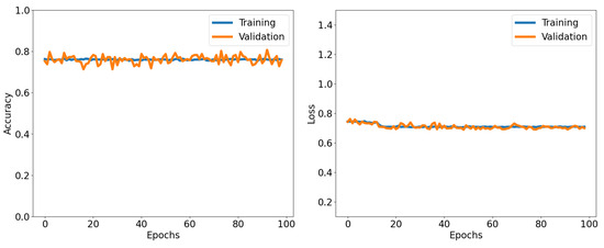
Figure 8.
Accuracy and loss as functions of the number of epochs for both the training and validation datasets in the QCNN. Training with randomly picked data for . Accuracy is the mean of the tensor calculated after checking element-wise equality between the true and predicted labels. Accuracy and loss are calculated using Equations (10) and (11).
By randomly selecting wavefunctions for training, QCNN is capable learn from the complete dataset, encompassing samples from both close and distant regions in relation to the quantum critical point for various U values. This allows the QCNN to become well versed in the wavefunctions and provide accurate predictions for the trained data. We achieve an accuracy of for both our training and testing datasets, with minimal fluctuations observed throughout the entire process. This demonstrates that randomized training data enables the QCNN to adapt to fluctuations in wavefunctions in the training and generalize well to testing data. The QCNN exhibits the ability to predict the phase of wavefunctions, and we observe the training process through the loss values of the network. Once the loss converges, indicating no further decrease, the QCNN is considered fully trained and operating at its peak efficiency. Despite the high loss values and insignificant convergence of the loss, each iteration demonstrates the system’s training progress. We can visualize the QCNN’s training phase and observe its improvement in predicting correctly the phase corresponding to the wavefunctions. In Figure 9 we plot the average value of the predicted label as a function of U. We average over 10 data points to find the average label, we find that the label passes through zero around .
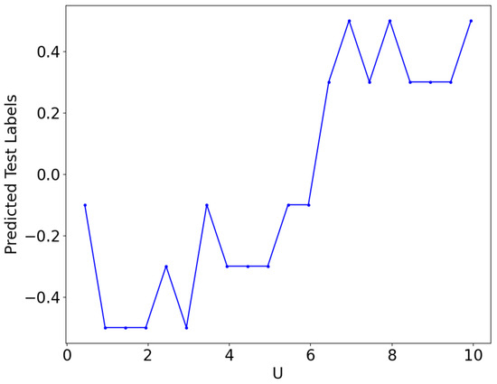
Figure 9.
Predicted test labels vs U. The predicted labels show a jump from a negative to a positive value around . Testing randomly picked data for .
7.2. Training QCNN with Data for and
After considering the aforementioned findings, we opted to assess the performance of the QCNN using selected training and testing data. During training, we used wavefunctions that had U values below and above , while the test data were within the range of [4.0–7.0]. This approach allowed us to determine how effectively the QCNN classifies data close to the known quantum critical point after training it with data away from it. During training, we obtained an accuracy rate of approximately 75–80%, which is not surprising given that the two sets of data with very large and very small values of U are quite different from each other.
We present the results in Figure 10 and Figure 11. We observed that the testing data consistently exhibited a lower accuracy rate than a randomized dataset. The QCNN is somewhat capable of classifying data points that are far from the quantum critical point. However, as the quantum phase transition approached, the predictions become difficult for the network. The average predicted label shows the crossing from negative to positive values for U between 5 and 6. The lack of familiarity with data points in this range limited the accuracy of the testing data. During the training phase, the loss had only slight changes compared with the use of randomized data, and while there was still a decrease, it was minimal. This suggests that the present implementation of the QCNN does not offer significant room for progress when the testing data are isolated from the quantum critical point.
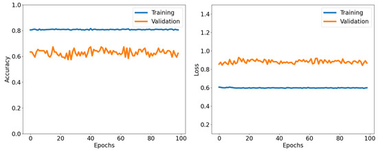
Figure 10.
Accuracy and loss as functions of the number of epochs for both the training and validation datasets in the QCNN. Training with data for and . Accuracy is the mean of the tensor calculated after checking element-wise equality between the true and predicted labels. Accuracy and loss are calculated using Equations (10) and (11).
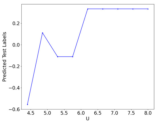
Figure 11.
Predicted test labels vs U. The predicted labels are hovering around zero for . Training with data for and and testing data for .
The exclusive use of high and low values of U during QCNN training has important implications for the identification of quantum critical points. In classical ML, a common technique for detecting phase transitions involves training a supervised model (e.g., a CNN) using control parameters (such as temperature in thermal transitions or external parameters in quantum phase transitions) away from the hypothesized critical point. Our findings indicate that the QCNN can also achieve high accuracy by training on data outside of the hypothesized critical point to predict phases near the critical point [44]. Although the predicted label is worse than the case for which the training data span the entire range of U. However, the average predicted label suggests that the quantum phase transition occurs within the range of . Nonetheless, at the present setting, it does not pinpoint the exact value of U.
8. Discussion
In this work, we present a hybrid quantum–classical algorithm for calculating the phase transition of the Hubbard model under the DMFT approximation. From a practical standpoint, the primary concern is addressing the noise generated by the deep circuit in the Trotter approximation, which affects phase estimation. We did not include the contributions from noise and dissipation in the present study [34]. Recent proposals, in particular, the variational quantum simulation may provide a solution for this problem [99,100]. From a theoretical perspective, the major challenge is properly interpreting the DMFT approximation when implemented with a very limited bath system size. If the bath is restricted to just one or a handful of sites, it may not be clear whether employing the formulation that presumes a continuous distribution of bath sites is either numerically feasible or physically meaningful.
The key quantity for the DMFT, particularly in the two-site approximation, is the quasiparticle weight. The quasiparticle weight can be defined as the measure of damping experienced by the quasiparticle at the Fermi level. At the Fermi level, when the interaction strength is low, the quasiparticle weight is large, which is inversely proportional to the effective mass, indicating free-electron-like behavior, characteristic of a metallic state. As the interaction strength increases, approaching the Mott transition, the quasiparticle weight begins to decrease due to the growing electron correlations. This corresponds to an increase in the effective mass, signaling the gradual suppression of coherent quasiparticles. This behavior is evident in the spectral weight plot (or density of states (DOS) plot), where, in the metallic phase, a sharp quasiparticle peak is observed at the Fermi level. As the interaction increases, this peak gradually diminishes, and at the Mott transition, it vanishes entirely, leaving behind a gap in the spectral function. This indicates the formation of a Mott insulator, where electron localization prevents charge transport, and the system no longer supports well-defined quasiparticle excitations [9]. It is usually calculated using the relation . However, the calculation of self-energy is problematic for a small number of bath sites. This is due to the challenge encountered in solving the Dyson equation for the self-energy . The retarded Green’s function is sensitive to the choice of the imaginary part included in the Fourier transform from time to frequency domains. While this may hold true in general, it is often not a significant factor for systems with a continuous bath - i.e., an infinite number of bath sites. In such systems, the choice of imaginary parts typically does not play a substantial impact on the results, as they remain consistent across a range of choices. The focus of the imaginary part is how to distribute the few delta functions for a limited number of sites [89]. The self-energy obtained from the subtraction of the inverse of the full impurity Green’s function from the inverse of the bare impurity Green’s function cannot be estimated very accurately.
One method suggested is to replace the calculation of from the Dyson equation at the Fermi energy with an averaging of the integration over an energy window centered around the Fermi level [30]. In a way, this approach shifts the problem from selecting the imaginary component in the frequency domain to selecting the integration range over an energy window around the Fermi level. Despite the somewhat arbitrary choice of this range of integration, this method has demonstrated good results [30].
In contrast to many other classical methods used for solving impurity problems, the impurity Green’s function obtained through the VQE and Suzuki–Trotter approximation is expressed in real-time and the computation is limited to ’zero temperature’. This is an inherent advantage of this hybrid quantum–classical approach compared with conventional Monte Carlo-based approaches. This allows us to estimate the self-energy directly from the difference in the inverse of the interacting Green’s function and the bath Green’s function without going to the frequency space. The inverse of Green’s function is more well behaved and less prone to error in numerical calculations.
This approach of calculating the quasiparticle weight directly in the time domain not only avoids the possible ambiguity of choosing the windows of integration but is also more adaptable to a bath with multiple sites. This aligns more broadly with the objective of using hybrid quantum–classical algorithms. The advantage of this approach lies in the fact that we have the information for the self-energy for the full range of the data in the time domain. All the coefficients in the self-energy are calculated and in principle, a full DMFT can be used instead of just the single bath site approximation. In practice, calculations with a large number of bath sites may remain challenging in the near future due to the possibility of increasing errors with larger system sizes. Nevertheless, the formulation presented here can be generalized to calculations with many bath sites.
Besides presenting a modification of the hybrid quantum–classical algorithm for the DMFT, we also tested a new quantity that has not been explored extensively in the context of DMFT [101]. Conventional DMFT is almost always studied at a finite temperature, which may be rather low, but almost never at a true zero temperature for the Hubbard model. This is down to the fact that most existing methods for solving the impurity problems are practically feasible at low though non-zero temperatures. As the wavefunction is explicitly calculated, it is technically at the zero temperature and thus we can meaningfully define the entanglement entropy. The use of entanglement entropy as a witness to phase transition has been studied over the past two decades [102,103,104]. The general feature is that the entanglement entropy increases as the system is tuned close to a phase transition [92]. In the case of the half-filled Hubbard model in the two-site DMFT approach, it is observed that the entanglement entropy reaches its maximum value in the non-interacting limit, but gradually decreases until it saturates once the system enters the Mott insulating phase. A physical interpretation is that in the Mott insulating phase, the bath and the impurity are essentially decoupled, which minimizes the entanglement entropy between them.
For the present problem, the entanglement entropy may not provide much additional insight. However, there are important problems in condensed matter physics for which there is no obvious order parameter. This has been widely discussed in the context of some heavy fermion materials [105]. A method that can detect a putative transition without explicitly constructing an order parameter could be a useful technique.
For capturing the phase transition, we also elaborated on the application of a QML approach to identify phase transitions. The use of ML to locate phase transitions has been well studied. However, using it for the quantum models requires some manipulations of the data, for example, the wavefunctions from exact diagonalization or the Feynman path integral from QMC are inherent quantum data represented in a classical dataset. Various approaches have been proposed and they are quite successful in finding phase transition [44]. Since the data from the VQE are true quantum data, it is natural to use QML. The data can be fed into the quantum classifiers without further manipulation of the data. This is an obvious advantage compared with using the classical ML approach for quantum data. The calculations performed here utilizing the wavefunction derived from DMFT’s converged solution show promising although imperfect results. The performance stagnation observed in the training process of QCNN is due to the inability to effectively capture the intricate variations present in the data associated with phase transitions. The selected training data, limited to U values below and above , do not provide enough representative samples to effectively train the QCNN to recognize the features associated with phase transitions near the critical point. Hence, the model struggles to generalize accurately to unobserved data within this range.
Since using the ML approach to study phase transitions does not require an explicit order parameter, this is advantageous in dealing with crossover problems, where there may not be an explicit order parameter or when the order parameter is unknown. One of them is the crossover between the Fermi liquid and the marginal Fermi liquid [106,107,108]. A thorough study of the entanglement entropy may also provide more insight into this crossover. Perhaps the major difficulty in studying phase transitions using NISQ computers is the rather limited system size. It is reasonable to imagine that even if one can figure out and calculate an order parameter, a proper finite-size scaling as performed in conventional numerical simulations may remain out of reach. An ML-based approach could somehow bypass such difficulties and interpret the finite-size results directly.
9. Conclusions
In summary, we provide a complete workflow for using NISQ to study phase transitions of strongly correlated systems in the thermodynamic limit using the dynamical mean field theory (DMFT). We devise a modification of the hybrid quantum–classical method to solve the DMFT using quantum hardware, first proposed by Kreula et al. [31] and improved by Keen et al. [30] Our modification provides results without arbitrary choices of parameters in estimating the quasiparticle weight. More importantly, it is feasible to be readily generalized for the DMFT with multiple bath sites. With the ground state wavefunction from DMFT, we proposed two approaches to capture phase transitions. The first one is based on calculating the entanglement entropy between the bath sites and the impurity sites. The second one is based on using the wavefunction from the converged solution of DMFT. Both approaches show promising results in identifying the phase transition under the two-site DMFT approximation.
Author Contributions
Conceptualization, K.-M.T.; methodology, A.B., H.F., H.T., K.-M.T. and J.M.; software, A.B. and K.-M.T.; validation, A.B. and K.-M.T.; formal analysis, A.B., H.F., H.T., K.-M.T. and J.M.; investigation, A.B., H.F., H.T., K.-M.T. and J.M.; data curation, A.B.; writing—original draft, A.B. and K.-M.T.; writing—review and editing, H.F., H.T., K.-M.T. and J.M.; supervision, K.-M.T. and J.M.; project administration, K.-M.T. and J.M.; funding acquisition, K.-M.T. and J.M. All authors have read and agreed to the published version of the manuscript.
Funding
This manuscript is based on work supported by NSF DMR-1728457. This work used high-performance computational resources provided by the Louisiana Optical Network Initiative (http://www.loni.org, (accessed on 31 January 2025)) and HPC@LSU computing. HFF is supported by the National Science Foundation under Grant No. PHY-2014023. HT is supported by NSF DMR-1944974 and NSF QIS-2328752 grants. JM is supported by the US Department of Energy, Office of Science, Office of Basic Energy Sciences, under Award Number DE-SC0017861.
Data Availability Statement
The data supporting this study is available upon request to the authors.
Conflicts of Interest
The authors declare no conflicts of interest.
Appendix A
Appendix A.1. Dynamical Mean Field Theory (DMFT)
DMFT generalizes the mean-field theory for classical systems to the quantum fermionic systems on a lattice. As in conventional mean-field theory, it neglects spatial fluctuations; however, it explicitly addresses temporal fluctuations.
The action of the Hubbard model on a lattice in d dimension can be written as
where and are Grassmann variables at space-time point , is the inverse temperature. The quadratic part of the action corresponds to the kinetic energy, characterized by the bare Green’s function which is obtained from the bare dispersion of the Hubbard model. The quartic part corresponds to the interaction from the local coulomb repulsion U.
The exact Green’s function for this action is characterized by the self-energy . In the frequency–momentum space, the Dyson equation gives the relation between the bare Green’s function and the exact Green’s function G:
The full lattice problem, incorporating spatial dependence, is related to a single-site problem through DMFT. The ’cavity method’ rationalizes this approach in the infinite-dimension limit, where all the degrees of freedom, except for a central site, are integrated out as shown in Figure 1a,b. In the limit of , we rescale the hopping amplitude, , ensuring that kinetic energy and interaction energy remain of the same order. The effective action is defined in the frequency domain by
The quadratic part of the impurity action, can be written in terms of the lattice Green’s function for Bethe’s lattice as [8,9,10,11,109]:
Equation (A4) is the self-consistency equation for the DMFT. Green’s function from this action is , are the Matsubara frequencies, which is then fed into the Equation (A4) until the dynamical mean-field, that is, the bath Green’s function, , is converged [9].
The key step of the DMFT algorithm is, given this effective action of the system, to find Green’s function. There are two major types of methods to address this challenge: QMC methods based on sampling the partition function directly or Hamiltonian methods based on the discretization of the electron bath into a finite number of so-called bath sites. For the latter, the DMFT impurity problem can be described by the Anderson impurity model (AIM) or the single-impurity Anderson model (SIAM) defined by the Hamiltonian:
Here, and are creation and annihilation operators for impurity electrons, while and are those of conduction electrons. The action of the Hamiltonian (A5) can be written as that of Equation (A3), with as the non-interacting Anderson impurity model Green’s function, if the number of bath electrons goes to infinity. From now on, without specification, we consider single-particle quantities in real-time or frequency. The frequency , should be understood as . We can connect the lattice Hubbard model and the single-impurity model if we set the self-energy via the condition:
This is fulfilled when we reach the DMFT self-consistency condition [89]:
The hybridization and hopping of conduction electrons on a finite lattice is related to those of the continuum bath via the bare Green’s function as [9,10,11],
with
This Hamiltonian formulation is more convenient for impurity solvers that are based on matrix diagonalization. Such solvers include exact diagonalization [110,111,112], numerical renormalization group [113,114], and other more elaborate methods such as density matrix renormalization group, matrix product state [115,116], and Fock tensor product state [117,118].
Appendix A.2. Two-Site DMFT
The minimal model to mimic the impurity problem is the two-site representation as proposed by Potthoff [89] as shown in Figure 1c. It consists of one site representing the impurity and only one site approximately representing the bath. The SIAM Hamiltonian for one bath site is as follows:
U is the on-site Hubbard interaction at the impurity site denoted as site-1, and is the chemical potential for tuning the electrons filling. and V are the on-site energy of the non-interacting bath site denoted as site-2 and the hybridization between the impurity and the bath site, respectively. For a mapping of the DMFT to the two-site SIAM, the parameters and V are determined iteratively so that the two self-consistency conditions Equations (A14) and (A18) below are satisfied.
In the high-frequency limit, the self-energy of the impurity problem expands in powers of [89]
where is the average occupancy of the impurity orbital:
Inserting the expansion (A11) into (A8) and using Equation (A9), the expansion of the on-site lattice Green’s function is given as
where is the variance of the bare density of states, .
Following Potthoff [89], the first condition is that the electron filling of the impurity site is identified with the filling of the lattice model, i.e.,
where we calculate the band filling using
with and a broadening of .
In the low-frequency limit, the self-energy of the impurity problem is expanded in powers of ,
with a and b as constants. The quasiparticle weight is
Inserting Equations (A16) into (A17), and then neglecting terms of order , yields for small . is the coherent segment of the on-site Green’s function [89]. The second self-consistency condition requires comparing the high-frequency expansions of the respective coherent Green’s functions [89,119],
where . We assume the model is defined in the Bethe lattice with Z nearest neighbors for each site. The Z is set to be infinite, , with . denotes the second moment of the bare density of states. The final equivalence is derived from the semicircular density of states of the Bethe lattice [120].
The primary self-consistency condition holds at lower frequencies up to by considering the weight, the center, and the variance of the coherent quasiparticle peak. Equations (A14) and (A18) reformulate the DMFT self-consistency equation. This is sometimes referred to as linear DMFT [119]. Instead of requiring the self-energy as a function of frequency, the linearized DMFT now involves two equations for fixing and , as these are the only parameters in the effective two-site model. Specifically, for the half-filling two-site case, from Equation (A14) and from Equation (A18). This is much simplified compared with the full DMFT in which Green’s function for each frequency point from the lattice is mapped to that of the impurity.
Appendix A.3. Jordan–Wigner Transformation for Mapping the Fermions to Qubits
We follow the standard Jordan–Wigner transformation to transform the fermionic creation and annihilation operators into spin operators for representation on a quantum computer. A four-qubit system (excluding the ancilla qubit which is used for measurement) is required to represent the two-site SIAM. The spin-down information is encoded by the first two qubits for sites one and two, while the corresponding information for the spin-up occupation is encoded by the third and fourth qubits. The use of Jordan–Wigner transformation to rewrite the Fermionic operators and Green’s function for the two-site model appeared in Kreula et al. [31] and later in Keen et al. [30] The operators are transformed such as:
where, or denote operators on the qubit, while identity operators act on the remaining qubits without explicitly writing them out. The two-site SIAM Hamiltonian is then given by
VQE is employed to find the ground state of the Hamiltonian. Using the first-order Trotter–Suzuki expansion of the time evolution operator acting on the ground state wavefunction to calculate Green’s function in real time. The Trotter–Suzuki transformation is given as
where t is the total time, N is the number of time steps and [121,122,123].
We only focus on the case for the first site. As we only consider the paramagnetic solution of the DMFT, it does not break the spin rotational symmetry. The retarded impurity Green’s function in the time domain is given as [124]
The above equation is recast into spin operators via the Jordan–Wigner transformation. The Green’s functions and can be written as [31,99]
Appendix A.4. Entanglement Entropy
We provide the formulas for calculating the single-site entanglement entropy. For the spin one-half electron system, each site presents four possible local states: . The reduced density matrix for the single site can be written as [92]
with
With the reduced density matrix, the local von Neumann entanglement entropy can be written as
The local entanglement is determined by the combination of four factors, which collectively influence the system’s physical properties [92,93,94]. We can consider the small U and large U limits to have a qualitative understanding of the change in local entanglement as the interaction increases. For small U, the system is in a metal phase in which there are four possible states with the same weight for the impurity site, therefore the reduced density matrix is given by . As we can see in Figure 7, we recovered this value for . On the other hand, in the large U limit, the system is basically classical, because the Hamiltonian is diagonal without the hopping terms. There should be a two-fold degeneracy for a finite system, but it is not expected that the variational wavefunction can capture the degeneracy. The variational wavefunction can only find one of the ground states. Therefore, the entanglement entropy should be zero. As we find in Figure 7, the entanglement entropy is very close to zero once the interaction is above the putative phase transition to the insulating phase.
References
- Varma, C.; Nussinov, Z.; van Saarloos, W. Singular or non-Fermi liquids. Phys. Rep. 2002, 361, 267. [Google Scholar] [CrossRef]
- Savary, L.; Balents, L. Quantum spin liquids: A review. Rep. Prog. Phys. 2016, 80, 016502. [Google Scholar] [CrossRef] [PubMed]
- Stewart, G.R. Heavy-fermion systems. Rev. Mod. Phys. 1984, 56, 755–787. [Google Scholar] [CrossRef]
- Proust, C.; Taillefer, L. The Remarkable Underlying Ground States of Cuprate Superconductors. Annu. Rev. Condens. Matter Phys. 2019, 10, 409–429. [Google Scholar] [CrossRef]
- Varma, C.M. Colloquium: Linear in temperature resistivity and associated mysteries including high temperature superconductivity. Rev. Mod. Phys. 2020, 92, 031001. [Google Scholar] [CrossRef]
- Kanamori, J. Electron correlation and ferromagnetism of transition metals. Prog. Theor. Exp. Phys 1963, 30, 275–289. [Google Scholar]
- Hubbard, J. Electron correlations in narrow energy bands. Proc. Math. Phys. Eng. Sci. 1963, 276, 238–257. [Google Scholar] [CrossRef]
- Georges, A.; Kotliar, G. Hubbard model in infinite dimensions. Phys. Rev. B 1992, 45, 6479. [Google Scholar] [CrossRef]
- Georges, A.; Kotliar, G.; Krauth, W.; Rozenberg, M.J. Dynamical mean-field theory of strongly correlated fermion systems and the limit of infinite dimensions. Rev. Mod. Phys. 1996, 68, 13–125. [Google Scholar] [CrossRef]
- Müller-Hartmann, E. The Hubbard model at high dimensions: Some exact results and weak coupling theory. Z. Phys. B 1989, 76, 211–217. [Google Scholar] [CrossRef]
- Müller-Hartmann, E. Correlated fermions on a lattice in high dimensions. Z. Phys. B 1989, 74, 507–512. [Google Scholar] [CrossRef]
- Metzner, W.; Vollhardt, D. Correlated Lattice Fermions in d=∞ Dimensions. Phys. Rev. Lett. 1989, 62, 324–327. [Google Scholar] [CrossRef]
- Jarrell, M. Hubbard model in infinite dimensions: A quantum Monte Carlo study. Phys. Rev. Lett. 1992, 69, 168–171. [Google Scholar] [CrossRef] [PubMed]
- Toschi, A.; Katanin, A.A.; Held, K. Dynamical vertex approximation: A step beyond dynamical mean-field theory. Phys. Rev. B 2007, 75, 045118. [Google Scholar] [CrossRef]
- Rubtsov, A.N.; Katsnelson, M.I.; Lichtenstein, A.I.; Georges, A. Dual fermion approach to the two-dimensional Hubbard model: Antiferromagnetic fluctuations and Fermi arcs. Phys. Rev. B 2009, 79, 045133. [Google Scholar] [CrossRef]
- Fotso, H.F.; Tam, K.M.; Moreno, J. Beyond quantum cluster theories: Multiscale approaches for strongly correlated systems. Quantum Sci. Technol. 2022, 7, 33001. [Google Scholar] [CrossRef]
- Slezak, C.; Jarrell, M.; Maier, T.; Deisz, J. Multi-scale extensions to quantum cluster methods for strongly correlated electron systems. J. Condens. Matter Phys. 2009, 21, 435604. [Google Scholar] [CrossRef]
- Hague, J.P.; Jarrell, M.; Schulthess, T.C. Fluctuation-exchange supplemented quantum Monte Carlo approach to the Hubbard model. Phys. Rev. B 2004, 69, 165113. [Google Scholar] [CrossRef]
- Rohringer, G.; Hafermann, H.; Toschi, A.; Katanin, A.A.; Antipov, A.E.; Katsnelson, M.I.; Lichtenstein, A.I.; Rubtsov, A.N.; Held, K. Diagrammatic routes to nonlocal correlations beyond dynamical mean field theory. Rev. Mod. Phys. 2018, 90, 025003. [Google Scholar] [CrossRef]
- Hettler, M.H.; Mukherjee, M.; Jarrell, M.; Krishnamurthy, H.R. Dynamical cluster approximation: Nonlocal dynamics of correlated electron systems. Phys. Rev. B 2000, 61, 12739–12756. [Google Scholar] [CrossRef]
- Fotso, H.; Yang, S.; Chen, K.; Pathak, S.; Moreno, J.; Jarrell, M.; Mikelsons, K.; Khatami, E.; Galanakis, D. Dynamical Cluster Approximation. In Strongly Correlated Systems: Theoretical Methods; Avella, A., Mancini, F., Eds.; Springer: Berlin/Heidelberg, Germany, 2012; pp. 271–302. [Google Scholar] [CrossRef]
- Biroli, G.; Kotliar, G. Cluster methods for strongly correlated electron systems. Phys. Rev. B 2002, 65, 155112. [Google Scholar] [CrossRef]
- Knizia, G.; Chan, G.K.L. Density Matrix Embedding: A Simple Alternative to Dynamical Mean-Field Theory. Phys. Rev. Lett. 2012, 109, 186404. [Google Scholar] [CrossRef] [PubMed]
- Arsenault, L.F.; Lopez-Bezanilla, A.; von Lilienfeld, O.A.; Millis, A.J. Machine learning for many-body physics: The case of the Anderson impurity model. Phys. Rev. B 2014, 90, 155136. [Google Scholar] [CrossRef]
- Rigo, J.B.; Mitchell, A.K. Machine learning effective models for quantum systems. Phys. Rev. B 2020, 101, 241105. [Google Scholar] [CrossRef]
- Sheridan, E.; Rhodes, C.; Jamet, F.; Rungger, I.; Weber, C. Data-driven dynamical mean-field theory: An error-correction approach to solve the quantum many-body problem using machine learning. Phys. Rev. B 2021, 104, 205120. [Google Scholar] [CrossRef]
- Walker, N.; Kellar, S.; Zhang, Y.; Tam, K.M.; Moreno, J. Neural Network Solver for Small Quantum Clusters. Crystals 2022, 12, 1269. [Google Scholar] [CrossRef]
- Sturm, E.J.; Carbone, M.R.; Lu, D.; Weichselbaum, A.; Konik, R.M. Predicting impurity spectral functions using machine learning. Phys. Rev. B 2021, 103, 245118. [Google Scholar] [CrossRef]
- Bauer, B.; Wecker, D.; Millis, A.J.; Hastings, M.B.; Troyer, M. Hybrid Quantum-Classical Approach to Correlated Materials. Phys. Rev. X 2016, 6, 031045. [Google Scholar] [CrossRef]
- Keen, T.; Maier, T.; Johnston, S.; Lougovski, P. Quantum-classical simulation of two-site dynamical mean-field theory on noisy quantum hardware. Quantum Sci. Technol. 2020, 5, 035001. [Google Scholar] [CrossRef]
- Kreula, J.M.; García-Álvarez, L.; Lamata, L.; Clark, S.R.; Solano, E.; Jaksch, D. Few-qubit quantum-classical simulation of strongly correlated lattice fermions. EPJ Quantum Technol. 2016, 3, 11. [Google Scholar] [CrossRef]
- Steckmann, T.; Keen, T.; Kökcü, E.; Kemper, A.F.; Dumitrescu, E.F.; Wang, Y. Mapping the metal-insulator phase diagram by algebraically fast-forwarding dynamics on a cloud quantum computer. Phys. Rev. Res. 2023, 5, 023198. [Google Scholar] [CrossRef]
- Jaderberg, B. Solving Optimisation Problems on Near-Term Quantum Computers. Ph.D. Thesis, University of Oxford, Oxford, UK, 2022. [Google Scholar]
- Rungger, I.; Fitzpatrick, N.; Chen, H.; Alderete, C.H.; Apel, H.; Cowtan, A.; Patterson, A.; Ramo, D.M.; Zhu, Y.; Nguyen, N.H.; et al. Dynamical Mean Field Theory Algorithm and Experiment on Quantum Computers. Quantum Sci. Technol. 2021, 6, 025004. [Google Scholar] [CrossRef]
- Jaderberg, B.; Agarwal, A.; Leonhardt, K.; Kiffner, M.; Jaksch, D. Minimum hardware requirements for hybrid quantum–classical DMFT. Quantum Sci. Technol. 2020, 5, 034015. [Google Scholar]
- Johnston, S.; Khatami, E.; Scalettar, R. A perspective on machine learning and data science for strongly correlated electron problems. Carbon Trends 2022, 9, 100231. [Google Scholar]
- Wang, L. Discovering phase transitions with unsupervised learning. Phys. Rev. B 2016, 94, 195105. [Google Scholar] [CrossRef]
- Wetzel, S.J. Unsupervised learning of phase transitions: From principal component analysis to variational autoencoders. Phys. Rev. E 2017, 96, 022140. [Google Scholar]
- van Nieuwenburg, E.P.L.; Liu, Y.H.; Huber, S.D. Learning phase transitions by confusion. Nat. Phys 2017, 13, 435–439. [Google Scholar] [CrossRef]
- Cassella, G.; Sutterud, H.; Azadi, S.; Drummond, N.D.; Pfau, D.; Spencer, J.S.; Foulkes, W.M.C. Discovering Quantum Phase Transitions with Fermionic Neural Networks. Phys. Rev. Lett. 2023, 130, 036401. [Google Scholar] [CrossRef]
- Dong, X.Y.; Pollmann, F.; Zhang, X.F. Machine learning of quantum phase transitions. Phys. Rev. B 2019, 99, 121104. [Google Scholar] [CrossRef]
- Hu, W.; Singh, R.R.P.; Scalettar, R.T. Discovering phases, phase transitions, and crossovers through unsupervised machine learning: A critical examination. Phys. Rev. E 2017, 95, 062122. [Google Scholar] [CrossRef]
- Walker, N.; Tam, K.M.; Novak, B.; Jarrell, M. Identifying structural changes with unsupervised machine learning methods. Phys. Rev. E 2018, 98, 053305. [Google Scholar] [CrossRef]
- Carrasquilla, J.; Melko, R.G. Machine learning phases of matter. Nat. Phys. 2017, 13, 431–434. [Google Scholar] [CrossRef]
- Wetzel, S.J.; Scherzer, M. Machine learning of explicit order parameters: From the Ising model to SU (2) lattice gauge theory. Phys. Rev. B 2017, 96, 184410. [Google Scholar] [CrossRef]
- Walker, N.; Tam, K.M. InfoCGAN classification of 2D square Ising configurations. Mach. Learn. Sci. Technol. 2020, 2, 025001. [Google Scholar]
- Zhang, Y.; Mesaros, A.; Fujita, K.; Edkins, S.D.; Hamidian, M.H.; Ch’ng, K.; Eisaki, H.; Uchida, S.; Davis, J.C.S.; Khatami, E.; et al. Machine learning in electronic-quantum-matter imaging experiments. Nature 2019, 570, 484–490. [Google Scholar] [CrossRef]
- Lozano-Gómez, D.; Pereira, D.; Gingras, M.J.P. Unsupervised machine learning of quenched gauge symmetries: A proof-of-concept demonstration. Phys. Rev. Res. 2022, 4, 043118. [Google Scholar] [CrossRef]
- Mano, T.; Ohtsuki, T. Phase Diagrams of Three-Dimensional Anderson and Quantum Percolation Models Using Deep Three-Dimensional Convolutional Neural Network. J. Phys. Soc. Jpn. 2017, 86, 113704. [Google Scholar] [CrossRef]
- Beach, M.J.S.; Golubeva, A.; Melko, R.G. Machine learning vortices at the Kosterlitz-Thouless transition. Phys. Rev. B 2018, 97, 045207. [Google Scholar] [CrossRef]
- Khatami, E.; Guardado-Sanchez, E.; Spar, B.M.; Carrasquilla, J.F.; Bakr, W.S.; Scalettar, R.T. Visualizing strange metallic correlations in the two-dimensional Fermi-Hubbard model with artificial intelligence. Phys. Rev. A 2020, 102, 033326. [Google Scholar] [CrossRef]
- Baul, A.; Walker, N.; Moreno, J.; Tam, K.M. Application of the variational autoencoder to detect the critical points of the anisotropic Ising model. Phys. Rev. E 2023, 107, 045301. [Google Scholar] [CrossRef]
- Monaco, S.; Kiss, O.; Mandarino, A.; Vallecorsa, S.; Grossi, M. Quantum phase detection generalization from marginal quantum neural network models. Phys. Rev. B 2023, 107, L081105. [Google Scholar] [CrossRef]
- Peral-García, D.; Cruz-Benito, J.; García-Peñalvo, F.J. Systematic literature review: Quantum machine learning and its applications. Comput. Sci. Rev. 2024, 51, 100619. [Google Scholar] [CrossRef]
- Wrobel, N.; Baul, A.; Tam, K.M.; Moreno, J. Detecting Quantum Critical Points of Correlated Systems by Quantum Convolutional Neural Network Using Data from Variational Quantum Eigensolver. Quantum Rep. 2022, 4, 574–588. [Google Scholar] [CrossRef]
- Chollet, F.; Gardener, T.; Zhu, Q.S.; Jin, H.; Rahman, F.; Chiu, H.; Watson, M.; Qian, C.; Lee, T.; de Marmiesse, G.; et al. Keras. Available online: https://github.com/fchollet/keras (accessed on 13 May 2015).
- Abadi, M.; Agarwal, A.; Barham, P.; Brevdo, E.; Chen, Z.; Citro, C.; Corrado, G.S.; Davis, A.; Dean, J.; Devin, M.; et al. TensorFlow: Large-Scale Machine Learning on Heterogeneous Systems. 2015. Available online: https://tensorflow.org (accessed on 17 November 2015).
- Lloyd, S.; Mohseni, M.; Rebentrost, P. Quantum Algorithms for Fixed Qubit Architectures. Nat. Phys. 2014, 10, 631–633. [Google Scholar] [CrossRef]
- Pastorello, D. Quantum Classification. In Concise Guide to Quantum Machine Learning; Springer Nature: Singapore, 2023; pp. 69–87. [Google Scholar] [CrossRef]
- Huang, H.Y.; Broughton, M.; Mohseni, M.; Babbush, R.; Boixo, S.; Neven, H.; McClean, J.R. Power of data in quantum machine learning. Nat. Commun. 2021, 12, 2631. [Google Scholar] [CrossRef] [PubMed]
- Cappelletti, W.; Erbanni, R.; Keller, J. Polyadic Quantum Classifier. In Proceedings of the 2020 IEEE International Conference on Quantum Computing and Engineering (QCE), Denver, CO, USA, 12–16 October 2020; pp. 22–29. [Google Scholar] [CrossRef]
- Belis, V.; González-Castillo, S.; Reissel, C.; Vallecorsa, S.; Combarro, E.F.; Dissertori, G.; Reiter, F. Higgs analysis with quantum classifiers. In Proceedings of the 25th International Conference on Computing in High Energy and Nuclear Physics (CHEP 2021), Virtual, 17–21 May 2021; EDP Sciences: Les Ulis, France, 2021; Volume 251, p. 03070. [Google Scholar]
- Sen, P.; Bhatia, A.S.; Bhangu, K.S.; Elbeltagi, A. Variational quantum classifiers through the lens of the Hessian. PLoS ONE 2022, 17, e0262346. [Google Scholar] [CrossRef]
- Park, D.K.; Blank, C.; Petruccione, F. Robust quantum classifier with minimal overhead. In Proceedings of the 2021 International Joint Conference on Neural Networks, IJCNN, Shenzhen, China, 18–22 July 2021; IEEE: New York, NY, USA, 2021; pp. 1–7. [Google Scholar]
- Blank, C.; Park, D.K.; Rhee, J.K.K.; Petruccione, F. Quantum classifier with tailored quantum kernel. npj Quantum Inf. 2020, 6, 41. [Google Scholar] [CrossRef]
- Schuld, M.; Bocharov, A.; Svore, K.M.; Wiebe, N. Circuit-centric quantum classifiers. Phys. Rev. A 2020, 101, 032308. [Google Scholar] [CrossRef]
- Miyahara, H.; Roychowdhury, V. Ansatz-Independent Variational Quantum Classifiers and the Price of Ansatz. Sci. Rep. 2022, 12, 19520. [Google Scholar]
- Blance, A.; Spannowsky, M. Quantum machine learning for particle physics using a variational quantum classifier. J. High Energy Phys. 2021, 2021, 212. [Google Scholar] [CrossRef]
- Grant, E.; Benedetti, M.; Cao, S.; Hallam, A.; Lockhart, J.; Stojevic, V.; Green, A.G.; Severini, S. Hierarchical quantum classifiers. npj Quantum Inf. 2018, 4, 65. [Google Scholar]
- LaRose, R.; Coyle, B. Robust data encodings for quantum classifiers. Phys. Rev. A 2020, 102. [Google Scholar] [CrossRef]
- Du, Y.; Hsieh, M.H.; Liu, T.; Tao, D.; Liu, N. Quantum noise protects quantum classifiers against adversaries. Phys. Rev. Res. 2021, 3, 023153. [Google Scholar]
- Abohashima, Z.; Elhoseny, M.; Houssein, E.H.; Mohamed, W.M. Classification with Quantum Machine Learning: A Survey. Quant. Inf. Process. 2020, 19, 1–26. [Google Scholar] [CrossRef]
- Chen, S.Y.C.; Huang, C.M.; Hsing, C.W.; Kao, Y.J. Hybrid Quantum-Classical Classifier Based on Tensor Network and Variational Quantum Circuit. IEEE Trans. Quantum Eng. 2020, 1, 1–9. [Google Scholar]
- Farhi, E.; Neven, H. Classification with Quantum Neural Networks on Near Term Processors. Nat. Mach. Intell. 2019, 1, 246–250. [Google Scholar] [CrossRef]
- Lecun, Y.; Bottou, L.; Bengio, Y.; Haffner, P. Gradient-based learning applied to document recognition. Proc. IEEE 1998, 86, 2278–2324. [Google Scholar] [CrossRef]
- Bény, C. Deep Learning and the Renormalization Group. Quantum Inf. Process. 2013, 12, 2023–2048. [Google Scholar] [CrossRef]
- Mehta, P.; Schwab, D.J. An Exact Mapping Between the Variational Renormalization Group and Deep Learning. Phys. Rev. X 2015, 5, 041019. [Google Scholar] [CrossRef]
- Lin, H.W.; Tegmark, M.; Rolnick, D. Why Does Deep and Cheap Learning Work So Well? J. Stat. Phys. 2017, 168, 1223–1247. [Google Scholar] [CrossRef]
- Koch, E.D.M.; Koch, R.D.M.; Cheng, L. Is Deep Learning a Renormalization Group Flow? IEEE Access 2020, 8, 106487–106505. [Google Scholar] [CrossRef]
- Funai, S.S.; Giataganas, D. Thermodynamics and feature extraction by machine learning. Phys. Rev. Res. 2020, 2, 033415. [Google Scholar]
- Iso, S.; Shiba, S.; Yokoo, S. Scale-invariant feature extraction of neural network and renormalization group flow. Phys. Rev. E 2018, 97, 053304. [Google Scholar] [CrossRef]
- Koch-Janusz, M.; Ringel, Z. Mutual information, neural networks and the renormalization group. Nat. Phys. 2018, 14, 578–582. [Google Scholar] [CrossRef]
- Ch’Ng, K.; Carrasquilla, J.; Melko, R.G.; Khatami, E. Machine learning phases of strongly correlated fermions. Phys. Rev. X 2017, 7, 031038. [Google Scholar] [CrossRef]
- Carleo, G.; Cirac, I.; Cranmer, K.; Daudet, L.; Schuld, M.; Tishby, N.; Vogt-Maranto, L.; Zdeborová, L. Machine learning and the physical sciences. Rev. Mod. Phys. 2019, 91, 045002. [Google Scholar] [CrossRef]
- Cong, I.; Choi, S.; Lukin, M.D. Quantum convolutional neural networks. Nat. Phys 2019, 15, 1273–1278. [Google Scholar] [CrossRef]
- Uvarov, A.V.; Kardashin, A.S.; Biamonte, J.D. Machine learning phase transitions with a quantum processor. Phys. Rev. A 2020, 102, 012415. [Google Scholar]
- Tibaldi, S.; Magnifico, G.; Vodola, D.; Ercolessi, E. Unsupervised and supervised learning of interacting topological phases from single-particle correlation functions. SciPost Phys. 2023, 14, 005. [Google Scholar] [CrossRef]
- Schindler, F.; Regnault, N.; Neupert, T. Probing many-body localization with neural networks. Phys. Rev. B 2017, 95, 245134. [Google Scholar] [CrossRef]
- Potthoff, M. Two-site dynamical mean-field theory. Phys. Rev. B 2001, 64, 165114. [Google Scholar] [CrossRef]
- Tilly, J.; Chen, H.; Cao, S.; Picozzi, D.; Setia, K.; Li, Y.; Grant, E.; Wossnig, L.; Rungger, I.; Booth, G.H.; et al. The Variational Quantum Eigensolver: A review of methods and best practices. Phys. Rep. 2022, 986, 1–128. [Google Scholar] [CrossRef]
- Dorner, R.; Clark, S.R.; Heaney, L.; Fazio, R.; Goold, J.; Vedral, V. Extracting Quantum Work Statistics and Fluctuation Theorems by Single-Qubit Interferometry. Phys. Rev. Lett. 2013, 110, 230601. [Google Scholar] [CrossRef] [PubMed]
- Gu, S.J.; Deng, S.S.; Li, Y.Q.; Lin, H.Q. Entanglement and Quantum Phase Transition in the Extended Hubbard Model. Phys. Rev. Lett. 2004, 93, 086402. [Google Scholar] [CrossRef]
- Deng, S.S.; Gu, S.J.; Lin, H.Q. Block-block entanglement and quantum phase transitions in the one-dimensional extended Hubbard model. Phys. Rev. B 2006, 74, 045103. [Google Scholar] [CrossRef]
- Spalding, J.; Tsai, S.W.; Campbell, D.K. Critical entanglement for the half-filled extended Hubbard model. Phys. Rev. B 2019, 99, 195445. [Google Scholar] [CrossRef]
- Schuld, M.; Petruccione, F. Quantum Models as Kernel Methods. In Machine Learning with Quantum Computers; Springer International Publishing: Cham, Switzerland, 2021; pp. 217–245. [Google Scholar] [CrossRef]
- Beer, K.; Bondarenko, D.; Farrelly, T.; Osborne, T.J.; Salzmann, R.; Scheiermann, D.; Wolf, R. Training deep quantum neural networks. Nat. Commun. 2020, 11, 808. [Google Scholar]
- Lippmann, R. Book review: “Neural networks, a comprehensive foundation”, by Simon Haykin. Int. J. Neural Syst. 1994, 5, 363–364. [Google Scholar]
- Agostinelli, F.; Hoffman, M.; Sadowski, P.; Baldi, P. Learning Activation Functions to Improve Deep Neural Networks. Neurocomputing 2017, 267, 42–51. [Google Scholar] [CrossRef]
- Endo, S.; Kurata, I.; Nakagawa, Y.O. Calculation of the Green’s function on near-term quantum computers. Phys. Rev. Res. 2020, 2, 033281. [Google Scholar] [CrossRef]
- Sakurai, R.; Mizukami, W.; Shinaoka, H. Hybrid quantum-classical algorithm for computing imaginary-time correlation functions. Phys. Rev. Res. 2022, 4, 023219. [Google Scholar] [CrossRef]
- Su, D.D.; Dai, X.; Tong, N.H. Local Entanglement Entropy at the Mott Metal-Insulator Transition in Infinite Dimensions. Mod. Phys. Lett. B 2013, 27, 1350034. [Google Scholar] [CrossRef]
- Sachdev, S. Quantum phase transitions. Phys. World 1999, 12, 33. [Google Scholar]
- Osborne, T.J.; Nielsen, M.A. Entanglement, quantum phase transitions, and density matrix renormalization. Quantum Inf. Process. 2002, 1, 45–53. [Google Scholar] [CrossRef]
- Osterloh, A.; Amico, L.; Falci, G.; Fazio, R. Scaling of entanglement close to a quantum phase transition. Nature 2002, 416, 608–610. [Google Scholar] [CrossRef]
- Haule, K.; Kotliar, G. Arrested Kondo effect and hidden order in URu2Si2. Nat. Phys. 2009, 5, 796–799. [Google Scholar] [CrossRef]
- Vidhyadhiraja, N.S.; Macridin, A.; Şen, C.; Jarrell, M.; Ma, M. Quantum Critical Point at Finite Doping in the 2D Hubbard Model: A Dynamical Cluster Quantum Monte Carlo Study. Phys. Rev. Lett. 2009, 102, 206407. [Google Scholar] [CrossRef] [PubMed]
- Kellar, S.; Tam, K.M.; Moreno, J. Non-Fermi Liquid Behavior in the Three-Dimensional Hubbard Model. Crystals 2023, 13, 106. [Google Scholar] [CrossRef]
- Yang, S.X.; Fotso, H.; Su, S.Q.; Galanakis, D.; Khatami, E.; She, J.H.; Moreno, J.; Zaanen, J.; Jarrell, M. Proximity of the Superconducting Dome and the Quantum Critical Point in the Two-Dimensional Hubbard Model. Phys. Rev. Lett. 2011, 106, 047004. [Google Scholar] [CrossRef]
- Maier, T.; Jarrell, M.; Pruschke, T.; Hettler, M.H. Quantum cluster theories. Rev. Mod. Phys. 2005, 77, 1027. [Google Scholar]
- Caffarel, M.; Krauth, W. Exact diagonalization approach to correlated fermions in infinite dimensions: Mott transition and superconductivity. Phys. Rev. Lett. 1994, 72, 1545–1548. [Google Scholar] [CrossRef]
- Capone, M.; de’ Medici, L.; Georges, A. Solving the dynamical mean-field theory at very low temperatures using the Lanczos exact diagonalization. Phys. Rev. B 2007, 76, 245116. [Google Scholar] [CrossRef]
- Liebsch, A.; Ishida, H. Temperature and bath size in exact diagonalization dynamical mean field theory. J. Phys. Soc. Jpn. 2011, 24, 053201. [Google Scholar] [CrossRef] [PubMed]
- Bulla, R.; Costi, T.A.; Pruschke, T. Numerical renormalization group method for quantum impurity systems. Rev. Mod. Phys. 2008, 80, 395–450. [Google Scholar] [CrossRef]
- Peters, R.; Pruschke, T.; Anders, F.B. Numerical renormalization group approach to Green’s functions for quantum impurity models. Phys. Rev. B 2006, 74, 245114. [Google Scholar] [CrossRef]
- Ganahl, M.; Aichhorn, M.; Evertz, H.G.; Thunström, P.; Held, K.; Verstraete, F. Efficient DMFT impurity solver using real-time dynamics with matrix product states. Phys. Rev. B 2015, 92, 155132. [Google Scholar] [CrossRef]
- Wolf, F.A.; Justiniano, J.A.; McCulloch, I.P.; Schollwöck, U. Spectral functions and time evolution from the Chebyshev recursion. Phys. Rev. B 2015, 91, 115144. [Google Scholar] [CrossRef]
- Bauernfeind, D.; Zingl, M.; Triebl, R.; Aichhorn, M.; Evertz, H.G. Fork Tensor-Product States: Efficient Multiorbital Real-Time DMFT Solver. Phys. Rev. X 2017, 7, 031013. [Google Scholar] [CrossRef]
- Weh, A.; Zhang, Y.; Östlin, A.; Terletska, H.; Bauernfeind, D.; Tam, K.M.; Evertz, H.G.; Byczuk, K.; Vollhardt, D.; Chioncel, L. Dynamical mean-field theory of the Anderson-Hubbard model with local and nonlocal disorder in tensor formulation. Phys. Rev. B 2021, 104, 045127. [Google Scholar] [CrossRef]
- Bulla, R.; Potthoff, M. “Linearized” dynamical mean-field theory for the Mott-Hubbard transition. Eur. Phys. J. B 2000, 13, 257–264. [Google Scholar] [CrossRef]
- Bethe, H.A. Statistical theory of superlattices. Proc. R. Soc. Lond. Ser. A 1935, 150, 552–575. [Google Scholar]
- Vidal, G.; Dawson, C.M. Universal quantum circuit for two-qubit transformations with three controlled-NOT gates. Phys. Rev. A 2004, 69, 010301. [Google Scholar] [CrossRef]
- Coffey, M.W.; Deiotte, R.; Semi, T. Comment on “Universal quantum circuit for two-qubit transformations with three controlled-NOT gates” and “Recognizing small-circuit structure in two-qubit operators”. Phys. Rev. A 2008, 77, 066301. [Google Scholar] [CrossRef]
- Klco, N.; Dumitrescu, E.F.; McCaskey, A.J.; Morris, T.D.; Pooser, R.C.; Sanz, M.; Solano, E.; Lougovski, P.; Savage, M.J. Quantum-classical computation of Schwinger model dynamics using quantum computers. Phys. Rev. A 2018, 98, 032331. [Google Scholar] [CrossRef]
- Freericks, J.K. An Introduction to Many-Body Green’s Functions in and out of Equilibrium. Adv. Phys. 2020, 69, 3–32. [Google Scholar] [CrossRef]


Disclaimer/Publisher’s Note: The statements, opinions and data contained in all publications are solely those of the individual author(s) and contributor(s) and not of MDPI and/or the editor(s). MDPI and/or the editor(s) disclaim responsibility for any injury to people or property resulting from any ideas, methods, instructions or products referred to in the content. |
© 2025 by the authors. Licensee MDPI, Basel, Switzerland. This article is an open access article distributed under the terms and conditions of the Creative Commons Attribution (CC BY) license (https://creativecommons.org/licenses/by/4.0/).