Instability of Meissner Differential Equation and Its Relation with Photon Excitations and Entanglement in a System of Coupled Quantum Oscillators

Abstract

In this work, we investigate the Schrödinger dynamics of photon excitation numbers and entanglement in a system composed by two non-resonant time-dependent coupled oscillators. By considering $\pi$ periodically pumped parameters (oscillator frequencies and coupling) and using suitable transformations, we show that the quantum dynamics can be determined by two classical Meissner oscillators. We then study analytically the stability of these differential equations and the dynamics of photon excitations and entanglement in the quantum system numerically. Our analysis shows two interesting results, which can be summarized as follows: (i) Classical instability of classical analog of quantum oscillators and photon excitation numbers (expectations $⟨N_j⟩$) are strongly correlated, and (ii) photon excitations and entanglement are connected to each other. These results can be used to shed light on the link between quantum systems and their classical counterparts and provide a nice complement to the existing works studying the dynamics of coupled quantum oscillators.

1. Introduction

Quantum entanglement is one of the most intriguing concepts of quantum theory [1,2], although it was initially conceptualized and used to refute the basic quantum principles. Indeed, Einstein, Podolsky and Rosen have argued against some results of quantum theory by remarking that the wave functions can be entangled, which entails in their point of view the existence of hidden variables [1,3]. It was later realized that entanglement is an essential component of quantum theory because, without it, it is impossible to interpret and confirm the provisions of the theory [4]. Nowadays, it is widely understood that entanglement plays an important role in quantum information processing protocols, and it is considered a necessary resource to go beyond classical communications and technologies.

During the last years, controlling entanglement in systems of time-dependent coupled harmonic oscillators has been extensively studied [3,5,6,7,8,9,10,11]. These investigations were also motivated by experiments providing access to the ultra strong coupling (USC) regime [12,13], where the coupling is comparable to the transition frequencies of the coupled quantum systems. In another work, it was shown that it is possible to generate entanglement by phasing control in two [14] and three [15] isotropic harmonic oscillators sinusoidally coupled to each other by $J\left(t\right)=J_{0}cos\left(\omega t\right)$ and weakly coupled to a harmonic bath. It was also found that the survival of entanglement for large simulation times is due to the instability of decoupled from the bath normal oscillator modes [3]. The connection between normal mode instability and entanglement growth was also demonstrated in References [16,17], again by using sinusoidal coupling. More recently, it was shown in Reference [18] that the ground state $|G\rangle$ of two time-independent resonant oscillators contains, in the USC regime, virtual (cannot be absorbed) excitations VE, i.e., $\langle G|N_1|G\rangle =\langle G|N_2|G\rangle \ne 0$, with $N_1$ and $N_2$ being the photon number operators corresponding to the coupled oscillators. Note that the term VE is used here to denote virtual photons that exist in the ground state but cannot be detected directly [18], although there are some proposals in order to probe them [19,20]. This is not to be confused with the usage of the term in several other works [21,22,23,24,25] in which qubits detuned from a cavity where they are embedded and interact through the virtual exchange of photons with the cavity. In the weak coupling regime, the ground state of the two coupled oscillatos is empty and does not contain VE, but as the coupling increases and reaches USC it becomes populated [13]. VEs were considered as a consequence of the counter-rotating terms appearing in the Hamiltonian of coupled oscillators, and the maintenance of entanglement between oscillators was attributed to the presence of these excitations.

Motivated by the above studies, in the present work we elucidate the interplay between the instability of classical oscillator equations, which can be associated with the system of time-dependent coupled quantum oscillators under study, the virtual quantum excitations and quantum entanglement. Specifically, we address the question of how classical instabilities affect photon excitations and consequently result in entanglement in the ground state of two time-dependent non-resonant coupled harmonic oscillators. We make these investigations by using a pair of harmonic oscillators connected by a periodically quenched coupling parameter $J\left(t\right)=J_0\mathsf{\Theta }\left(t\right)$ and with time-dependent frequencies ${\omega }_{1,2}^2\left(t\right)={\omega }_0^2\pm ϵ\mathsf{\Theta }\left(t\right)$, where $\mathsf{\Theta }$ is a $\pi$-periodic square wave with alternating value $\pm 1$, and $ϵ$ is the quench amplitude. Under this choice of time-dependent functions, the resolution of Schrödinger dynamics allows us to find Ermakov equations [26], and the utilization of suitable transformations results in two Meissner differential equations [27] corresponding to classical counterparts of the decoupled Hamiltonian. Then, we study the instabilities of the derived differential equations and obtain stability-instability diagrams, which enable us to investigate the link between two strongly different features, VEs and classical instabilities. Additionally, by computing logarithmic negativity, we establish the relation between entanglement and VE.

The layout of our paper is as follows. In Section 2, we present our coupled oscillator model and show how to exactly decouple the Hamiltonian system by using suitable transformations. The instabilities of Ermakov and Meissner equations emerging from the analysis are discussed in Section 3. In Section 4, we quantify entanglement by using logarithmic negativity and calculate the VE in both oscillators by averaging the number operators over the ground state. In Section 5, we present numerical results for various values of system parameters and discuss the interplay between these phenomena. Finally, Section 6 concludes this work.

2. Model and Schrödinger Dynamics

2.1. Model and Integrability

The model under study is displayed in Figure 1 and consists of two time-dependent non-resonant coupled harmonic oscillators described by the following Hamiltonian:

$$\begin{array}{c}\hfill H({\widehat{x}}_1,{\widehat{x}}_2)=\frac{{\widehat{p}}_1^2}{2}+\frac{{\widehat{p}}_2^2}{2}+\frac{1}{2}{\omega }_1^2\left(t\right){\widehat{x}}_1^2+\frac{1}{2}{\omega }_2^2\left(t\right){\widehat{x}}_2^2-J\left(t\right){\widehat{x}}_1{\widehat{x}}_2,\end{array}$$

(1)

where positions $\widehat{x_j}$ and momenta ${\widehat{p}}_k$ and $j,k=1,2$ satisfy the canonical commutation relations $\left[{\widehat{x}}_j,{\widehat{p}}_k\right]=i{\delta }_{jk}$; ${\omega }_j\left(t\right)$ is the time-dependent frequencies of the oscillators; and $J\left(t\right)$ is the time-dependent coupling parameter between them. For the sake of simplicity, we assume unit masses (a transformation that may be applied to the more general case and make this assumption valid [28,29]) and $\hslash =1$.

Since the time-dependent Hamiltonian (1) involves an interaction term, a straightforward diagonalization is not an easy task. In order to overcome this, we introduce the following time-dependent rotation by the angle $\alpha \left(t\right)$ defined below:

$$\begin{array}{c}\hfill {\mathcal{R}}_{\alpha }\left(t\right)=exp[-i\alpha \left(t\right){\widehat{L}}_z],\alpha \left(t\right)=\frac{1}{2}arctan\left(\frac{2J\left(t\right)}{{\omega }_1^2\left(t\right)-{\omega }_2^2\left(t\right)}\right),\end{array}$$

(2)

where ${\widehat{L}}_z={\widehat{x}}_1{\widehat{p}}_2-{\widehat{x}}_2{\widehat{p}}_1$ is the angular momentum operator. The transformed Hamiltonian is given by the following:

$$\begin{array}{c}\hfill \tilde{H}({\widehat{x}}_1,{\widehat{x}}_2)={\mathcal{R}}_{\alpha }\left(t\right)H({\widehat{x}}_1,{\widehat{x}}_2){\mathcal{R}}_{\alpha }^{-1}\left(t\right)-i{\mathcal{R}}_{\alpha }\left(t\right){\partial }_t{\mathcal{R}}_{\alpha }^{-1}\left(t\right),\end{array}$$

(3)

and after some algebra we obtain the following:

$$\begin{array}{c}\hfill \tilde{H}({\widehat{x}}_1,{\widehat{x}}_2)=\frac{{\widehat{p}}_1^2}{2}+\frac{{\widehat{p}}_2^2}{2}+\frac{1}{2}{\mathsf{\Omega }}_1^2\left(t\right){\widehat{x}}_1^2+\frac{1}{2}{\mathsf{\Omega }}_2^2\left(t\right){\widehat{x}}_2^2+\dot{\alpha }\left(t\right)({\widehat{x}}_1{\widehat{p}}_2-{\widehat{x}}_2{\widehat{p}}_1),\end{array}$$

(4)

where the frequencies ${\mathsf{\Omega }}_j$ are defined as follows.

$$\begin{array}{ccc}\hfill {\mathsf{\Omega }}_1^2\left(t\right)& =& {\omega }_1^2\left(t\right){cos}^2\alpha +{\omega }_2^2\left(t\right){sin}^2\alpha +2J\left(t\right)sin\alpha cos\alpha ,\hfill \end{array}$$

(5a)

$$\begin{array}{ccc}\hfill {\mathsf{\Omega }}_2^2\left(t\right)& =& {\omega }_1^2\left(t\right){sin}^2\alpha +{\omega }_2^2\left(t\right){cos}^2\alpha -2J\left(t\right)sin\alpha cos\alpha .\hfill \end{array}$$

(5b)

For the boundness of this Hamiltonian, it is required that ${\mathsf{\Omega }}_j^2>0$. From Equation (4), it becomes obvious that the separation of variables is possible for $\dot{\alpha }\left(t\right)=0$, and by using Equation (2), this condition results in the following relation:

$$tan\left(2\alpha \left(t\right)\right)=\frac{2J\left(t\right)}{{\omega }_1^2\left(t\right)-{\omega }_2^2\left(t\right)}=constant,$$

(6)

which has been also used in different occasions, see for instance References [28,30]. The original Hamiltonian is, thus, canonically equivalent to the following decoupled Hamiltonian:

$$\begin{array}{c}\hfill \tilde{H}({\widehat{x}}_1,{\widehat{x}}_2)=\frac{{\widehat{p}}_1^2}{2}+\frac{1}{2}{\mathsf{\Omega }}_1^2\left(t\right){\widehat{x}}_1^2+\frac{{\widehat{p}}_2^2}{2}+\frac{1}{2}{\mathsf{\Omega }}_2^2\left(t\right){\widehat{x}}_2^2={\tilde{H}}_1\left(\widehat{x_1}\right)+{\tilde{H}}_2\left(\widehat{x_2}\right),\end{array}$$

(7)

which can be easily solved.

2.2. Time-Dependent Schrödinger Equation

The commutation relation $\left[{\tilde{H}}_1,{\tilde{H}}_2\right]=0$ implies that the solutions of the time-dependent Schrödinger equation corresponding to the decoupled Hamiltonian (7) have the following form:

$$\begin{array}{c}\hfill \tilde{\mathsf{\Psi }}(x_1,x_2;t)={\tilde{\varphi }}_1(x_1;t)\otimes {\tilde{\varphi }}_2(x_2;t)\end{array}$$

(8)

where each $\tilde{\varphi }(x_j;t)$ satisfies the corresponding single-particle Schrödinger equation.

$$\begin{array}{c}\hfill \left(-\frac{1}{2}{\partial }_{x_j}^2+\frac{1}{2}{\mathsf{\Omega }}_j^2\left(t\right){\widehat{x}}_j^2\right)\widetilde{{\varphi }_j}(x_j;t)=i{\partial }_t{\tilde{\varphi }}_j(x_j;t),j=1,2.\end{array}$$

(9)

This equation was studied earlier in References [31,32,33], where the general solution was derived as a superposition of orthonormal expanding modes $\tilde{\psi }(x_j;t)={\displaystyle \sum _{n_j=0}}{\mathfrak{p}}_{n_j}\left(t\right){\tilde{\varphi }}_j(x_j,t)$, with ${\displaystyle \sum _{n_j=0}}{\left|{\mathfrak{p}}_{n_j}\left(t\right)\right|}^2=1$. For a single mode and ${\mathsf{\Omega }}_j^2\left(0\right)>0$, the following is the case:

$$\widetilde{{\varphi }_j}(x_j;t)=exp\left[-i\left(n_j+\frac{1}{2}\right){\int }_0^t{\varpi }_j\left(\tau \right)d\tau \right]exp\left[\frac{i}{2}\frac{{\dot{h}}_j}{h_j}{x}_j^2\right]{\chi }_{n_j}\left(x_j;t\right)$$

(10)

with what follows:

$${\chi }_{n_j}(x_j;t)=\frac{1}{\sqrt{2^{n_j}{n}_j!}}{\left(\frac{{\varpi }_j\left(t\right)}{\pi }\right)}^{\frac{1}{4}}exp\left[-\frac{1}{2}{\varpi }_j\left(t\right)x_j^2\right]{\mathcal{H}}_{n_j}\left(\sqrt{{\varpi }_j\left(t\right)}{x}_j\right),$$

(11)

where ${\mathcal{H}}_{n_j}$ is the Hermite polynomial, and the scaled frequencies are defined as ${\varpi }_j\left(t\right)=\frac{{\mathsf{\Omega }}_j\left(0\right)}{h_j^2\left(t\right)}$. The functions $h_j\left(t\right)$ are solutions of the following Ermakov equations (dots stand for time derivatives hereafter):

$$\begin{array}{c}\hfill {\ddot{h}}_j+{\mathsf{\Omega }}_j^2\left(t\right)h_j=\frac{{\mathsf{\Omega }}_j^2\left(0\right)}{h_j^3},\end{array}$$

(12)

with initial conditions $h_j\left(0\right)=1,{\dot{h}}_j\left(0\right)=0$. It is worth it to note that the energy spectrum is time-independent.

$$\begin{array}{c}\hfill E_{n_j}=\left(n_j+\frac{1}{2}\right){\mathsf{\Omega }}_j\left(0\right),\end{array}$$

(13)

On the other hand, the energy expectation value is time-dependent

$${〈\tilde{H}(x_j;t)〉}_{n_j}=\frac{2n_j+1}{4{\mathsf{\Omega }}_j\left(0\right)}\left({\dot{h}}_j^2+{\mathsf{\Omega }}_j^2\left(t\right)h_j^2+\frac{{\mathsf{\Omega }}_j^2\left(0\right)}{h_j^2}\right).$$

(14)

The eigenfunctions of the decoupled Hamiltonian (7) are listed as follows.

$$\begin{array}{ccc}\hfill {\tilde{\mathsf{\Psi }}}_{n_1,n_2}(x_1,x_2;t)& =& \frac{1}{\sqrt{2^{n_1+n_2}{n}_1!n_2!}}{\left(\frac{{\varpi }_1\left(t\right){\varpi }_2\left(t\right)}{{\pi }^2}\right)}^{\frac{1}{4}}{\mathcal{H}}_{n_1}\left(\sqrt{{\varpi }_1\left(t\right)}{x}_1\right){\mathcal{H}}_{n_2}\left(\sqrt{{\varpi }_2\left(t\right)}{x}_2\right)\hfill \\ & & \times exp\left[-i\left(n_1+\frac{1}{2}\right){\int }_0^t{\varpi }_1\left(\tau \right)d\tau -i\left(n_2+\frac{1}{2}\right){\int }_0^t{\varpi }_2\left(\tau \right)d\tau \right]\hfill \\ & & \times exp\left[\frac{i}{2}\left(\frac{{\dot{h}}_1}{h_1}+i{\varpi }_1\left(t\right)\right)x_1^2+\frac{i}{2}\left(\frac{{\dot{h}}_2}{h_2}+i{\varpi }_2\left(t\right)\right)x_2^2\right].\hfill \end{array}$$

(15)

By performing the reciprocal rotation ${\mathcal{R}}_{-\alpha }\left(t\right)$, we end up with the single mode solution of Hamiltonian (1), which is the following.

$$\begin{array}{ccc}\hfill {\mathsf{\Psi }}_{n_1,n_2}(x_1,x_2;t)& =& {\mathcal{R}}_{-\alpha }\left(t\right){\tilde{\mathsf{\Psi }}}_{n_1,n_2}(x_1,x_2;t)\hfill \\ & =& {\tilde{\mathsf{\Psi }}}_{n_1,n_2}\left(x_{1}cos\alpha -x_{2}sin\alpha ,x_{1}cos\alpha +x_{2}sin\alpha ;t\right).\hfill \end{array}$$

(16)

In the forthcoming analysis, we concentrate on the following vacuum solution:

$$\begin{array}{ccc}\hfill {\mathsf{\Psi }}_{0,0}(x_1,x_2;t)& =& {\left(\frac{{\varpi }_1\left(t\right){\varpi }_2\left(t\right)}{{\pi }^2}\right)}^{\frac{1}{4}}exp\left[-\frac{i}{2}{\int }_0^t{\varpi }_1\left(\tau \right)d\tau -\frac{i}{2}{\int }_0^t{\varpi }_2\left(\tau \right)d\tau \right]\hfill \\ & & \times exp\left[-\frac{1}{2}{\mathcal{A}}_1\left(t\right)x_1^2-\frac{1}{2}{\mathcal{A}}_2\left(t\right)x_2^2+{\mathcal{A}}_{12}\left(t\right)x_1{x}_2\right],\hfill \end{array}$$

(17)

where the time-dependent parameters involved are read as follows.

$$\begin{array}{ccc}\hfill {\mathcal{A}}_1\left(t\right)& =& {\varpi }_1\left(t\right){cos}^2\alpha +{\varpi }_2\left(t\right){sin}^2\alpha -i\left(\frac{{\dot{h}}_1}{h_1}{cos}^2\alpha +\frac{{\dot{h}}_2}{h_2}{sin}^2\alpha \right),\hfill \end{array}$$

(18a)

$$\begin{array}{ccc}\hfill {\mathcal{A}}_2\left(t\right)& =& {\varpi }_1\left(t\right){sin}^2\alpha +{\varpi }_2\left(t\right){cos}^2\alpha -i\left(\frac{{\dot{h}}_1}{h_1}{sin}^2\alpha +\frac{{\dot{h}}_2}{h_2}{cos}^2\alpha \right),\hfill \end{array}$$

(18b)

$$\begin{array}{ccc}\hfill {\mathcal{A}}_{12}\left(t\right)& =& sin\alpha cos\alpha \left[{\varpi }_1\left(t\right)-{\varpi }_2\left(t\right)+i\left(\frac{{\dot{h}}_2}{h_2}-\frac{{\dot{h}}_1}{h_1}\right)\right].\hfill \end{array}$$

(18c)

These results will be used to compute the occupation numbers and used to discuss entanglement through logarithmic negativity. Note that Solution (16) can also be obtained by using the method presented in Reference [34].

3. Classical Stability of the Associated Differential Equations

As we have observed above, the ground state (17) depends strongly on the solutions $h_1$ and $h_2$ of the Ermakov equations (12). For this reason, it becomes important to study the classical stability of these differential equations. We begin by performing the following transformation on $h_1$ and $h_2$ [35]:

$$\begin{array}{ccc}\hfill \mathbb{X}\left(t\right)& =& h_1\left(t\right)e^{i{\int }_0^t{\varpi }_1\left(s\right)ds},\hfill \end{array}$$

(19a)

$$\begin{array}{ccc}\hfill \mathbb{Y}\left(t\right)& =& h_2\left(t\right)e^{i{\int }_0^t{\varpi }_2\left(s\right)ds},\hfill \end{array}$$

(19b)

in order to obtain the following system:

$$\begin{array}{cc}\hfill \ddot{\mathbb{X}}+{\mathsf{\Omega }}_1^2\left(t\right)\mathbb{X}& =0,\end{array}$$

(20a)

$$\begin{array}{cc}\hfill \ddot{\mathbb{Y}}+{\mathsf{\Omega }}_2^2\left(t\right)\mathbb{Y}& =0,\end{array}$$

(20b)

describing two decoupled classical parametric oscillators with time-dependent frequencies ${\mathsf{\Omega }}_1\left(t\right)$ and ${\mathsf{\Omega }}_2\left(t\right)$. The solutions $h_j\left(t\right)$ of the Ermakov equations can be expressed as follows (see Reference [26]):

$$\begin{array}{ccc}\hfill h_1^2\left(t\right)& =& x_1^2\left(t\right)+{\mathsf{\Omega }}_1^2\left(0\right)W^{-2}[x_1,x_2]x_2^2\left(t\right),\hfill \end{array}$$

(21a)

$$\begin{array}{ccc}\hfill h_2^2\left(t\right)& =& y_1^2\left(t\right)+{\mathsf{\Omega }}_2^2\left(0\right)W^{-2}[y_1,y_2]y_2^2\left(t\right),\hfill \end{array}$$

(21b)

where $x_j$ and $y_j$ are independent solutions of Equations (20a) and (20b), respectively, satisfying the initial conditions $x_1\left(0\right)=y_1\left(0\right)=1$, ${\dot{x}}_1\left(0\right)={\dot{y}}_1\left(0\right)=0$ and $x_2\left(0\right)=y_2\left(0\right)=0$, while the Wronskians $W[x_1,x_2]=x_1{\dot{x}}_2-x_2{\dot{x}}_1$ and $W[y_1,y_2]=y_1{\dot{y}}_2-y_2{\dot{y}}_1$ are both constant. From this, it becomes obvious that the stability of the system (20a) and (20b) determines that of the Ermakov system.

In order to proceed further, we consider a particular shape for the time-dependent frequencies and coupling parameter [36,37], specifically the following modulation:

$${\omega }_{1,2}^2\left(t\right)={\omega }_0^2\pm ϵ\mathsf{\Theta }\left(t\right),J\left(t\right)=J_0\mathsf{\Theta }\left(t\right),$$

(22)

where the quench function $\mathsf{\Theta }\left(t\right)$ is a $\pi$-periodic square wave defined by the folloinwg.

$$\begin{array}{c}\hfill \mathsf{\Theta }\left(t\right)=\left\{\begin{array}{cc}+1\hfill & 0\le t<\frac{\pi }{2}\hfill \\ -1\hfill & \frac{\pi }{2}\le t<\pi \hfill \end{array}\right.,\end{array}$$

(23)

${\omega }_0$, $J_0$ and $ϵ$ are the parametric frequency, coupling amplitude and quench amplitude, respectively. With this choice, condition (6) is satisfied, while the frequencies ${\mathsf{\Omega }}_j$ (5) become the following.

$$\begin{array}{c}\hfill {\mathsf{\Omega }}_{1,2}^2\left(t\right)={\omega }_0^2\pm \mathsf{\Theta }\left(t\right)\sqrt{{ϵ}^2+J_0^2}.\end{array}$$

(24)

Note that the use of piecewise constant coupling (22) is physically motivated from pulsed laser cooling [38,39] and entanglement generation [8] in cavity optomechanics, where the coupling between the optical cavity mode and the mechanical resonator is modulated by piecewise constant pulses.

Since the modulation in Equation (24) is periodic, Equations (20a) and (20b) are actually Hill equations. This type of equations plays a vital role in the modeling of a variety of dynamical phenomena, which have been studied for more than a hundred years [40]. Investigating the stability of their solutions has a paramount role in the quantum dynamics of open systems [3,14,15]. Since the periodic modulation $\mathsf{\Theta }\left(t\right)$ is a square wave, Equations (20a) and (20b) actually reduce to Meissner equations [37], which is a type of lossless Hill equation that admits an analytical treatment [27]. A Meissner oscillator can be observed, for instance, as an $LC$-oscillator with parametric frequency ${\omega }^2={\left(LC\right)}^{-1}$ where the capacitance C is pumped by a voltage $V\left(t\right)$ such that $C\left(t\right)=C_0+C_p\mathsf{\Theta }\left(t\right)$, $C_p<C_0$ [36] or as a charged pendulum in an alternating piece-wise constant homogeneous electric field [37].

Before discussing the stability of these equations, we point out that the allowed values of parameters ${\omega }_0$, $J_0$ and $ϵ$ are constrained by the requirement ${\mathsf{\Omega }}_j^2>0$ expressing the boundedness of the Hamiltonian. Using Equation (24), this condition becomes ${\omega }_0^4>{ϵ}^2+J_0^2$, which in $(J_0,ϵ)$ space corresponds to an open disc centered at the origin and with radius ${\omega }_0^2$, as displayed in Figure 2a for ${\omega }_0^2=1$. In Figure 2b, we display the range of parameters result in the bounded Hamiltonian in the space $(J_0,{\omega }_0^2)$ and for fixed $ϵ=1$. These plots show that the regions corresponding to unbounded Hamiltonians occupy larger portions in parameter space, something which limits our choices. Note that the edges of boundness present great importance, for example, in generating entanglement and for inverse engineering of time-dependent coupled harmonic oscillators [41].

We now turn our attention to the stability of Meissner equations under consideration. The stability of a $\pi$-periodic second order differential equation is determined by the state transition matrix corresponding to the first period of evolution $[0,\pi ]$ [40]. The reason is that the solution of such an equation at $t=m\pi +\tau$, with m positive integer and $\tau \in [0,\pi )$, is $\mathbf{x}\left(t\right)=\mathcal{T}(\tau ,0){\mathcal{T}}^m(\pi ,0)\mathbf{x}\left(0\right)$ [36], where $\mathbf{x}\left(t\right)={[x\left(t\right),\dot{x}\left(t\right)]}^T$ and $\mathcal{T}(t_2,t_1)$ is the state transition matrix in the interval $[t_1,t_2]$. In order to find this transition matrix, we rewrite System (20a) and (20b) by exploiting the piecewise constant nature of function $\mathsf{\Theta }\left(t\right)$.

$$\begin{array}{c}\hfill \left\{\begin{array}{cc}\ddot{\mathbb{X}}+({\omega }_0^2+\sqrt{{ϵ}^2+J_0^2})\mathbb{X}=0,\hfill & 0\le t<\frac{\pi }{2}\hfill \\ \ddot{\mathbb{X}}+({\omega }_0^2-\sqrt{{ϵ}^2+J_0^2})\mathbb{X}=0,\hfill & \frac{\pi }{2}\le t<\pi \hfill \end{array}\right.\end{array}$$

(25a)

$$\begin{array}{c}\hfill \left\{\begin{array}{cc}\ddot{\mathbb{Y}}+({\omega }_0^2-\sqrt{{ϵ}^2+J_0^2})\mathbb{Y}=0,\hfill & 0\le t<\frac{\pi }{2}\hfill \\ \ddot{\mathbb{Y}}+({\omega }_0^2+\sqrt{{ϵ}^2+J_0^2})\mathbb{Y}=0,\hfill & \frac{\pi }{2}\le t<\pi .\hfill \end{array}\right.\end{array}$$

(25b)

Since Equations (25a) and (25b) are decoupled, we treat them independently. Their Wronskians matrices [36] for $t\in [0,\pi ]$ are given by the following:

$$\begin{array}{ccc}\hfill W_{\mathbb{X}}\left(t\right)& =& \left\{\begin{array}{cc}\left(\begin{array}{cc}cos\left({\mathsf{\Omega }}_1^{0}t\right)& \frac{1}{{\mathsf{\Omega }}_1^0}sin\left({\mathsf{\Omega }}_1^{0}t\right)\\ -{\mathsf{\Omega }}_1^{0}sin\left({\mathsf{\Omega }}_1^{0}t\right)& cos\left({\mathsf{\Omega }}_1^{0}t\right)\end{array}\right),\hfill & 0\le t<\frac{\pi }{2}\hfill \\ \\ \left(\begin{array}{cc}cos\left({\mathsf{\Omega }}_2^{0}t\right)& \frac{1}{{\mathsf{\Omega }}_2^0}sin\left({\mathsf{\Omega }}_2^{0}t\right)\\ -{\mathsf{\Omega }}_2^{0}sin\left({\mathsf{\Omega }}_2^{0}t\right)& cos\left({\mathsf{\Omega }}_2^{0}t\right)\end{array}\right),\hfill & \frac{\pi }{2}\le t<\pi \hfill \end{array}\right.\hfill \end{array}$$

(26a)

$$\begin{array}{ccc}\hfill W_{\mathbb{Y}}\left(t\right)& =& \left\{\begin{array}{cc}\left(\begin{array}{cc}cos\left({\mathsf{\Omega }}_2^{0}t\right)& \frac{1}{{\mathsf{\Omega }}_2^0}sin\left({\mathsf{\Omega }}_2^{0}t\right)\\ -{\mathsf{\Omega }}_2^{0}sin\left({\mathsf{\Omega }}_2^{0}t\right)& cos\left({\mathsf{\Omega }}_2^{0}t\right)\end{array}\right),\hfill & 0\le t<\frac{\pi }{2}\hfill \\ \\ \left(\begin{array}{cc}cos\left({\mathsf{\Omega }}_1^{0}t\right)& \frac{1}{{\mathsf{\Omega }}_1^0}sin\left({\mathsf{\Omega }}_1^{0}t\right)\\ -{\mathsf{\Omega }}_1^{0}sin\left({\mathsf{\Omega }}_1^{0}t\right)& cos\left({\mathsf{\Omega }}_1^{0}t\right)\end{array}\right),\hfill & \frac{\pi }{2}\le t<\pi \hfill \end{array}\right.\hfill \end{array}$$

(26b)

where ${\mathsf{\Omega }}_j^0:={\mathsf{\Omega }}_j\left(0\right)=\sqrt{{\omega }_0^2\pm \sqrt{{ϵ}^2+J_0^2}}$. The state transition matrix in the interval $[t_1,t_2]$ is the following [36]:

$$\begin{array}{ccc}\hfill \mathcal{T}(t_2,t_1)& :=& W\left(t_2\right)W^{-1}\left(t_1\right),W^{-1}\left(t_1\right)=\frac{W^{🟉}\left(t_1\right)}{detW\left(t_1\right)},\hfill \end{array}$$

(27)

with $W^{🟉}$ being the adjoint matrix. By making use of Equation (27), one can easily show that the following is the case:

$$\begin{array}{c}\hfill \mathcal{T}(\pi ,0)=\mathcal{T}(\pi ,\tau )\mathcal{T}(\tau ,0),\end{array}$$

(28)

with $\tau \in [0,\pi ]$. After straightforward algebra and using $detW\left(t\right)=1$, we obtain the state transition matrix for each of Equations (20a) and (20b).

$$\begin{array}{ccc}\hfill {\mathcal{T}}_{\mathbb{X}}(T,0)& =& \left(\begin{array}{cc}cos\left({\mathsf{\Omega }}_2^0(\pi -\tau )\right)& \frac{1}{{\mathsf{\Omega }}_2^0}sin\left({\mathsf{\Omega }}_2^0(\pi -\tau )\right)\\ -{\mathsf{\Omega }}_2^{0}sin\left({\mathsf{\Omega }}_2^0(\pi -\tau )\right)& cos\left({\mathsf{\Omega }}_2^0(\pi -\tau )\right)\end{array}\right)\left(\begin{array}{cc}cos\left({\mathsf{\Omega }}_1^0\tau \right)& \frac{1}{{\mathsf{\Omega }}_1^0}sin\left({\mathsf{\Omega }}_1^0\tau \right)\\ -{\mathsf{\Omega }}_1^{0}sin\left({\mathsf{\Omega }}_1^0\tau \right)& cos\left({\mathsf{\Omega }}_1^0\tau \right)\end{array}\right)\hfill \end{array}$$

(29a)

$$\begin{array}{ccc}\hfill {\mathcal{T}}_{\mathbb{Y}}(T,0)& =& \left(\begin{array}{cc}cos\left({\mathsf{\Omega }}_1^0(\pi -\tau )\right)& \frac{1}{{\mathsf{\Omega }}_1^0}sin\left({\mathsf{\Omega }}_1^0(\pi -\tau )\right)\\ -{\mathsf{\Omega }}_1^{0}sin\left({\mathsf{\Omega }}_1^0(\pi -\tau )\right)& cos\left({\mathsf{\Omega }}_1^0(\pi -\tau )\right)\end{array}\right)\left(\begin{array}{cc}cos\left({\mathsf{\Omega }}_2^0\tau \right)& \frac{1}{{\mathsf{\Omega }}_2^0}sin\left({\mathsf{\Omega }}_2^0\tau \right)\\ -{\mathsf{\Omega }}_2^{0}sin\left({\mathsf{\Omega }}_2^0\tau \right)& cos\left({\mathsf{\Omega }}_2^0\tau \right)\end{array}\right).\hfill \end{array}$$

(29b)

From Equation (23) we have $\tau =\pi /2$, in which case ${\mathcal{T}}_{\mathbb{X}}={\mathcal{T}}_{\mathbb{Y}}:=\mathcal{T}$. Consequently, Equations (29a) and (29b) result in the same stability condition $\left|\mathrm{T}\mathrm{r}\mathcal{T}\right|<2$ [36], corresponding to $|{\lambda }_i|<1$ for the eigenvalues of the transition matrix, which can be evaluated to obtain the following:

$$\mathsf{\Lambda }({\mathsf{\Omega }}_1^0,{\mathsf{\Omega }}_2^0)<1,$$

(30)

where $\mathrm{\Lambda }$ is the dimensionless parameter.

$$\begin{array}{c}\hfill \mathrm{\Lambda }({\mathsf{\Omega }}_1^0,{\mathsf{\Omega }}_2^0)=\left|cos\left(\frac{{\mathsf{\Omega }}_1^0\pi }{2}\right)cos\left(\frac{{\mathsf{\Omega }}_2^0\pi }{2}\right)-\frac{1}{2}\left(\frac{{\mathsf{\Omega }}_1^0}{{\mathsf{\Omega }}_2^0}+\frac{{\mathsf{\Omega }}_2^0}{{\mathsf{\Omega }}_1^0}\right)sin\left(\frac{{\mathsf{\Omega }}_1^0\pi }{2}\right)sin\left(\frac{{\mathsf{\Omega }}_2^0\pi }{2}\right)\right|.\end{array}$$

(31)

As a matter of convenience, we define the stability function as follows.

$$\begin{array}{c}\hfill \mathcal{S}:=max\left[1-\mathsf{\Lambda }({\mathsf{\Omega }}_1^0,{\mathsf{\Omega }}_2^0),0\right],\end{array}$$

(32)

Now, it is clear that the classical system is stable if $\mathcal{S}>0$, otherwise it is unstable.

In Figure 3, we show the numerically obtained stability diagram in the $(ϵ,{\omega }_0^2)$ space, for two different values of the coupling, $J_0=0.2$ (Figure 3a) and $J_0=0$ (Figure 3b). From this, it becomes clear that the stability diagram is very sensitive to the coupling, since a small change in the latter can result in important configuration variation. We notice also that the instability region increases as long as the coupling parameter increases, and this observation motivates us further to investigate the relation between classical instabilities, VE and entanglement.

4. Entanglement and Virtual Excitations

4.1. Entanglement and Dynamics Effects

According to the Peres–Horodecki criterion [42,43], the necessary and sufficient conditions for the separability of two Gaussian mode states include the positivity of the partially transposed state. Since the vacuum state (17) is pure and symmetric, then separability can be realized by setting the coupling term (18c) equal to zero, namely having the following condition:

$$\begin{array}{c}\hfill {\mathcal{A}}_{12}\left(t\right)=0,\end{array}$$

(33)

which is necessary and sufficient for separability. Obviously, the above condition can be met in two subordinate cases: (i) for $J_0=0$, where the dynamics cannot generate entanglement and the oscillator states remain separable; and (ii) for the Wronskian $W[h_1\left(t\right),h_2\left(t\right)]=0$ and ${\varpi }_1\left(t\right)={\varpi }_2\left(t\right)$, where the geometrical interpretation of W is the difference of the rectangular phase space areas $S_1=h_1{\dot{h}}_2$ and $S_2=h_2{\dot{h}}_1$ [41]. The last case indicates that dynamics can extinct entanglement and proper engineering of the initial and final normal frequencies ${\mathsf{\Omega }}_j\left(0\right),{\mathsf{\Omega }}_j\left(t_f\right)$ and $j=1,2$ is required in order to avoid this.

Regarding our case, the vacuum state is completely described by the marginal purities ${\mu }_j$ and $j=1,2$.

$$\begin{array}{c}\hfill {\mu }_1\left(t\right)={\mu }_2\left(t\right):=\mu \left(t\right)={\left(\frac{{\varpi }_1\left(t\right){\varpi }_2\left(t\right))}{{\varpi }_1\left(t\right){\varpi }_2\left(t\right)+{\left|{\mathcal{A}}_{12}\left(t\right)\right|}^2}\right)}^{\frac{1}{2}}.\end{array}$$

(34)

Since our state is pure and Gaussian, all quantum correlations can be derived from its second moment, that is, the covariance matrix $\mathcal{V}\left(t\right)$. The covariance matrix can be transformed via a local symplectic transformation $S=S_1\oplus S_2$ to a particular form called standard form ${\mathcal{V}}_{sf}\left(t\right)$ [42].

$$\begin{array}{ccc}\hfill {\mathcal{V}}_{sf}\left(t\right)& =& \left(\begin{array}{cccc}{\mu }^{-1}& 0& \sqrt{{\mu }^{-2}-1}& 0\\ 0& {\mu }^{-1}& 0& -\sqrt{{\mu }^{-2}-1}\\ \sqrt{{\mu }^{-2}-1}& 0& {\mu }^{-1}& 0\\ 0& -\sqrt{{\mu }^{-2}-1}& 0& {\mu }^{-1}\end{array}\right)=\left(\begin{array}{cc}A& C\\ C& A\end{array}\right).\hfill \end{array}$$

(35)

By performing the partial transposition prescription, $det\left(A\right)⟶det\left(A\right)$ and $det\left(C\right)⟶-det\left(C\right)$, the minimal symplectic eigenvalue of the partially transposed covariance matrix $\tilde{\mathcal{V}}$ is as follows:

$$\begin{array}{c}\hfill {\lambda }_{min}^2\left(t\right)=\frac{1}{2}\left(\mathsf{\Delta }\left(\tilde{\mathcal{V}}\right)-\sqrt{{\mathsf{\Delta }}^2\left(\tilde{\mathcal{V}}\right)-4}\right),\end{array}$$

(36)

After some manipulation, we find the following:

$$\begin{array}{c}\hfill {\lambda }_{min}^2\left(t\right)=2\left(1+\frac{|{\mathcal{A}}_{12}{\left(t\right)|}^2}{{\varpi }_1\left(t\right){\varpi }_2\left(t\right)}\right)\left(1-\sqrt{1-{\mu }^2\left(t\right)}\right)-1,\end{array}$$

(37)

where the symplectic invariant is $\mathsf{\Delta }\left(\tilde{\mathcal{V}}\right)=2(det\left(A\right)-det\left(C\right))$. Entanglement is quantified through logarithmic negativity:

$$\begin{array}{c}\hfill E_{\mathcal{N}}\left(t\right)=max\left(0,-log\left[{\lambda }_{min}\left(t\right)\right]\right),\end{array}$$

(38)

which is monotonically increasing with $|{\mathcal{A}}_{12}{|}^2$. From the expression (18c) of the latter quantity, it appears that the main contributions of the time-dependence in the Hamiltonian is the emergence of an imaginary part, that is, ${\dot{h}}_2/h_2-{\dot{h}}_1/h_1$, as well as the initial normal mode scaling, i.e., ${\mathsf{\Omega }}_j\left(0\right)⟶{\varpi }_j\left(t\right)={\mathsf{\Omega }}_j\left(0\right)/h_j^2\left(t\right)$.

4.2. Virtual Excitations

By using phase space prescription [44], we will analyze VE by computing the expectation value of photon numbers $\langle a_j^{+}{a}_j\rangle$ in the vacuum state. The case of two resonant time-independent coupled oscillators was analyzed in [18]. where the creation $a_{j,0}^{+}$ and annihilation $a_{j,0}$ operators are simply mapped as follows.

$$\begin{array}{c}\hfill {\left(a_{j,0}^{+}\right)}^{+}=a_{j,0}=\sqrt{\frac{{\omega }_j}{2}}{\widehat{x}}_j+\frac{i}{\sqrt{2{\omega }_j}}{\widehat{p}}_j.\end{array}$$

(39)

However, for a time-dependent Hamiltonian, the situation is not that obvious because the realization can be performed as follows [45,46]:

$$\begin{array}{c}\hfill {\left(a_j^{+}\right)}^{+}=a_j=e^{i{\int }_0^s{\eta }_j\left(s\right)ds}\frac{1}{\sqrt{2{\eta }_j}}\left[{\eta }_j\left(1-i\frac{\dot{{\nu }_j}}{{\nu }_j{\eta }_j}\right){\widehat{x}}_j+i{\widehat{p}}_j\right],\end{array}$$

(40)

where $\left[a_j,a_k^{+}\right]={\delta }_{jk}$, ${\eta }_j\left(t\right)=\frac{{\omega }_j\left(0\right)}{{\nu }_j^2}$ and the functions ${\nu }_j$ satisfy the Ermakov equations:

$$\begin{array}{c}\hfill \ddot{{\nu }_j}+{\omega }_j^2\left(t\right){\nu }_j=\frac{{\omega }_j^2\left(0\right)}{{\nu }_j^3},j=1,2,\end{array}$$

(41)

with initial conditions ${\nu }_j\left(0\right)=1,{\dot{\nu }}_j\left(0\right)=0$. After some straightforward algebra, one can compute the expectation of photon number operators $N_j=a_j^{+}{a}_j$ and find the following:

$$\begin{array}{c}\hfill 〈N_j〉\left(t\right)=\frac{1}{2{\omega }_j\left(0\right)}\left(\frac{{\omega }_j^2\left(0\right)}{{\nu }_j^2}+{\dot{\nu }}_j^2\right){\langle {\widehat{x}}_j^2\rangle }_t+\frac{{\nu }_j^2}{2{\omega }_j\left(0\right)}{\langle {\widehat{p}}_j^2\rangle }_t-\frac{{\nu }_j{\dot{\nu }}_j}{{\omega }_j\left(0\right)}{\langle {\widehat{x}}_j\widehat{p_j}\rangle }_t-\frac{1}{2},\end{array}$$

(42)

where

$$\begin{array}{ccc}& & {\langle {\widehat{x}}_j^2\rangle }_t=\frac{{\varpi }_j\left(t\right){sin}^2\alpha +{\varpi }_k\left(t\right){cos}^2\alpha }{2{\varpi }_j\left(t\right){\varpi }_k\left(t\right)},\hfill \end{array}$$

(43a)

$$\begin{array}{ccc}& & {\langle {\widehat{p}}_j^2\rangle }_t=\frac{1}{2}\left[{\varpi }_j\left(t\right){cos}^2\alpha +{\varpi }_k\left(t\right){sin}^2\alpha +\frac{1}{{\varpi }_j\left(t\right)}{\left(\frac{{\dot{h}}_j}{h_j}\right)}^2{cos}^2\alpha +\frac{1}{{\varpi }_k\left(t\right)}{\left(\frac{{\dot{h}}_k}{h_k}\right)}^2{sin}^2\alpha \right],\hfill \end{array}$$

(43b)

$$\begin{array}{ccc}& & {\langle {\widehat{x}}_j{\widehat{p}}_j\rangle }_t=-\frac{{\varpi }_k\left(t\right){cos}^2\alpha \frac{{\dot{h}}_j}{h_j}+{\varpi }_j\left(t\right){sin}^2\alpha \frac{{\dot{h}}_k}{h_k}}{2{\varpi }_j\left(t\right){\varpi }_k\left(t\right)},\hfill \end{array}$$

(43c)

and $k=1,2$ with $k\ne j$.

We emphasize that the time-dependent Hamiltonian (1) generates important effects such as the scalings ${\eta }_j\left(t\right)=\frac{{\omega }_j\left(0\right)}{{\nu }_j^2}$ and ${\varpi }_j\left(t\right)=\frac{{\mathsf{\Omega }}_j\left(0\right)}{h_j^2\left(t\right)}$, as well as shiftings in positions (43a) and momenta (43b), which are due to the dilatation functions ${\nu }_j\left(t\right)$ and $h_j\left(t\right)$. In addition, the appearance of the term ${\langle {\widehat{x}}_j{\widehat{p}}_j\rangle }_t$ is purely a consequence of time dependence: observe the factor ${\dot{\nu }}_j$ in Equation (43c), which of course disappears in the time-independent case. In the latter time-independent case, we have ${\nu }_j=h_j=1$ and ${\dot{\nu }}_j={\dot{h}}_j=0$, and the VE becomes the following.

$$\begin{array}{ccc}\hfill 〈N_1〉& =& \frac{1}{4}{cos}^2\alpha \left(\frac{{\mathsf{\Omega }}_1^0}{{\omega }_1}+\frac{{\omega }_1}{{\mathsf{\Omega }}_1^0}\right)+\frac{1}{4}{sin}^2\alpha \left(\frac{{\mathsf{\Omega }}_2^0}{{\omega }_1}+\frac{{\omega }_1}{{\mathsf{\Omega }}_2^0}\right)-\frac{1}{2}\hfill \end{array}$$

(44a)

$$\begin{array}{ccc}\hfill 〈N_2〉& =& \frac{1}{4}{sin}^2\alpha \left(\frac{{\mathsf{\Omega }}_2^0}{{\omega }_2}+\frac{{\omega }_2}{{\mathsf{\Omega }}_2^0}\right)+\frac{1}{4}{cos}^2\alpha \left(\frac{{\mathsf{\Omega }}_1^0}{{\omega }_2}+\frac{{\omega }_2}{{\mathsf{\Omega }}_1^0}\right)-\frac{1}{2}.\hfill \end{array}$$

(44b)

Furthermore, in the case of resonant oscillators, i.e., ${\omega }_1={\omega }_2={\omega }_r$, the rotation angle reduces to $\alpha =\frac{\pi }{4}$. By setting $r_{a,b}=\frac{1}{2}ln\left(\frac{{\mathsf{\Omega }}_{1,2}^0}{{\omega }_r}\right)$, we recover the results of Reference [18].

$$\begin{array}{c}\hfill 〈N_1〉=〈N_2〉=\frac{1}{2}\left({sinh}^2{r}_a+{sinh}^2{r}_b\right).\end{array}$$

(45)

We observe that the study in Reference [18] was confined to the resonant case because it was not easy to disentangle the rotation operator (2) in the frame of creation $a_j^{+}$ and annihilation $a_j$ representation. Now, it becomes clear from our analysis how the phase space picture can be used to overcome such situations. In addition, it is interesting to note that in the time-dependent case for ${\omega }_1\ne {\omega }_2$ ($ϵ\ne 0$) and $J_0=0$, the vacuum state (17) may contain excitations, i.e., $〈N_j〉\ne 0$, even if the oscillators are decoupled, while the solution for the wavefunctions is given by formulas analogous to Equations (10) and (11) since ${\omega }_j$ is time dependent (see Equation (22) with $ϵ\ne 0$). Such phenomena do not exist in the frame of resonant and time-independent oscillators.

5. Results and Discussions

For a numerical study of classical instability effects on generation of photon excitations and entanglement between oscillators, it is convenient to define the dimensionless parameters of the following:

$$\begin{array}{c}\hfill t⟶t{\mathsf{\Omega }}_0,{\mathsf{\Omega }}_j⟶\frac{{\mathsf{\Omega }}_j}{{\mathsf{\Omega }}_0},{\omega }_j⟶\frac{{\omega }_j}{{\mathsf{\Omega }}_0},ϵ⟶\frac{ϵ}{{\mathsf{\Omega }}_0^2},J_0⟶\frac{J_0}{{\mathsf{\Omega }}_0^2},\end{array}$$

(46)

where ${\mathsf{\Omega }}_0$ is an arbitrary frequency. Before presenting and discussing the main numerical results, we also provide analytical expressions for the dilatation functions $h_j$ and ${\nu }_j$ in the first period $[0,\pi ]$. By using Equation (21), one can solve Equation (12) to obtain the following.

$$\begin{array}{ccc}\hfill h_1^2\left(t\right)& =& \left\{\begin{array}{cc}1,\hfill & 0\le t<\frac{\pi }{2}\hfill \\ \frac{{\left({\mathsf{\Omega }}_2^0\right)}^2-{\left({\mathsf{\Omega }}_1^0\right)}^2}{2{\left({\mathsf{\Omega }}_2^0\right)}^2}cos\left(2{\mathsf{\Omega }}_2^0(t-\frac{\pi }{2})\right)+\frac{{\left({\mathsf{\Omega }}_1^0\right)}^2+{\left({\mathsf{\Omega }}_2^0\right)}^2}{2{\left({\mathsf{\Omega }}_2^0\right)}^2},\hfill & \frac{\pi }{2}\le t<\pi \hfill \end{array}\right.\hfill \end{array}$$

(47a)

$$\begin{array}{ccc}\hfill h_2^2\left(t\right)& =& \left\{\begin{array}{cc}1,\hfill & 0\le t<\frac{\pi }{2}\hfill \\ \frac{{\left({\mathsf{\Omega }}_1^0\right)}^2-{\left({\mathsf{\Omega }}_2^0\right)}^2}{2{\left({\mathsf{\Omega }}_1^0\right)}^2}cos\left(2{\mathsf{\Omega }}_1^0(t-\frac{\pi }{2})\right)+\frac{{\left({\mathsf{\Omega }}_1^0\right)}^2+{\left({\mathsf{\Omega }}_2^0\right)}^2}{2{\left({\mathsf{\Omega }}_1^0\right)}^2},\hfill & \frac{\pi }{2}\le t<\pi .\hfill \end{array}\right.\hfill \end{array}$$

(47b)

Note that the solutions for ${\nu }_j$ can be immediately obtained from Equations (47a) and (47b) with the substitution $\sqrt{{ϵ}^2+J_0^2}\to ϵ$. We also observe that in odd half periods the dynamics will be freezed, while the solutions will evolve dynamically in even half periods due to the periodic quench and the continuity of solutions $h_j$ and ${\nu }_j$.

5.1. Instability Versus VE

In this paragraph, we investigate the relation between instability of the oscillator dynamics and the VE generated in the ground state. First, we use Equation (32) to plot in Figure 4 the stability map in the ($ϵ,J_0$) space for fixed ${\omega }_0^2=1.01$. Observe that the system remains stable for a small area centered around the origin $ϵ=J_0=0$, where the stability function given in Equation (32) is positive, $\mathcal{S}>0$. Next, in Figure 5, we plot the dynamics of VE for various values of parameter $ϵ,J_0$, corresponding to stable and unstable oscillators. We start in Figure 5a by setting the quench parameter $ϵ$ and the coupling $J_0$ both equal to 0, in which case the oscillators are stable, and the VE can not be created. Next, in Figure 5b we increase $ϵ$ to $0.01$ while maintaining the oscillators as decoupled, $J_0=0$. The dynamics still remains stable while the ground state remains empty of VE. The situation is similar in Figure 5c where we set $ϵ=0$ while increasing the coupling to the small value $J_0=0.005$ and where both paramaters are set to $ϵ=J_0=0.005$ in the similar case in Figure 5d.

Until now, the observed behavior is obvious and normal as long as the oscillators are weakly coupled and the virtual excitations are considered as an intrinsic feature of ultra-strong coupling $(0\ll J_0<{\omega }_0^2)$. However, what is interesting is that, when we increased $ϵ$ to $0.1$ and maintained the oscillators weakly coupled with $J_0=0.005$, the dynamics becomes unstable, and the ground state becomes populated, as shown in Figure 5e. This feature does not show up when the oscillators are resonant $({\omega }_1={\omega }_2)$ and weakly coupled $(0<J_0\ll {\omega }_0^2)$. This behavior is due to the time dependence of the Hamiltonian that maintains the out-of-resonance term ${({\omega }_1^2-{\omega }_2^2)}^2=4{ϵ}^2$, which has a contribution to the mode frequencies ${\mathsf{\Omega }}_j^2$ similar to that of the coupling $J_0$ (see Equation (24)). For completeness, in Figure 5f we showed the VE for the resonant case $ϵ=0$ but with stronger coupling $J_0=0.1$, and we observed that the ground state becomes also populated. We additionally displayed the cases $ϵ=0.1,J_0=0.1$ and $ϵ=0,J_0=0.2$ in Figure 5g,h, respectively, which display VE.

From the plots of Figure 4 and Figure 5, we conclude that, when the oscillators are stable, the ground state is empty of VE. Additionally, as we move away from the stability region, the ground state becomes more populated with a sea of VE. This leads us to consider using the classical instability as a signature of VE in a quantum system. Moreover, it also provides an easier method to detect the generation of excitations by engineering only the classical counterpart of the quantum system. This connection between quantum systems and their classical counterparts may also shed light on the nature of the ground state VE [3].

5.2. Entanglement and VE

In this subsection we study the connection between quantum entanglement and VE. First, we confine ourselves to the case of resonant oscillators $(ϵ=0)$ in the USC regime, where coupling $J_0$ has the same order of magnitude with transition frequency ${\omega }_0^2$ such that the following is the case.

$$\begin{array}{c}\hfill 0\ll J_0<{\omega }_0^2.\end{array}$$

(48)

By renormalizing the parameters such that ${\mathsf{\Omega }}_0={\omega }_0=1$ [3,14,15], the normal frequencies (24) become the following.

$$\begin{array}{c}\hfill {\mathsf{\Omega }}_{1,2}^2\left(0\right)=1\pm J_0.\end{array}$$

(49)

It is then straightforward to show that parameter $\mathsf{\Lambda }({\mathsf{\Omega }}_1^0,{\mathsf{\Omega }}_2^0)$ from Equation (31) satisfies the following.

$$\begin{array}{c}\hfill \mathsf{\Lambda }({\mathsf{\Omega }}_1^0,{\mathsf{\Omega }}_2^0)>1,\end{array}$$

(50)

Thus, classical dynamics is always unstable, $\mathcal{S}=0$. Note that the modulator (e.g., pumping source) has a frequency ${\omega }_m=2$, while for $ϵ=0$ the parametric oscillators have the same frequency, and this explains why the system is unstable for all $J_0>0$ at the resonance point ${\omega }_m=2{\omega }_0$. Near the resonance point, for example, when ${\omega }_0^2=1.01$, the instability appears for weak coupling and is maintained in the USC regime.

In Figure 6 we plot the dynamics of entanglement and VE for three values of ultra-strong coupling, $J_0=0.1,0.2,0.3$, and observe that entanglement and ground state excitations always coexist. Consequentely, one can use the classical instability as a signature of virtual excitations and entanglement in the USC regime. Furthermore, entanglement and VE exhibit similar dynamics. Indeed, before the quench time $t_q=\pi /2$, the dynamics freezed, which is obvious since the Ermakov solutions (47a) and (47b) are constant and equal to one. Immediately after the quench, both dynamics revived exponentially. This similarity indicates that virtual excitations are necessary to maintain entanglement. Indeed, by increasing the coupling, the ground state populations of both parts increase, and the exchange of these VE, similarly to the Casimir effect, plays a vital role in mediating the coupling between oscillators [47] and, consequently, the maintenance of entanglement between them.

We also considered the non-resonant case where the quench parameter is nonzero, $ϵ\ne 0$, while we set ${\omega }_0^2=1.01$. In Figure 7, we displayed the geometric average of excitations $M_{12}\left(t\right)={\left(〈N_1\left(t\right)〉〈N_2\left(t\right)〉\right)}^{\frac{1}{2}}$ as well as entanglement for two nonresonant cases, one with $ϵ=0.9,J_0=0.1$ (red solid line) and another with $ϵ=0.99,J_0=0.01$ (blue solid line). In both cases, we observed that when $t\in [0,\pi /2]$, a tiny and constant number of excitations and entanglement are generated, while for $t>\pi /2$ the excitations dramatically increase compared to the entanglement. Before the quench, the VE are too tiny due to the weakness of the coupling and the Ermakov solutions, which are freezed to one, but the excitations drastically revived once the dynamics became quenched since the Ermakov solutions became unstable. The entanglement maximum occurs when $M_{12}$ is minimal, around the time $t=7\pi /8$. Since entanglement is a genuine quantum feature, it is expected to be maximized when the occupation numbers of the modes are relatively small. Larger mean occupation numbers, such as those shown in Figure 7b, correspond to more classical behavior; thus, it is more difficult for the modes to be entangled. Note also that in cavity optomechanics, the standard procedure to calculate optomechanical entanglement is to linearize the equations around the classical mean values and then to find the correlations of zero mean quantum fluctuations around them (see, for example, Reference [17]). For the case with strong coupling $J_0=0.1$, the maximum value of entanglement is larger than the value obtained above in the resonant case $ϵ=0$ with the same coupling (compare the red line in Figure 7a with the blue solid line in Figure 6a). On the other hand, for the case with weak coupling $J_0=0.01$, the presence of the time dependence results in the generation of some small amount of entanglement.

5.3. Quantifying Virtual Excitations and Entanglement via Instability

In this paragraph, we show how classical instabilities are deeply related to VE and entanglement of the ground state. To do so, we introduce the following instability quantifier:

$$\begin{array}{c}\hfill Ins({\mathsf{\Omega }}_1,{\mathsf{\Omega }}_2):=\mathsf{\Lambda }({\mathsf{\Omega }}_1,{\mathsf{\Omega }}_2)-1,\end{array}$$

(51)

which quantifies how far the classical dynamics evolves from the stability edge ($\mathcal{S}=0$). In Figure 8, we plot entanglement $E_{\mathcal{N}}$, the geometric average of excitations $M_{12}={\left(\langle N_1\rangle \langle N_2\rangle \right)}^{\frac{1}{2}}$ and $Ins$ versus the coupling strength $J_0$, for $ϵ=0$ (Figure 8a) and $ϵ=0.1$ (Figure 8b). We observe that the three quantities exhibit a similar dependence on the coupling $J_0$. Specifically, they are monotonically increasing while attaining larger values in the USC regime. It is also worth it to note that $Ins(J_0=0,ϵ=0.1)\sim 0.005$ (oscillators are unstable), $E_{\mathcal{N}}=0$ and $M_{12}\ne 0$, while $Ins(J_0=0,ϵ=0)\sim -1.2.{10}^{-4}$ (oscillators are stable), $E_{\mathcal{N}}=0$ and $M_{12}=0$. Finally, we point out that those similarities show that classical instabilities can be used as a signature to quantify and detect entanglement along with VE.

5.4. Hierarchy of Virtual Excitations

Here, we investigate the effects of coupling $J_0$ and quench parameter $ϵ$ on the hierarchy of VE for both modes.

In Figure 9, we plotted the dynamics of excitations for the following two cases:

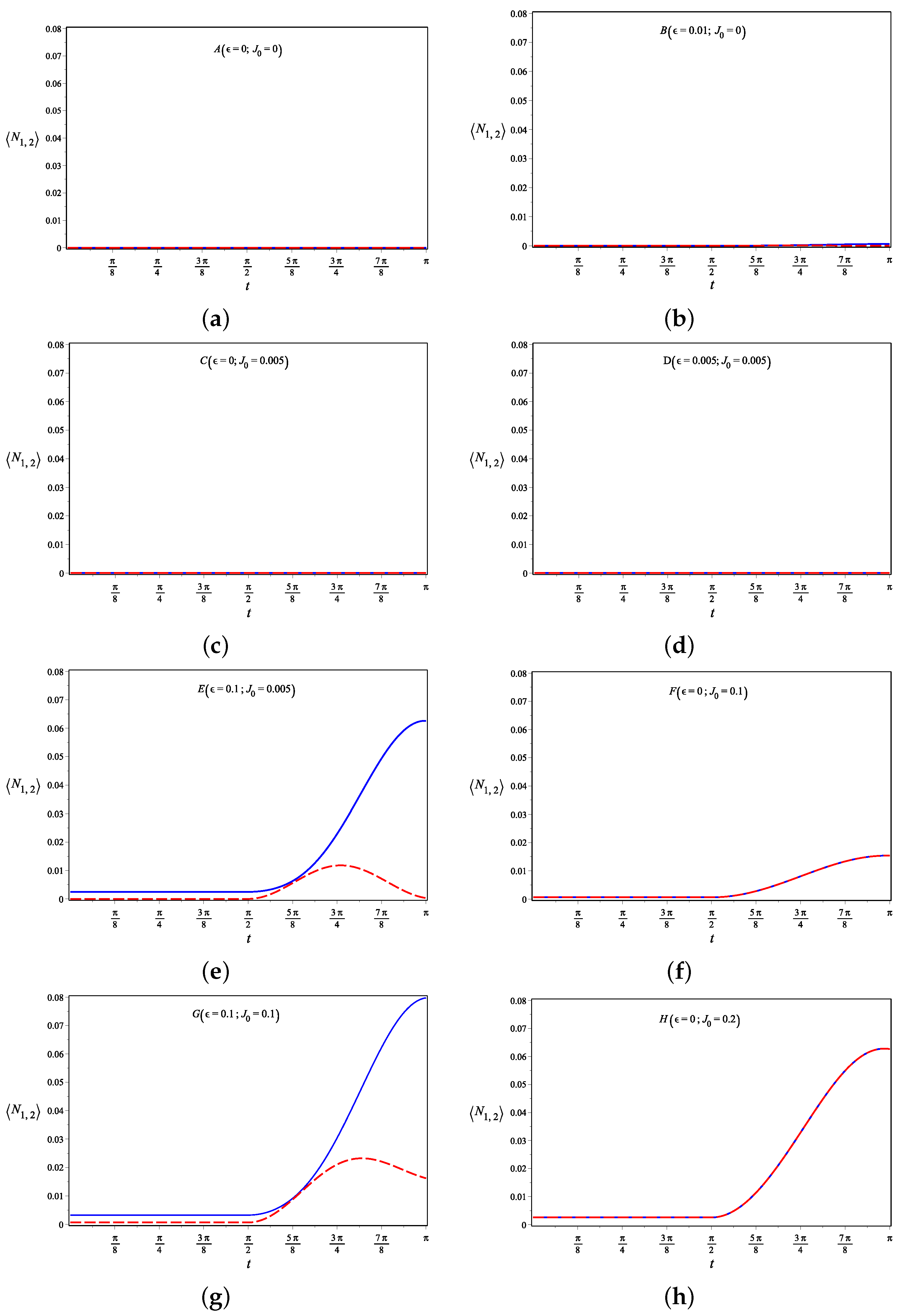
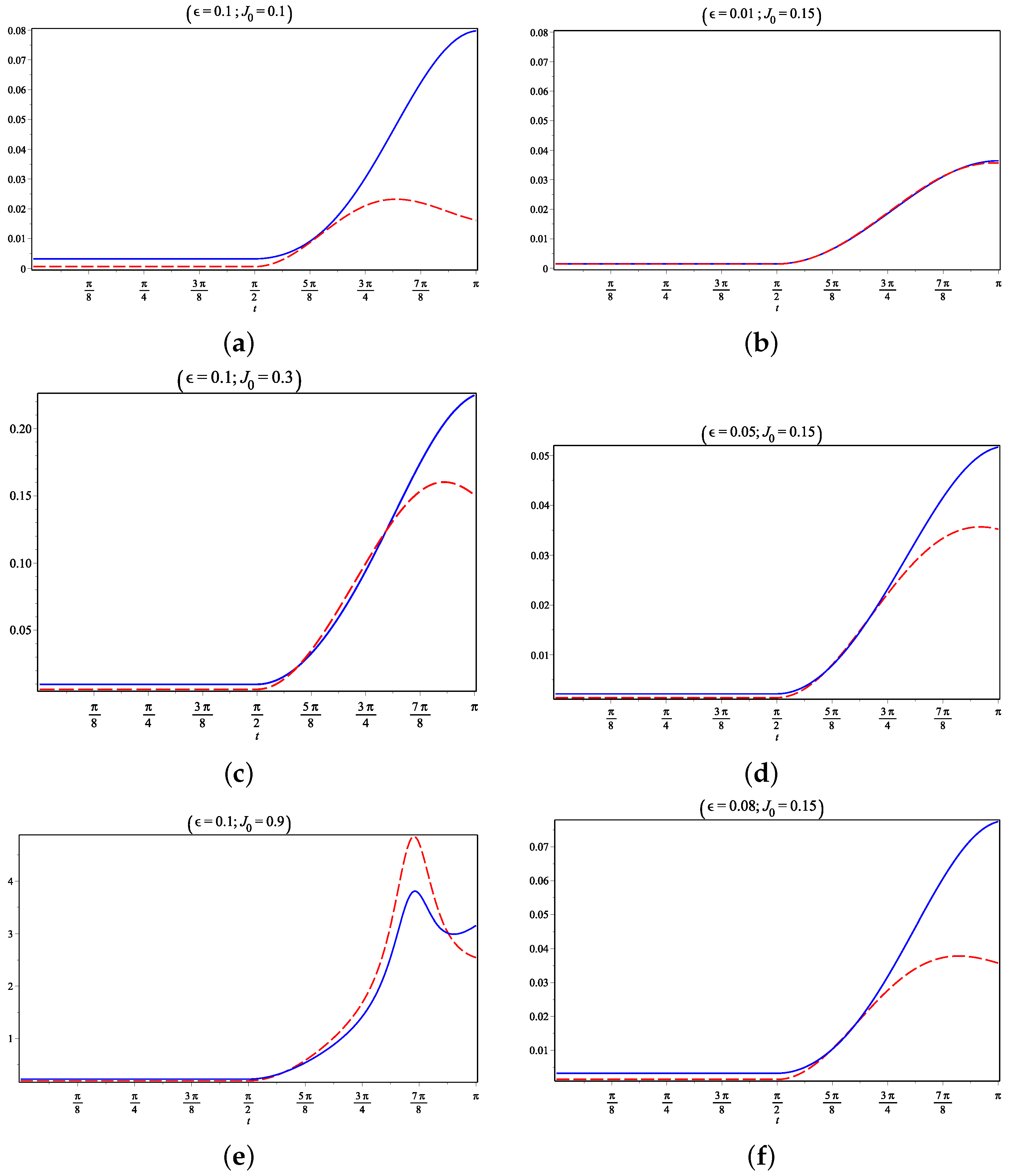
• In the figures of the first column, we set the quench parameter $ϵ$ to $0.1$ and use three values for the coupling, $0.1,0.3$ and $0.9$ from top to bottom. For $J_0=0.1$, excitations in mode 1 exceed those of mode 2 during the entire interval. Then, by increasing the coupling to $0.3$, mode 1 remains initially more populated than mode 2, but immediately after the quench $t_q=\frac{\pi }{2}$ the hierarchy is inverted, and mode 2 becomes more populated up to some point where the hierarchy is inverted again. By further increasing the coupling to $0.9$, the inversion of hierarchy becomes more pronounced until about $t\sim \frac{15\pi }{16}$, where the excitations exhibit an inverse monotony. This phenomenon of hierarchy inversion can be observed as a redistribution of excitations, which becomes more important with the increase in USC coupling.
• In the figures of the second column, we fixed the ultra-strong coupling to $0.15$ and varied the quench factor $ϵ$ between the values $0.01,0.05$ and $0.08$ from top to bottom. For small quench $ϵ=0.01$, the excitations in both modes are close to each other, while by increasing the quench $ϵ$ the excitations became more discernible but without inverted hierarchy.

To conclude, the hierarchy of VE becomes distinguishable by increasing the quench $ϵ$, i.e., when moving away from resonance. The increase in coupling inverts this hierarchy due to the exchange and redistribution of excitations.

6. Conclusions

We have studied a system composed of two non-resonant coupled harmonic oscillators connected with periodically pumped coupling and frequencies with all of these time-dependent parameters modulated by a square wave. We have solved exactly the Schrödinger dynamics, which eventually results in the Ermakov differential equations. After suitable transformations, we have shown that these classical equations actually determine the evolution of the decoupled quantum Hamiltonian. Under the square wave time modulation, the stability study of these differential equations results in Meissner differential equations, and we have derived the condition of instability and the instability maps for them. We have shown with numerical simulations that, in the weak coupling regime and when the classical dynamics is stable, the two coupled quantum modes are empty of VE, but when increasing the coupling until the USC regime, the dynamics become unstable, and the ground state of the system becomes entangled and populated with VE. Additionally, in the USC regime, entanglement and VE exhibit a similar dynamics, which indicates that excitations are necessary to maintain entanglement between the modes. By defining an instability based quantifier, it is possible to identify entanglement and VE in the USC regime. Finally, we showed numerically that the hierarchy of VE becomes distinguishable as we move away from resonance, while it is inverted as the coupling strength is increased because of the exchange and redistribution of excitations. The present work, in addition to its theoretical merit, may be exploited to evaluate the entangling capacity of a quantum system composed by two coupled oscillators by simply examining the stability of a Meissner classical differential equation.

References

1. Einstein, A.; Podolsky, B.; Rosen, N. Can quantum-mechanical description of physical reality be considered complete? Phys. Rev. 1935, 47, 777. [Google Scholar] [CrossRef] [Green Version]
2. Schrödinger, E. Discussion of probability relations between separated systems. Math. Proc. Camb. Philos. Soc. 1935, 31, 555. [Google Scholar] [CrossRef]
3. Figueiredo Roque, T.; Roversi, J.A. Role of instabilities in the survival of quantum correlations. Phys. Rev. A 2013, 88, 032114. [Google Scholar] [CrossRef]
4. Bell, J.S. On the Einstein Podolsky Rosen paradox. Physics 1964, 1, 195. [Google Scholar] [CrossRef] [Green Version]
5. Hofer, S.G.; Wieczorek, W.; Aspelmeyer, M.; Hammerer, K. Quantum entanglement and teleportation in pulsed cavity optomechanics. Phys. Rev. A 2011, 84, 052327. [Google Scholar] [CrossRef] [Green Version]
6. Lin, Q.; He, B. Optomechanical entanglement under pulse drive. Opt. Express 2015, 23, 24497. [Google Scholar] [CrossRef] [Green Version]
7. Jacobs, K.; Wu, R.; Wang, X.; Ashhab, S.; Chen, Q.-M.; Rabitz, H. Fast quantum communication in linear networks. EPL 2016, 114, 40007. [Google Scholar] [CrossRef] [Green Version]
8. Stefanatos, D. Maximising optomechanical entanglement with optimal control. Quantum Sci. Technol. 2017, 2, 014003. [Google Scholar] [CrossRef]
9. Stefanatos, D.; Paspalakis, E. Boosting entanglement between exciton-polaritons with on-off switching of Josephson coupling. Phys. Rev. B 2018, 98, 035303. [Google Scholar] [CrossRef] [Green Version]
10. Stefanatos, D.; Paspalakis, E. Efficient entanglement generation between exciton-polaritons using shortcuts to adiabaticity. Opt. Lett. 2018, 43, 3313. [Google Scholar] [CrossRef] [PubMed] [Green Version]
11. Hedemann, S.R.; Clader, B.D. Optomechanical entanglement of remote microwave cavities. J. Opt. Soc. Am. B. 2018, 35, 2509. [Google Scholar] [CrossRef] [Green Version]
12. Anappara, A.A.; De Liberato, S.; Tredicucci, A.; Ciuti, C.; Biasiol, G.; Sorba, L.; Beltram, F. Signatures of the ultrastrong light-matter coupling regime. Phys. Rev. B 2009, 79, 201303. [Google Scholar] [CrossRef] [Green Version]
13. Frisk Kockum, A.; Miranowicz, A.A.; De Liberato, S.; Savasta, S.; Nori, F. Ultrastrong coupling between light and matter. Nat. Rev. Phys. 2019, 1, 19–40. [Google Scholar] [CrossRef] [Green Version]
14. Gonzalez-Henao, J.C.; Pugliese, E.; Euzzor, S.; Abdalah, S.F.; Meucci, R.; Roversi, J.A. Generation of entanglement in quantum parametric oscillators using phase control. Sci. Rep. 2015, 5, 13152. [Google Scholar] [CrossRef] [Green Version]
15. Gonzalez-Henao, J.C.; Pugliese, E.; Euzzor, S.; Meucci, R.; Roversi, J.A.; Arecchi, F.T. Control of entanglement dynamics in a system of three coupled quantum oscillators. Sci. Rep. 2017, 7, 9957. [Google Scholar] [CrossRef] [Green Version]
16. Chen, R.-X.; Shen, L.-T.; Yang, Z.-B.; Wu, H.-Z. Transition of entanglement dynamics in an oscillator system with weak time-dependent coupling. Phys. Rev. A 2015, 91, 012312. [Google Scholar] [CrossRef]
17. Chakraborty, S.; Sarma, A.K. Entanglement dynamics of two coupled mechanical oscillators in modulated optomechanics. Phys. Rev. A 2018, 97, 022336. [Google Scholar] [CrossRef] [Green Version]
18. Zhou, J.-Y.; Zhou, Y.-H.; Yin, X.-L.; Huang, J.-F.; Liao, J.-Q. Quantum entanglement maintained by virtual excitations in an ultrastrongly-coupled-oscillator system. Sci. Rep. 2020, 10, 12557. [Google Scholar] [CrossRef] [PubMed]
19. Lolli, J.; Baksic, A.; Nagy, D.; Manucharyan, V.E.; Ciuti, C. Ancillary qubit spectroscopy of vacua in cavity and circuit quantum electrodynamics. Phys. Rev. Lett. 2015, 114, 183601. [Google Scholar] [CrossRef] [Green Version]
20. Cirio, M.; Debnath, K.; Lambert, N.; Nori, F. Amplified optomechanical transduction of virtual radiation pressure. Phys. Rev. Lett. 2017, 119, 053601. [Google Scholar] [CrossRef] [Green Version]
21. Zheng, S.-B.; Guo, G.-C. Efficient scheme for two-atom entanglement and quantum information processing in cavity QED. Phys. Rev. Lett. 2000, 85, 2392. [Google Scholar] [CrossRef]
22. Osnaghi, S.; Bertet, P.; Auffeves, A.; Maioli, P.; Brune, M.; Raimond, J.M.; Haroche, S. Coherent control of an atomic collision in a cavity. Phys. Rev. Lett. 2001, 87, 037902. [Google Scholar] [CrossRef] [Green Version]
23. Majer, J.; Chow, J.; Gambetta, J.; Koch, J.; Johnson, B.R.; Schreier, J.A.; Frunzio, L.; Schuster, D.I.; Houck, A.A.; Wallraff, A.; et al. Coupling superconducting qubits via a cavity bus. Nature 2007, 449, 443–447. [Google Scholar] [CrossRef] [PubMed] [Green Version]
24. Ning, W.; Huang, X.-J.; Han, P.-R.; Li, H.; Deng, H.; Yang, Z.-B.; Zhong, Z.-R.; Xia, Y.; Xu, K.; Zheng, D.; et al. Deterministic entanglement swapping in a superconducting circuit. Phys. Rev. Lett. 2019, 123, 060502. [Google Scholar] [CrossRef] [PubMed] [Green Version]
25. Yang, Z.-B.; Han, P.-R.; Huang, X.-J.; Ning, W.; Li, H.; Xu, K.; Zheng, D.; Fan, H.; Zheng, S.-B. Experimental demonstration of entanglement-enabled universal quantum cloning in a circuit. NPJ Quantum Inf. 2021, 7, 44. [Google Scholar] [CrossRef]
26. Pinney, E. The nonlinear differential equation y+p(x)y+cy-3=0. Proc. Am. Math. Soc. 1950, 1, 681. [Google Scholar] [CrossRef]
27. Meissner, E. Ueber Schüttelerscheinungen in Systemen mit periodisch veränderlicher Elastizität. Schweizer Bauzeitung 1918, 72, 95. [Google Scholar]
28. Macedo, D.X.; Guedes, I. Time-dependent coupled harmonic oscillators. J. Math. Phys. 2012, 53, 052101. [Google Scholar] [CrossRef]
29. Moya-Cessa, H.M.; Récamier, J. Comment on “Time-dependent coupled harmonic oscillators” [J. Math. Phys. 53, 052101 (2012)]. J. Math. Phys. 2020, 61, 114101. [Google Scholar] [CrossRef]
30. Menouar, S.; Maamache, M.; Choi, J.R. The time-dependent coupled oscillator model for the motion of a charged particle in the presence of a time-varying magnetic field. Phys. Scr. 2010, 82, 6. [Google Scholar] [CrossRef]
31. Lewis, H.R.; Riesenfeld, W.B. An exact quantum theory of the time-dependent harmonic oscillator and of a charged particle in a time-dependent electromagnetic field. J. Math. Phys. 1969, 10, 1458. [Google Scholar] [CrossRef]
32. Leeach, P.G.L. Invariants and wavefunctions for some time-dependent harmonic oscillator-type Hamiltonians. J. Math. Phys. 1977, 18, 1902. [Google Scholar] [CrossRef]
33. Chen, X.; Ruschhaupt, A.; Schmidt, S.; del Campo, A.; Guéry-Odelin, D.; Muga, J.G. Fast optimal frictionless atom cooling in harmonic traps: Shortcut to adiabaticity. Phys. Rev. Lett. 2010, 104, 063002. [Google Scholar] [CrossRef] [PubMed]
34. Urzúa, A.R.; Ramos-Prieto, I.; Fernández-Guasti, M.; Moya-Cessa, H.M. Solution to the time-dependent coupled harmonic oscillators Hamiltonian with arbitrary interactions. Quantum Rep. 2019, 1, 82–90. [Google Scholar] [CrossRef] [Green Version]
35. Thylwe, K.E.; Korsch, H.J. The Ermakov—Lewis invariants for coupled linear oscillators. J. Phys. A 1998, 31, L279–L285. [Google Scholar] [CrossRef] [Green Version]
36. Richards, J.A. Analysis of Periodically Time-Varying Systems; Springer: Berlin, Germany, 1983. [Google Scholar]
37. Burov, A.A.; Nikonov, V.I. On the nonlinear Meissner equation. Int. J. Non-Linear Mech. 2019, 110, 26. [Google Scholar] [CrossRef]
38. Wang, X.; Vinjanampathy, S.; Strauch, F.W.; Jacobs, K. Ultraefficient cooling of resonators: Beating sideband cooling with quantum control. Phys. Rev. Lett. 2011, 107, 177204. [Google Scholar] [CrossRef] [Green Version]
39. Machnes, S.; Cerrillo, J.; Aspelmeyer, M.; Wieczorek, W.; Plenio, M.B.; Retzker, A. Pulsed laser cooling for cavity optomechanical resonators. Phys. Rev. Lett. 2012, 108, 153601. [Google Scholar] [CrossRef] [Green Version]
40. Franco, C.A.; Collado, J. Comparison on sufficient conditions for the stability of Hill equation: An Arnold’s tongues approach. Appl. Math. 2017, 8, 1481. [Google Scholar] [CrossRef] [Green Version]
41. Tobalina, A.; Torrontegui, E.; Lizuain, I.; Palmero, M.; Muga, J.G. Invariant-based inverse engineering of time-dependent, coupled harmonic oscillators. Phys. Rev. A 2020, 102, 063112. [Google Scholar] [CrossRef]
42. Adesso, G.; Illuminati, F. Gaussian measures of entanglement versus negativities: Ordering of two-mode Gaussian states. Phys. Rev. A 2005, 72, 032334. [Google Scholar] [CrossRef] [Green Version]
43. Adesso, G.; Serafini, A.; Illuminati, F. Multipartite entanglement in three-mode Gaussian states of continuous-variable systems: Quantification, sharing structure, and decoherence. Phys. Rev. A 2006, 73, 032345. [Google Scholar] [CrossRef] [Green Version]
44. Kim, Y.S.; Noz, M.E. Phase Space Picture of Quantum Mechanics; World Scientific: Singapore, 1991. [Google Scholar]
45. Lohe, M.A. Exact time dependence of solutions to the time-dependent Schrödinger equation. J. Phys. A Math. Theor. 2009, 42, 035307. [Google Scholar] [CrossRef]
46. Yeon, K.H.; Kim, H.J.; Um, C.I.; George, T.F.; Pandey, L.N. Wave function in the invariant representation and squeezed-state function of the time-dependent harmonic oscillator. Phys. Rev. A 1994, 50, 1035. [Google Scholar] [CrossRef]
47. Andrews, D.L.; Bradshaw, D.S. The role of virtual photons in nanoscale photonics. Ann. Phys. 2014, 526, 173. [Google Scholar] [CrossRef] [Green Version]
Figure 1. Two coupled oscillators via a position–position type coupling of the form x 1 x 2 . The dynamics generates virtual excitations (VE) that affect quantum quantities.
Quantumrep 03 00043 g001
Figure 2. (a) In the space ( J 0 , ϵ ) and for fixed ω 0 2 = 1 , the points corresponding to bounded Hamiltonian (1) form an open disc of radius ω 0 2 = 1 . (b) Range of parameter points corresponding to bounded Hamiltonian (1) in the space ( J 0 , ω 0 2 ) and for fixed ϵ = 1 .
Quantumrep 03 00043 g002
Figure 3. The stability diagram of Meissner system (20a) and (20b) with modulation (22) in the space ( ϵ , ω 0 ) and for two values of the coupling parameter, (a) J 0 = 0.2 and (b) J 0 = 0 . The upper area corresponds to the unstable region ( S = 0 ) , while the lower area corresponds to the stable region ( S > 0 ) .
Quantumrep 03 00043 g003
Figure 4. (a) Instability region ( S = 0 ) and stability area ( S > 0 ) for the frequency ω 0 2 = 1.01 . (b) Magnification of (a).
Quantumrep 03 00043 g004
Figure 5. The dynamics of VE for fixed ω 0 2 = 1.01 and different values of the quench parameter ϵ and coupling J 0 displayed at the top of the figures. The time dependent frequencies ω 1 , 2 ( t ) of the coupled oscillators are given in Equation (22) and are, thus, determined by the parameters ω 0 , ϵ . The blue solid line corresponds to N 1 , and red dashed line corresponds to N 2 .
Quantumrep 03 00043 g005
Figure 6. For the resonant case ϵ = 0 and fixed ω 0 2 = 1 , we display for three different values of USC coupling J 0 = 0.1 , 0.2 and 0.3 , shown on the top of the figures, (a) the dynamics of entanglement quantified by logarithmic negativity E N and (b) VE N 1 = N 2 = N .
Quantumrep 03 00043 g006
Figure 7. (a) Dynamics of entanglement quantified by logarithmic negativity E N ( t ) and (b) geometric average of excitations M 12 ( t ) = ( N 1 N 2 ) 1 2 , for ϵ = 0.99 , J 0 = 0.01 (blue line) and ϵ = 0.9 , J 0 = 0.1 (red line), while ω 0 2 = 1.01 .
Quantumrep 03 00043 g007
Figure 8. Effect of coupling strength J 0 on entanglement E N ( π 2 ) , geometric average of excitations M 12 = N 1 N 2 1 2 and instability I n s = Λ ( Ω 1 , Ω 2 ) 1 , for (a) ϵ = 0 and (b) ϵ = 0.1 , with ω 0 2 = 1.01 for both cases.
Quantumrep 03 00043 g008
Figure 9. Effects of coupling J 0 (first column) and quench parameter ϵ (second column) on the hierarchy of VE in both modes. The red dashed line corresponds to N 1 ( t ) and the blue solid line to N 2 ( t ) , while ω 0 2 = 1.01 .
Quantumrep 03 00043 g009
Publisher’s Note: MDPI stays neutral with regard to jurisdictional claims in published maps and institutional affiliations.