Abstract
In 1933, Kolmogorov synthesized the basic concepts of probability that were in general use at the time into concepts and deductions from a simple set of axioms that said probability was a -additive function from a boolean algebra of events into [0, 1]. In 1932, von Neumann realized that the use of probability in quantum mechanics required a different concept that he formulated as a -additive function from the closed subspaces of a Hilbert space onto . In 1935, Birkhoff & von Neumann replaced Hilbert space with an algebraic generalization. Today, a slight modification of the Birkhoff-von Neumann generalization is called “quantum logic”. A central problem in the philosophy of probability is the justification of the definition of probability used in a given application. This is usually done by arguing for the rationality of that approach to the situation under consideration. A version of the Dutch book argument given by de Finetti in 1972 is often used to justify the Kolmogorov theory, especially in scientific applications. As von Neumann in 1955 noted, and his criticisms still hold, there is no acceptable foundation for quantum logic. While it is not argued here that a rational approach has been carried out for quantum physics, it is argued that (1) for many important situations found in behavioral science that quantum probability theory is a reasonable choice, and (2) that it has an arguably rational foundation to certain areas of behavioral science, for example, the behavioral paradigm of Between Subjects experiments.
1. Introduction
Quantum logic has been applied in the social sciences, especially in economics and psychology. It has provided insights and alternative explanations to many puzzling behavioral phenomenon. It is a generalization of the logic that is designed to handle quantum phenomena in physics, and it is also a generalization of the classical propositional calculus. It is this second generalization that is the focus of this article, where it is viewed an event space for probability functions with an application to the behavioral science paradigm of Between Subjects experiments.
The following simple example nicely illustrates the properties of quantum logic that apply throughout this article.
Figure 1 is an example of the kind of phenomena and properties of quantum logic that will be used in this article. The Firefly Box is due to Foulis [1]. With a slight change in notation, he writes the following about it:
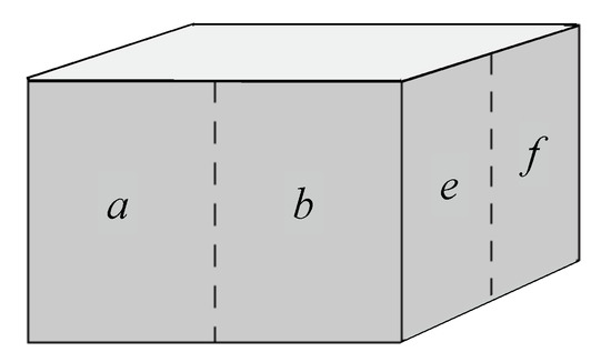
Figure 1.
Firefly Box.
The box is to have two translucent (but not transparent) windows, one on the front and one on the side. The remaining four sides of the box are opaque. At any given moment, the firefly might or might not have its light on. If the light is on, it can be seen as a blip by looking at either of the two windows.
Looking directly at the front window of the box when the light is on, one can tell by the position of the blip whether the firefly is in the left (a) or right (b) half of the box. Likewise, looking directly at the side window when the light is on, one can tell whether the firefly is in the front (e) or back (f) half of the box. Because the windows are not transparent, one cannot rely on depth perception to determine from the front window whether the firefly is in the front or back half of the box, nor from the side window, whether the firefly is in the left or right half of the box.
Now consider two experimental procedures and . Procedure is conducted by looking directly at the front window and recording a, b, or c according to whether the blip is on the left, on the right, or there is no blip, respectively. Procedure is conducted by looking directly at the side window and recording e, f, or d according to whether the blip is in the front, the back, or there is no blip, respectively. One cannot conduct both procedure and at the same time because of the necessity of looking directly at one window or the other. Indeed, if one stands in a position to see both windows, parallax could spoil the accuracy of the observation. (Foulis, 1999).
Let be the combined set of observations, and stand for the power set of X. X generates a boolean algebra of events, . Elements of , called “events”, and are partially ordered by the subset relation, ⊆. Similarly, for let be the boolean algebra of events on , and for , be the boolean algebra of events on .
Repeating procedure provides complete data for the boolean algebra of events ; that is, the experimenter is able to count exactly the number of times each event in has occurred while viewing F, and similarly for procedure . However, this is not the case for the combined structure : There are many events of for which there is no data to account for their occurrence. An example is the intersection of the events and : We can count the number of times a occurs and the number of times f occurs, but not the number of times they jointly occur; is not an observable event. Only observable events have number of occurrences computed from data associated with them. These are called propositions, and their number of (observed) occurrences is exact. Although non-observable events also have a number of occurrences associated with them—after all, they are events occurring in the real Firefly Box world—their numbers are not computable from data; such numbers are said to be “not exact”. A reasonable strategy for theory and data analysis is to only concern oneself with exact probabilities, that is, only concern oneself with propositions.
and have events; all are observable. has events. Because , that is when no light is observed in F, no light is observed S, and vice versa, and thus c and d can be identified. Call this identification k. This restriction reduces the 64 events of to 32. Of these, up to equivalence of membership, 12 are observable. We call them definite events because their members are known and therefore their size can be computed from data.
The event space for probability is generally assume to be a boolean algebra of events, which consists of a set called the sure event, and a nonempty subset of subsets of X such that
- X and the empty set, ⌀, are in ,
- , and
- if A and B are in , then , , and are in , where ∪, ∩, and − are, respectively, set-theoretic union, intersection, and complementation with respect to X.
Elements of are called events, and the empty set, ⌀, is called the impossible or null event. Elements of X are interpreted as possible states of the world, or just states for short. Among the possible states of the world is the true state, which is generally unknown. Associated with is a boolean probability function . For events A in , is interpreted as the degree of belief that the true state of the world is in A. is assumed to have the following properties for all A and B in :
- , , and .
- boolean finite additivity: If , then .
For some applications, a stronger condition than boolean finite additivity is needed:
- boolean σ-additivity: For each countable set of pairwise disjoint events in such that is in ,
This article focuses on the more general case of boolean finite additivity.
1.1. Background: Lattices
The concept of a boolean algebra of events is first generalized to a “lattice algebra of events”, then later specialized to the kind of algebra of events used quantum mechanics, which is here called “quantum logic”. The key idea is to formulate the generalization of ∪ and ∩ in terms of the set-theoretic subset relation, ⊆.
In a boolean algebra of events ∪ and ∩ has the following characterization: For all A and B in ,
- = the ⊆-smallest set C in such that and , and
- = the ⊆-largest set D in such that and .
The above definition of says that C is the ⊆-least upper bound in of A and B and that is the ⊆-greatest lower bound of A and B in . This suggests the following straightforward generalization:
Definition 1.
is said to be a lattice algebra of events if and only if , is a set of subsets of X, and ⋓ and ⋒ are binary operations on such that the following statements hold for all A and B in :
- X and ⌀ are in and .
- is the ⊆-smallest element of such that and .
- is the ⊆-largest element of such that and .
The algebra inherent in boolean algebra of events is captured by the following definition and theorem.
Definition 2.
Let be a lattice algebra of events.
is said to be acomplementation operationon if and only if is a unary operation on such that for all A in ,
is said to be complemented if and only if there exists a complementation operation on .
is said to be distributive if and only if for all A, B, and C in ,
A lattice algebra of events is said to be boolean if and only if it is complemented and distributive. (Note the distinction between a boolean algebra of events and a boolan lattice algebra of events: The boolean algebra has the operations of set theoretic union, ∪, intersection, ∩, and complementation, -, whereas a boolean lattice algebra has the more generally defined operations, ⋓, ⋒, and .
Throughout this article, , where is distributive and is a complementation operation will usually describe a booleanlatticealgebra of events.
Stone [2] showed the following theorem:
Theorem 1.
Each boolean lattice algebra of events is isomorphic to a boolean algebra of events.
Definition 3.
Let be a complemented lattice algebra of events. Then
- is said to satisfyDeMorgan’s Lawsif and only if for all A and B in X,
The following well-known theorem of lattice theory provides an often used alternative formulation of DeMorgan’s Laws.
Theorem 2.
Let be a complemented lattice. Then the following two statements are equivalent:
- (1)
- satisfies DeMorgan’s Laws.
- (2)
- For all A and B in ,
- (i)
- , and
- (ii)
The following is also a well-known theorem:
Theorem 3.
Suppose is a boolean lattice algebra of events. Then satisfies DeMorgan’s Laws.
The lattice literature calls a complementation operation satisfying De Morgan’s Laws an “orthocomplementation operation”, and the special symbol is used to denote it. A lattice algebra of events with an orthocomplementation operation is called an “ortholattice”. Formally, we have the following definitions.
Definition 4.
is said to be an ortholattice with orthocomplementation operation if and only if it is a complemented lattice algebra of events and satisfies De Morgan’s Laws, that is, for all A and B in ,
1.2. Background: Quantum Logic
Theorem 3 below suggests that a complemented lattice satisfying DeMorgan’s laws with a generalization of the distributive law is one natural starting place to find candidates for generalizing boolean event space. For such candidates to be proper generalizations of boolean event spaces, they must be nondistributive. Birkhoff & von Neumann [3] took this approach for their logic for quantum mechanics. Their candidate logic had, in addition to De Morgan’s Laws, is the following generalization implied by distributivity: For all events A, B, and C in the algebra,
Quantum physics is often formulated in terms of Hilbert space. Finite dimensional Hilbert space is an ortholattice of the form, where is the set of subspaces of the Hilbert space, and for A and B in , = the subspace spanned by A and B, and is the operation of orthogonal complementation. (Note the use here of the set-theoretic intersection operation ∩ in the definition of Hilbert Space ortholattice.) For quantum physics, infinite dimensional Hilbert space is sometimes required, and for that case is the set of all closed subspaces. (In the finite dimensional case, all subspaces are closed.) Finite dimensional Hilbert space satisfies the Modular Law. Infinite dimensional Hilbert space requires a weaker law called “orthomodularity”. An ortholattice satisfying orthomodularity is called a “quantum logic”:
Definition 5.
An ortholattice is said to beorthomodularif and only if for all A and B in ,
A lattice is said to be a quantum logic if and only if it is an ortholattice that is orthomodular.
It is well known that distributivity implies modularity and modularity implies orthomodularity.
Quantum logics have a rich algebraic structure that makes some of them interesting candidates for event spaces for probability functions. Many concepts in orthomodular lattice theory are algebraic abstractions of concepts of Hilbert space. One of the most important is “orthogonality”.
Definition 6.
Let be a quantum logic and A and B be in . Then A is said to beorthogonalto B, in symbols, , if and only if .
Definition 7.
Let be lattice algebra of events.
- A in is said to be an atom (of ) if and only if and for all B in , if then or .
- is said to be atomic if and only if for each B in X, if then there exists an atom A of such that .
It is well-known that finite lattices are atomic and that a finite quantum logic satisfies the property that for each of its elements A,
The next section constructs a quantum logic where . The following theorem of Calude, Hertling, and Svozil [4] shows that in general this is permissible:
Theorem 4.
Let be a quantum logic. Then there is an isomorphic quantum logic,
with − as its orthocomplementation operator.
Proof.
Section 2.4 of Calude, Hertling, and Svozil (1999). □
Calude, Hertling, and Svozil (1999) also show similar results for ∪ and ∩:
Theorem 5.
Let be a quantum logic. Then there are isomorphic quantum logics of the form,
and
Thus, one can always choose one of the operations ∪, ∩, − in place of, respectively, ⋓, ⋒, . For example, in modeling quantum physics, ∩ is chosen for ⋒. One cannot model non-distributive quantum logic with ∪ and −, because, by DeMorgan’s Laws, the result would be a distributive logic; similarly for ∩ and −. The quantum logic discussed in the following section chooses − for .
Harding & Pták [5] show the following theorem.
Theorem 6.
Let be a quantum logic and be a boolean lattice subalgebra of . Then there exist a set Y and a mapping φ from X into into the powerset of Y, , such that for all A and B in ,
- ;
- ;
- ;
- .
The following section concerns a social science application of quantum logic. It uses a representation for a quantum logic where . It’s events have probabilities associated with them through relative frequencies, and it is argued in that section that the system of resulting probabilities is coherent, that is, displays rationality. Section 3 also provides concluding remarks.
2. Between Subjects Experiments
Modeling methods inspired by quantum mechanics have recently entered into the social sciences in order to explain many of the context and order effects routinely found in social science experiments. These effects often produce empirically observed failures of boolean finite additivity. This section explores an empirically based theory designed to avoid order and context effects—the popular “Between Subjects paradigm”. The ideas and method generalize to more complicated situations—even ones involving infinitely many experiments, each with infinitely many outcomes. Going from the simple finite case described in this section to more general ones just requires additional technical methods, e.g., Abraham Rorbinson’s “nonstandard analysis”.
The experimental situation considered throughout this article is similar to those in [6,7], except that this article’s definition of a quantum probability function applies to more situations than the orthoprobability functions of Narens (2016 a.b), and changes to notation and proofs have been made to accommodate for this.
The experimental situation considered in this section assumes a large population of subjects and an overall experiment involving six distinct outcomes, . is divided into two sub-experiments, and . A large number of subjects for is assumed, half randomly assigned to and half to . has outcomes, and outcomes . Each subject selects one outcome from her assigned experiment. Attached to subject i, are binary pairs , where and . The interpretation of is that before experiment is performed, subject i will choose x if put in and will choose y if put in .
The collected data about comes from the two sub-experiments. This results that some events A in do not have data that informs the number of times A has occurred. This is because that that information is non-accessible to the observer. For example, data has been collected in that tells how many times the outcome a has occurred, and data in in about how many times the outcome f has occurred, but no data collected about tells many times the joint event has occurred. The joint event is not observable in experiment E. In this article, we take the position that even though the exact number of times has occurred is non-accessible, it did occur some exact number of times. Increasing the number of subjects, does not help in estimating that number.
With slight abuse of notation, we will identify throughout this article the outcome x of an experiment with the event of that experiment.
Convention: Throughout the rest of this section, let S stand for the set of subjects participating in E, stand for those participating in , and stand for those participating in . Let , , , and ,
For each finite set Z, let stand for the number of elements in Z. Let S be the set of subjects participating in experiment . Then, by the way and were chosen,
For each i in S and x and y in X, we say that is the choice set of i if and only if before running experiment , i would choose x if placed in and would choose y if placed in .
For each A in , let
Because S is a large set and X is a small set (i.e., has six elements) and equal numbers of subjects in S were randomly assigned to experiments and , there exists a near one-to-one correspondence between and such that for nearly all individuals i in
That is, for all x in ,
if and i chooses x, then is in and would also have chosen x if placed in instead of ,
and similarly, for all y in ,
if and chooses y, then i is in and i would also have chosen y if placed in instead of ,
In experiment , if x is a choice of i, then x is also a choice of in experiment and vice versa, and similarly for experiment . “Near” is used here to indicate there could be a small error in the one-to-one correspondence that goes to 0 as the relative frequencies go to ∞. For purposes of convenience and exposition, we ignore this error. The correspondence captures the idea that the set of choice behaviors of subjects in and are going to be the same due to the equal and random split of subjects.
For each A in , let be the number of subjects that chose A when experiment was run, and let,
For each B in , let be the number of subjects that chose B when experiment was run, and let,
Furthermore, for each C in , let be the number of subjects that chose C when experiment was run, and let,
Then , , and , are, respectively, boolean probability functions on , , and . Furthermore, because (Equation (3)), restricted to is and restricted to is .
The probability can be computed from data for some events in , e.g., the events , , , , , , but not for others, e.g., event the . Those that it can be computed for are called “propositions”. We will show that set of propositions form a quantum logic. To do this, we introduce the following notation and definitions:
- For each G in , let
- Events A and B are said to be equivalent, in symbols, , if and only if . It easily follows that ≡ is an equivalence relation.
- It is convenient and useful to identify each ≡-equivalent class with its ⊆-largest element. (Such an element exists, because is in and is ’s largest member.)
- For each , let be the ⊆-largest element of the ≡-equivalent class to which G belongs.
- For each , let .
- H is said to be a proposition if and only if
- (i)
- is (exactly) computable from data, and
- (ii)
- .
For each F in such that is (exactly) computable from data, there exists a proposition that is ≡ to F. In some cases different F can have the same proposition equivalent to it. For example, , but - Let P stand for the set of propositions.
This article takes the perspective that is the correct function for describing probabilities on . Although correct, it is somewhat problematic: We know some of its probabilities exactly while others only vaguely with their probabilities somewhere between two exact ones. Furthermore, increasing the number of subjects does not change this, including taking the relative frequency approach to the limit. This suggests restricting the probability function to events with exact probabilities; that is, restricting the probability function to propositions. This article shows that for Between Subjects experiments, a surprising rich theory results: a quantum logic with a probability function that assign to events their relative frequencies. The following describes the steps in achieving this.
First the operations ⋓, ⋒, and ⊥ are defined on P as follows:
Definition 8.
For all propositions F and G inP,
- .
- .
- .
Using these definitions, the following theorem results:
Theorem 7.
is a quantum logic, where is set-theoretic complementation, −, and assigns to propositions in P their relative frequencies, and is additive n P in the sense that
Proof
Lemma A6 of the Appendix A shows is an ortholattice. Thus, to show it is a quantum logic, it needs only to be shown that the orthomodular law holds. Suppose A and B are in P and . We need to show that
Thus, will be done by noting that both and A are propositions and showing,
By the definitions of “⋓” and “⋒”,
Thus, because and ,
is additive because it is a boolean probability function on and, in , for all C and D in P such that ,
and thus that
because C and D are propositions. □
Note that Theorem 7 results from empirical considerations about Between Subjects experiments: All the definitions of the relations making up are empirically based and are computable from the collected data from a Between Subjects experiment.
However, there is more. is also a boolean probability function on
Section 3 argues that this makes a rational assignment of probabilities to P.
Figure 2 diagrams the lattice of propositions for experiment E with outcomes c and d satisfying . It is also a diagram of the lattice of propositions resulting from the firefly example of the Introduction. In the diagram, k is used to replace c and d, because the choices k provide the same information across experiments as c combined with d. (This idea can be used to extend the Between Subjects paradigm to include cases with the experiments having common outcomes.)
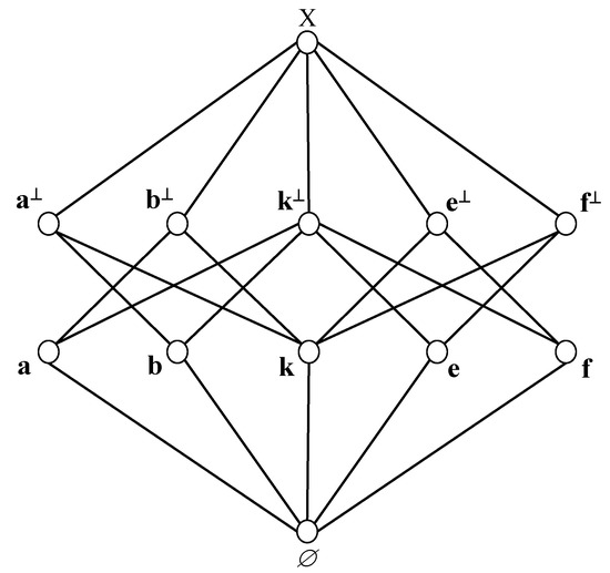
Figure 2.
The lattice of propositions for experiment E (with , k replacing c and d, , and , because of the theoretical assumption c iff d). In this figure, the ⊆ relation is illustrated by moving along a line upward from an open circle (representing a proposition) to another open circle. is the ⊆-largest element of the lattice, ⌀ the ⊆-smallest element, and is an ortho-complementation operation. Boldface letters represent propositions, e.g., a represents the proposition .
Figure 2 is a Hasse diagram of the lattice . The set-theoretic boolean algebra generated by X has elements. The elements at the bottom of Figure 2 are called atoms. They are lattice elements F such that there there does not exist a lattice element G such that . (Note that these atoms of are in boldface because they are not just events; they are propositions, e.g., . Figure 2 has 5 atoms, a, b, k, e, f. These atoms generate a set-theoretic boolean algebra consisting of elements. P has 12 elements—a substantial reduction from 32.
In Figure 2, the lattice-theoretic intersection ⋒ of atoms, e.g., , is the proposition ⌀. However, the set-theoretic intersection of atoms need not be ⌀, e.g., as propositions and , and thus , but is not in the displayed lattice; the largest ⊆-element in the lattice that is displayed as a proper subset of is ⌀.
Busemeyer & Bruza [8] and others have noted that there are many experimental designs in the social sciences that are structurally similar to those in quantum mechanics. Various researchers have taken advantage of this, and have applied methods of quantum mechanics to model social science phenomena. Quantum-like models like these often provide different insights into the mechanisms that generate the experimental data, while often providing equal or better fit to the data.
A criticism of this kind of “quantum mechanical” modeling in the social sciences is that its foundational principles are not adequately justified. For the social sciences, much of fundamental symmetry inherent in quantum physics phenomena is obscure at best and likely does not exist. This is not surprising, because the foundation of quantum mechanics was designed to model the kinds of symmetry found in physical quantum phenomena. An exception appears to be the use of closed subspaces of a Hilbert space as an event space. It applies to many other phenomena. It also provides a simple and useful way to model some dynamic aspects of cognitive phenomena.
3. Concluding Remarks
Heyting algebras, Hilbert space, and quantum logics are three kinds of event spaces that have recently appeared in the literature for modeling probabilistic social science phenomena. They all appear to be useful in providing alternative explanations for unintuitive experimental findings in the cognitive science literature as well providing insights into underlying cognitive mechanisms. All three provide richer mathematical event spaces and probabilistic concepts than boolean probability theory. In psychology, they have been mainly used to explain phenomena where boolean explanations appear inadequate. Although different from one another, the three logics have been used to explain the same troublesome behavioral phenomena.
This article shows that one kind of behavioral science experimental paradigm—Between Subjects experiments—is naturally modeled as a probabilistic quantum logic using concepts derived from collected data. It’s probabilities are empirical relative frequencies.
There has been several results, and some controversy, in the literature concerning the relationship of probability on quantum logics to probability on boolean algebra of events. For the special case of Between Subjects experiments, as treated in this article, the following shows it satisfies the Dutch Book argument for rationality—a standard argument in the literature for the rationality of boolean probability theory.
The Dutch Book Argument [9] revolves around the betting between the Bookie and the Bettor. The Bookie assigns tickets to events from a set of tickets, . For each ticket A in , A has the form, win $1 if A occurs and lose $0 if A does not occur, where A is from the boolean algebra of events,
The bookie sets a price for each . The Bettor can buy from the Bookie or sell to the Bookie any finite number of tickets at the Bookie’s set prices. A Dutch Book is said to be made against the Bookie, if it is possible for the Bettor to buy and sell tickets to the Bookie at the Bookie’s set prices, so that for each state of the world that arises, the Bettor cannot lose money, but for some states of the world she can make a profit. Interpreting prices as probabilities, a probability function on results. The Bookie’s assignment of probabilities is said to be coherent if and only if no Dutch Book can be made against the Bookie. The following well-known theorem due to de Fineti (1972) results: The Bookie’s assignment of probabilities is coherent if and only if they form a boolean probability function for . (Many researchers use the term “rational” in place of “coherent”, because they consider the Theorem to be an argument that shows rationality.)
The proof makes use of the fact in an essential way that is boolean algebra of events. This leaves open the issue of, “What if the underlying event space is not a boolean algebra of events, for example, a quantum logic?” I propose the following generalization of the Dutch Book Argument to handle these cases: For an event space having Y as its states of the world, extend the Bettor’s probability assignments to the boolean algebra of events of all events in in such a way that the extended assignments produce a boolean probability function . Then the Dutch Book Argument applied to and says no Dutch Book can be made. However, if it cannot be made for and , it cannot be made for any subset of and restricted to that subset. That is, the Dutch Book Argument would work for the Bookie’s probability assignments if such extensions could be made. For the Between Subjects experimental paradigm discussed earlier in this article, such extensions exist for the quantum logic and its additive probability function: is a boolean probability function on that is an extension of restricted to the set of propositions. The crux of the argument for rationality is the following: If a rational person assigns ’s probabilities to events in , then the restriction of to any subset of is a rational assignment of probabilities, no matter whether a rational person or the Bookie made them.
Funding
This research received no external funding.
Institutional Review Board Statement
Not applicable.
Informed Consent Statement
Not applicable.
Data Availability Statement
Not applicable.
Conflicts of Interest
The author declare no conflict of interest.
Appendix A. Additional Proofs
Throughout this Appendix, we use definitions and concepts developed earlier in the article. In particular, let , where P is the set of propositions arising from a Between Subjects experiment, is set-theoretic complementation, −, and S, ⋓, ⋒, etc., have their definitions as given earlier.
Lemma A1.
Let D be a proposition. Then
- (1)
- (2)
Proof.
(1) follows from the definitions of “proposition” and .
(2) Let i be an arbitrary subject of S such that there exists y in X such that either or .
Suppose . Then i is not in , i.e., . Because D is a proposition, it has an exact empirical probability. Thus, has an exact empirical probability, because and thus . Thus, is a proposition.
Suppose . Then . Then, because , and . Thus, and , and therefore . □
Lemma A2.
Let D be a proposition. Then is a proposition and is a complementation operation on .
Proof.
By Lemma A1 and , is a proposition. By Lemma A1 and the definitions of ⋓ and ⋒,
and
□
Lemma A3.
⋓ is the ⊆-least upper bound operation on .
Proof.
Let F and G be arbitrary elements of . Then, because
it follows that
and therefore is a proposition. Thus,
and
making an upper bound of F and G. Suppose in is such that
Then
and therefore,
showing that is the least upper bound of F and G. □
Lemma A4.
⋒ is the ⊆-greatest lower bound operation on .
Proof.
Let F and G be arbitrary elements of . Then, because , it follows that
and therefore is a proposition. Thus,
and
making a lower bound of F and G. Suppose H in is such that
Then
and therefore,
showing that is the greatest lower bound of F and G. □
Lemma A5.
is a complemented lattice event algebra.
Proof.
X is clearly the ⊆-largest element of P and ⌀ is clearly the ⊆-smallest element of P.
Because by Lemmas A3 and A4 ⋓ and ⋒ are, respectively, the ⊆-least upper bound and ⊆-greatest lower bound operators on P, is a lattice event algebra, and Lemma A2 shows that is a complementation operation on . □
Lemma A6.
The complemented lattice event algebra satisfies DeMorgan’s Laws.
References
- Foulis, D.J. A Half-Century of Quantum Logic What Have We Learned? In Quantum Structures and the Nature of Reality. Einstein Meets Magritte: An Interdisciplinary Reflection on Science, Nature, Art, Human Action and Society, vol 7; Aerts, D., Pykacz, J., Eds.; Springer: Dordrecht, The Netherlands, 1999. [Google Scholar] [CrossRef]
- Stone, M.H. The theory of representations for boolean algebras. Trans. Am. Math. Soc. 1936, 40, 37–111. [Google Scholar]
- Birkhoff, G.; von Neumann, J. The logic of quantum mechanics. Ann. Math. 1936, 37, 823–843. [Google Scholar] [CrossRef]
- Calude, C.S.; Hertling, P.H.; Svozil, K. Embedding quantum universes in classical ones. Found. Phys. 1999, 29, 349–379. [Google Scholar] [CrossRef]
- Harding, J.; Ptak, P. On the set representation of an orthomodular poset. Colloq. Math. 2001, 89, 233–240. [Google Scholar] [CrossRef]
- Narens, L. Probabilistic frames for non-Boolean phenomena. Philos. Trans. A Math. Phys. Eng. Sci. 2016, 374, 20150105. [Google Scholar] [CrossRef] [PubMed]
- Narens, L. Topological and Orthomodular Modeling of Context in Behavioral Science. Front. Phys. 2017, 5, 4. [Google Scholar] [CrossRef][Green Version]
- Busemeyer, J.R.; Bruza, P.D. Quantum Models of Cognition and Decision; Cambridge University Press: Cambridge, UK, 2012. [Google Scholar]
- De Finetti, B. Probability, Induction and Statistics; Wiley: New York, NY, USA, 1972. [Google Scholar]


Publisher’s Note: MDPI stays neutral with regard to jurisdictional claims in published maps and institutional affiliations. |
© 2021 by the author. Licensee MDPI, Basel, Switzerland. This article is an open access article distributed under the terms and conditions of the Creative Commons Attribution (CC BY) license (https://creativecommons.org/licenses/by/4.0/).