Article

Graph Approach to Quantum Teleportation Dynamics

Department of Optics, Faculty of Physical Sciences, Universidad Complutense de Madrid, Pza. Ciencias 1, Ciudad Universitaria, 28040 Madrid, Spain
*
Author to whom correspondence should be addressed.
Quantum Rep. 2020, 2(3), 352-377; https://doi.org/10.3390/quantum2030025
Submission received: 19 June 2020 / Revised: 6 July 2020 / Accepted: 6 July 2020 / Published: 10 July 2020

Abstract

:
Quantum teleportation plays a key role in modern quantum technologies. Thus, it is of much interest to generate alternative approaches or representations that are aimed at allowing us a better understanding of the physics involved in the process from different perspectives. With this purpose, here an approach based on graph theory is introduced and discussed in the context of some applications. Its main goal is to provide a fully symbolic framework for quantum teleportation from a dynamical viewpoint, which makes explicit at each stage of the process how entanglement and information swap among the qubits involved in it. In order to construct this dynamical perspective, it has been necessary to define some auxiliary elements, namely virtual nodes and edges, as well as an additional notation for nodes describing potential states (against nodes accounting for actual states). With these elements, not only the flow of the process can be followed step by step, but they also allow us to establish a direct correspondence between this graph-based approach and the usual state vector description. To show the suitability and versatility of this graph-based approach, several particular teleportation examples are examined in detail, which include bipartite, tripartite, and tetrapartite maximally entangled states as quantum channels. From the analysis of these cases, a general protocol is devised to describe the sharing of quantum information in presence of maximally entangled multi-qubit system.

1. Introduction

Quantum entanglement is the cornerstone of modern quantum technologies [1]. Within them, quantum teleportation, the capability to transfer the information encoded in the quantum state of a physical system (e.g., an atom or a photon) to another distant physical system, plays an important role, as its remarkable theoretical and experimental development has shown over the last quarter of a century [2]. Because the first protocol introduced by Bennet et al. [3], a number of milestones have paved the way for a solid settlement of the technology based on it. In 1997, the first experimental evidence was demonstrated by transferring a single photon state [4]. These former experiments, where the distance mediating the quantum transfer was of about a few meters, were followed soon afterwards by the first long-distance experiments, involving several kilometers [5]. In this regard, a record was established in 2012, when the experiments were performed between two laboratories separated a distance of 143 km [6], with the purpose to demonstrate the feasibility of the phenomenon at distances of the order of a low Earth orbit and, hence, to implement quantum key distribution protocols at the global level. That record was overcome shortly after by transferring a quantum state between the cities of Delingha and Lijiang, separated by a distance of 1200 km [7], and then with the aid of the Micius satellite [8], setting a new record and also the basis for global communications. Furthermore, there are other important proposals or milestones in recent years regarding quantum teleportation, such as the possibility to transfer internal quantum states between living organisms (e.g., bacteria [9]), the use of this phenomenon to acquire information from the inside of black holes [10], or the experimental realization of quantum teleportation of qutrits [11]. No doubt, these appealing studies directly point towards the development of more sophisticated protocols enabling the teleportation of complex quantum objects.
Nevertheless, the physical essence of the process still remains the same, regardless of the level of complexity and sophistication involved in all those investigations: an entangled pair of particles is used as the resource necessary to transfer the information encoded in a quantum system to another distant system, in a way that somehow remembers the classical momentum transfer in the so-called Newton’s cradle. In this regard, one wonders whether it is possible to find a conceptual description of the process, which might help us to better understand it without making emphasis on the particular physical substrate, as it is usually the case when we consider the standard quantum formulation. This is an idea underlying analogous descriptions of quantum information transfer processes, such as Penrose’s graphical notation [12] or, more recently, Coecke’s quantum picturialism [13], closer to logic. Another route that can be followed is that of topology. Kauffman and Lomonaco, for instance, have developed an approach to account for quantum logic gates and entanglement operators [14,15]. Different topological surfaces have also been used by Mironov [16,17] to deal with the issue of measuring the Von Neumann entropy.
The present work is motivated by the search of an effective pictorial representation for quantum teleportation in dynamical terms, beyond the more standard state vector views, which in the end are more closely connected to particular physical substrates (electrons, photons, vacancies, etc.). Typically, topological descriptions and descriptors are developed within a static framework, just as an operational tool to classify quantum states or to obtain entanglment relations and measures without involving time. Quantum teleportation, on the other hand, inherently involves evolution in time as the information conveyed by a given system is transferred via a quantum channel (and entangled system) somewhere else, even if time-dependence is not explicitly displayed (this happens, for instance, in the former protocol introduced by Bennet et al.). Hence, one wonders whether it is possible to describe this flow, which involves unitary evolution stages with non-unitary measurements by means of a symbolic language, which captures the essence of the full process and, in turn, maintains direct correspondence with the usual state vector description. As it is shown here, this can be done with the aid of graph theory, and introducing some auxiliary elements and notation, which confers the approach with enough flexibility to mimic a dynamical evolution. Moreover, this description is also general enough as to provide protocols when quantum channels consist even of large quantum systems [18]. In this regard, the relational approach introduced here is intended to build a wider and and deeper understanding of quantum dynamical processes involving entanglement, such as quantum teleportation, which might also be easily transferred to other quantum dynamical problems in a rather simple form despite an eventual gradual increment of the level of complexity involved (e.g., a web or lattice of interconnected qubits).
To tackle the issue, a recent work by Quinta and André [19] has provided us the grounds upon which our graph approach has been constructed. In this work, a relational classification system for N-qubit states is provided, which is based on how many entangled subsystems are involved, in a way that is similar to the search of irreducible representations in group theory. By recasting then the quantum state in the form of an N-variable polynomial, they are able to associate an N-component topological link with such a quantum state. Based on this idea, and taking into account the construction of graphs from the corresponding polynomials and links, we have developed an intuitive graph approach to quantum teleportation processes, which include virtual nodes and edges, on the one hand, and additional labeling for nodes to denote potential states (in contrast to the usual actual states), on the other hand. In this regard, this approach goes beyond more standard approaches that are based on links, which lack this relational versatility of graphs, necessary to generate the idea of evolution or flow in time.
The work has been organized, as follows. To be self-contained, some elementary notions from the polynomial and link approach developed by Quinta and André are introduced and discussed in Section 2. In order to get the flavor of the approach and, hence, make more evident the transition to the graph representation, the particular case of a four-qubit state coupled to an auxiliary six-level qudit is analyzed. Subsequently, the graph approach here considered to account for entangled systems is introduced and discussed in Section 3. The application to quantum teleportation is presented in Section 4, first in the case of the standard protocol, and then in the case of teleportation processes involving three and four qubits. From these cases, a general protocol for coupling of a qubit with an N-party entangled state is introduced and discussed. To conclude, a series of final remarks are summarized in Section 5.

2. Polynomials, Links, and Entanglement

According to Quinta and André [19], N-qubit entangled states can be represented by polynomial and topological links, where each constituting qubit is associated with a variable in the polynomial and a ring in the link structure. Consider the operation of partially tracing over a particular qubit in the N-qubit density matrix that describes such a state. Within this representation, this is equivalent to:
(i)
Setting to zero the variable describing the traced qubit in the corresponding polynomial.
(ii)
Removing the ring related to this qubit from the full system topological link.
The resulting polynomial and link thus describe the reduced density matrix for the remaining N 1 qubits. Accordingly, the subsequent sub-polynomials and sub-links that arise after partially tracing with respect to every qubit provide us with valuable information regarding the entanglement that still remains and, therefore, which is going to characterize every reduced subsystem. Thus, it follows that the original polynomial contains all the monomials associated with all possible maximally entangled subsystems, which can be determined by means of the Peres–Horodecki separability criterion [20,21] (see also [22,23]). This is, somehow, analogous to the criterion introduced in [19] to reduce the polynomials under the presence of redundant monomials (simplification rule): a monomial is irrelevant and, therefore, must be neglected if all of its variables are already present in a lower-order sub-polynomial, which corresponds to a maximally entangled state that does not include other variables.
To illustrate the above assertion, consider the case, for instance, of the quantum state | Ψ 34 from [19] (the subscript ‘34’ is just a classifying label, not relevant to the present work, but introduced establishing a better connection to notation used in the literature), which reads as
| Ψ 34 = | 3 1 a b c | 1 d | 0 ν + | 3 1 a b d | 0 c | 1 ν + | 3 1 a c d | 1 b | 2 ν + | 3 1 b c d | 0 a | 3 ν   + | 2 1 a b | 11 c d | 4 ν + | 2 1 c d | 11 a b | 5 ν .
This state describes a system formed by four qubits (a, b, c and d) coupled to an auxiliary six-level qudit ν (specified by | q ν , with q ranging from 0 to 5). Notice that, in turn, this quantum state consists of several tripartite and bipartite entangled sub-states of the class
| N 1 i j k = 1 2 ( | 00 i j k + | 11 i j k ) ,
with i , j , k = a , b , c , d , i.e.,
| 2 1 i j = 1 2 ( | 00 i j + | 11 i j ) ,
| 3 1 i j k = 1 2 ( | 000 i j k + | 111 i j k ) .
Furthermore, there are also factorizable single and bipartite qubits (note that the difference in notation between factorizable states and entangled ones relies on the superscript associated with the latter, which makes reference to the corresponding class specified in [19]). Physically, the quantum state (1) can be interpreted as the result of coupling a four-qubit system with a qudit, such that the latter couples differently depending on how the four qubits are arranged. For instance, the qudit remains in its ground state if the qubits a, b, and c are entangled, while the qubit d remains independent; if the qubits a and b are entangled, and the qubits c and d remain independent, then the qudit ν couples with its fourth excited state; and, so forth.
In order to determine now the amount of entanglement as well as the polynomials and topological rings that are associated with (1), we first determine the corresponding density matrix and we then partially trace over the qudit ν . The resulting 16 × 16 reduced density matrix reads as
ρ ^ a b c d ( Ψ 34 ) = Tr ν [ | Ψ 34 Ψ 34 | ] Ψ 34 | Ψ 34 = | 3 1 a b c | 1 d d 1 | a b c 3 1 | + | 3 1 a b d | 0 c c 0 | a b d 3 1 |   + | 3 1 a c d | 1 b b 1 | a c d 3 1 | + | 3 1 b c d | 0 a a 0 | b c d 3 1 |   + | 2 1 a b | 11 c d c d 11 | a b 2 1 | + | 2 1 c d | 11 a b a b 11 | c d 2 1 | .
After applying the Peres–Horodecki separability criterion for mixed states to this reduced matrix (details on this calculation are provided in Appendix A), only the subsystems (monomials) a b c d , a b c , a b d , a c d , b c d , a b , and c d are shown to be maximally entangled. Consequently, the associated polynomial is
P = a b c + a b d + a c d + b c d + a b + c d ,
which contains all of the above monomials, except the a b c d one, neglected by virtue of the simplification rule mentioned above. On the other hand, the topological link that is associated with the polynomial (6) is readily obtained by cutting and removing the ring corresponding to the qudit ν 
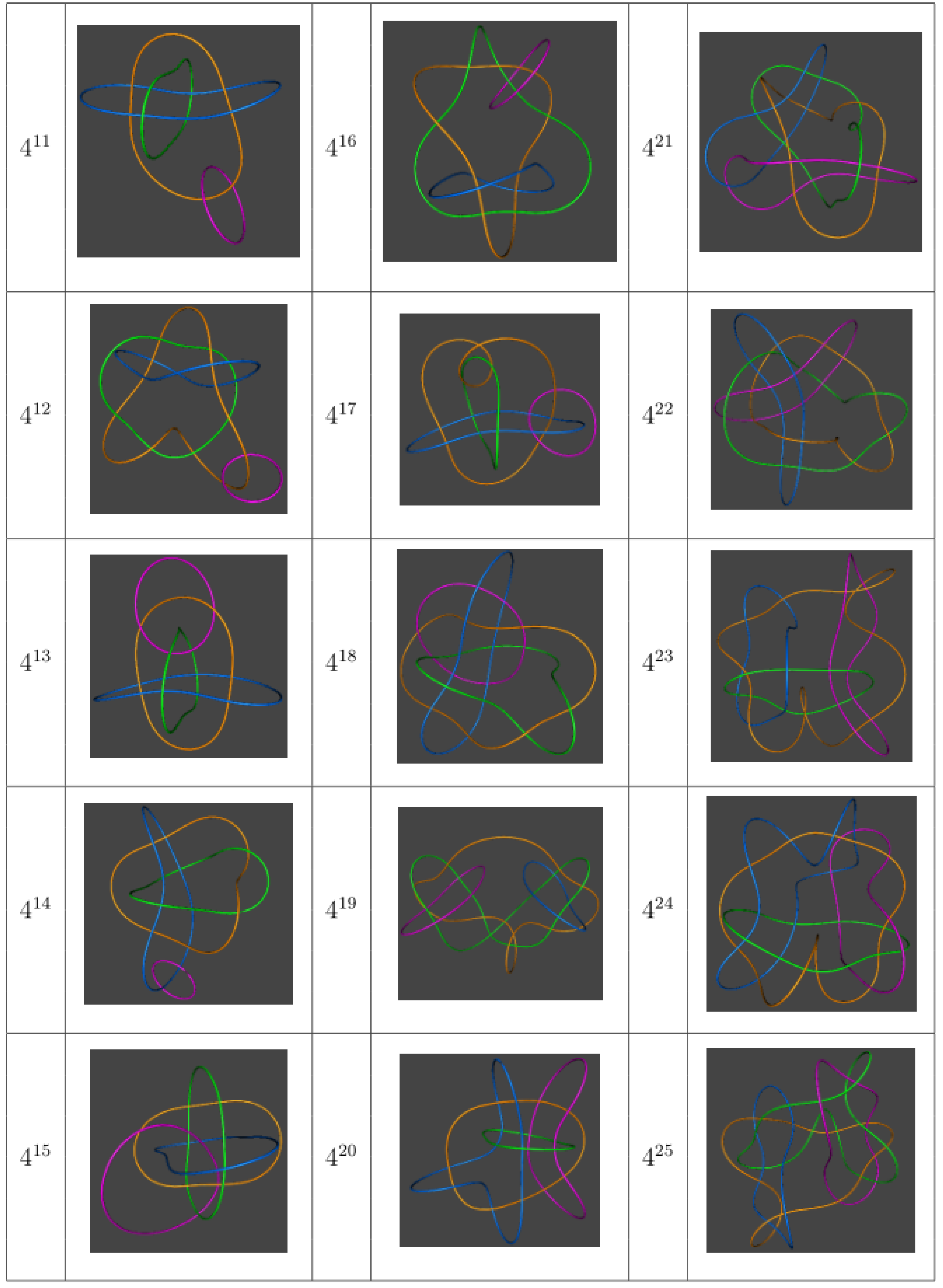
, which is equivalent to setting to zero the associated variable. This process is analogous to chain structures (see, for instance, Figure 11 in [19]), each one representing a monomial with two, three, or four variables. In the particular case of the mixed state (5), the corresponding link representation is displayed in Figure 1, where qubits a, b, c, and d have been denoted with orange, green, blue, and pink rings, respectively, for a better visualization. Furthermore, in order to better appreciate the monomial structure, i.e., the two- and three-variable linking, bipartite entangled structures have been surrounded by yellow and red circles, respectively.
As it can be noticed, a topological description in terms of links is rather convenient to specify entanglement relationships, for it provides us with a general picture of this quantum property without making any explicit reference to a particular physical substrate (material particles, photons, or, in general, different types of degrees of freedom). The key question now is whether the same representation is suitable to describe entanglement transfer or exchange among different quantum systems, which is the case of quantum teleportation. Two drawbacks arise in this regard:
  • The way back is not straightforward, i.e., it is not evident how to generate links that are associated with polynomials from the constituting monomials. This entails difficulties regarding the introduction of some general rules aimed at describing the system splitting after measurement.
  • Although topological links can be useful to elucidate entanglement relationships in systems with a few qubits, the same gets far messier as the number of qubits increases.
At this point, it is clear that we need an alternative representation, which may introduce or describe similar elements, but that, in turn, becomes more versatile, thus providing us with a more suitable framework to deal with the notion of flow of entanglement and information.

3. Graphs and Entanglement

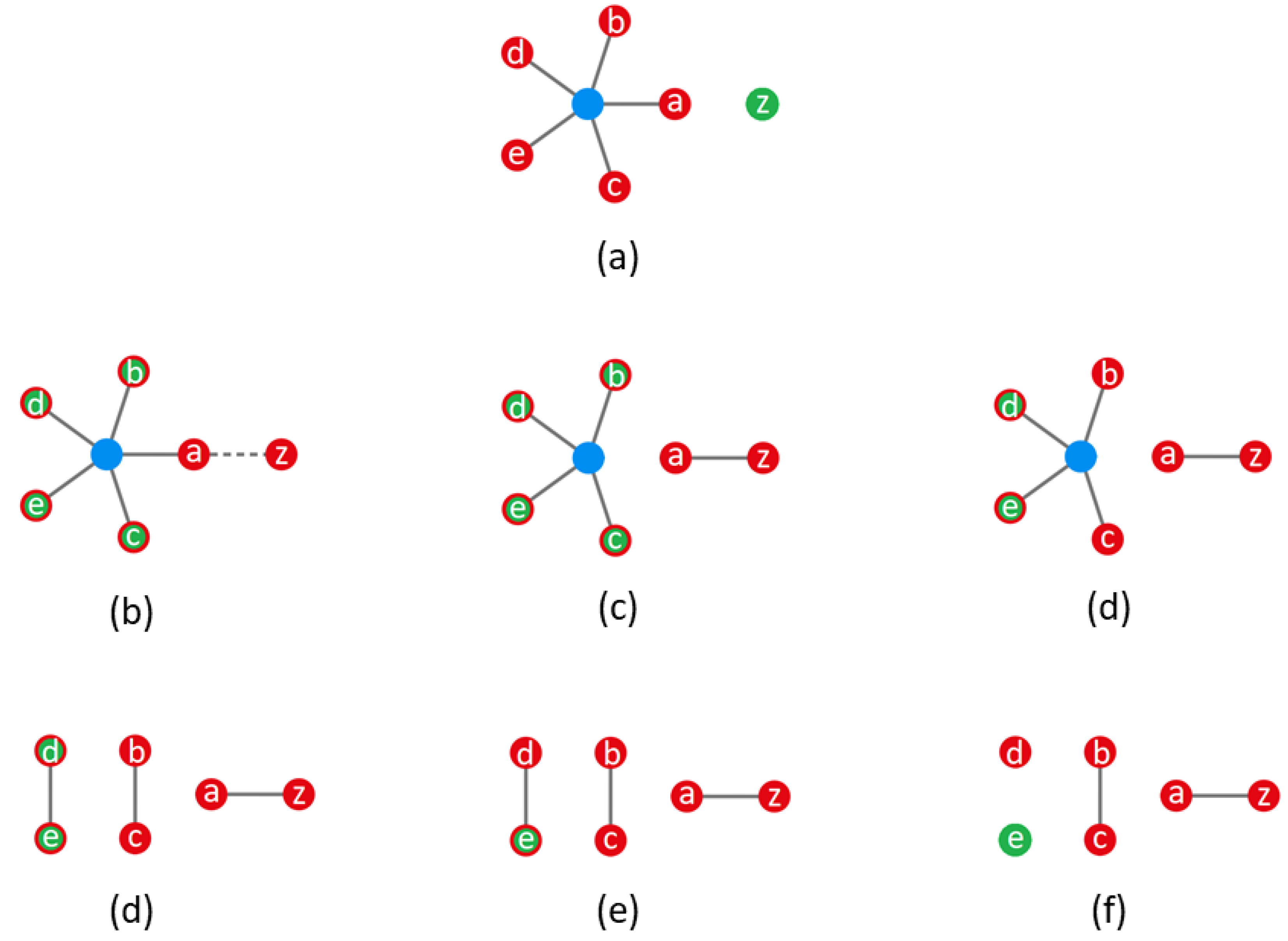
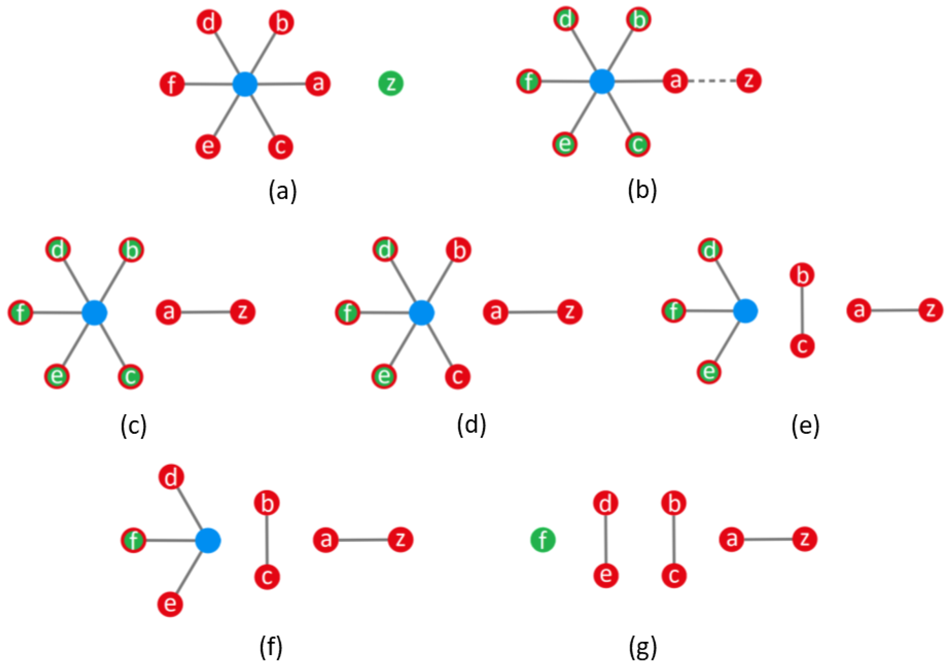
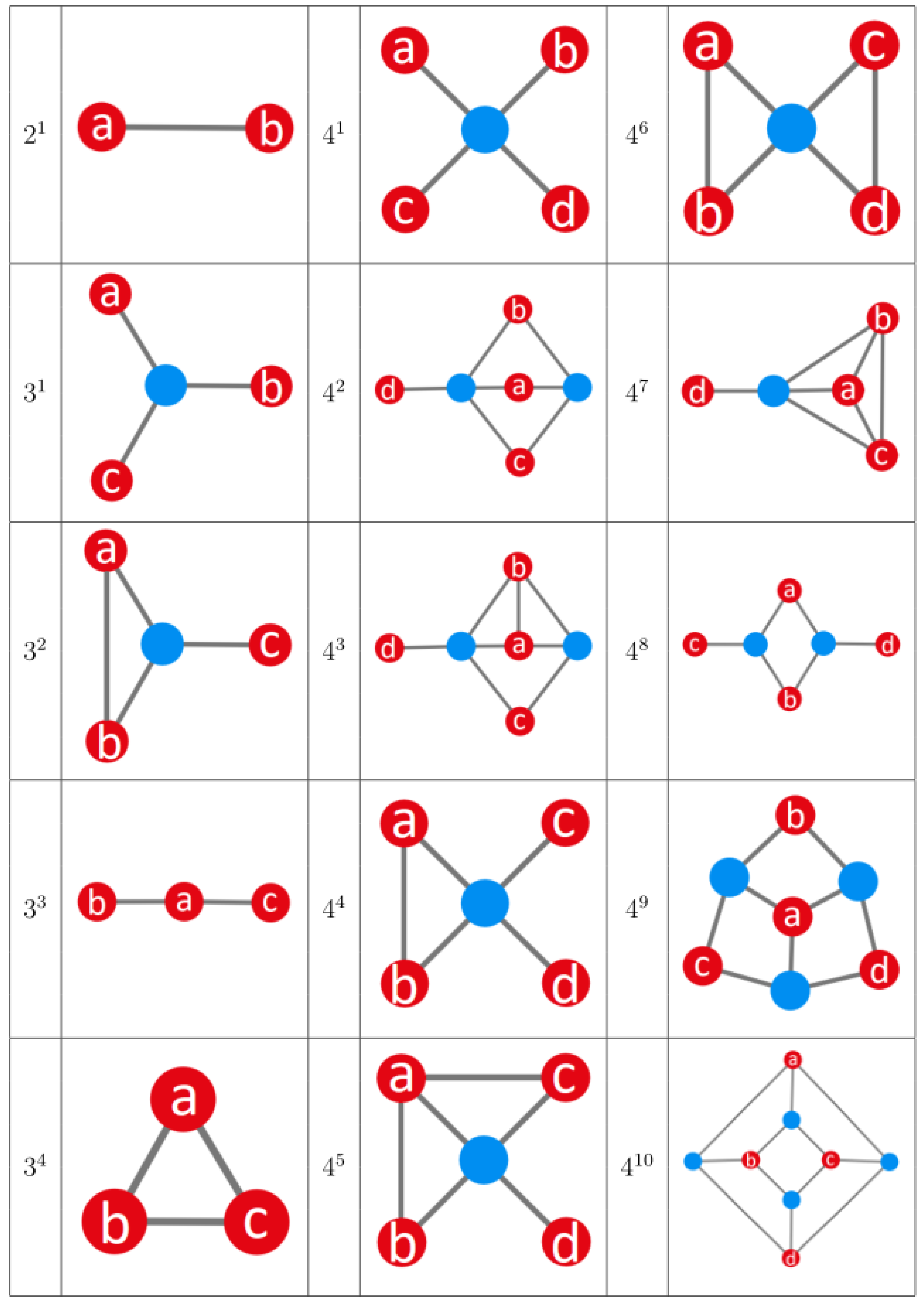
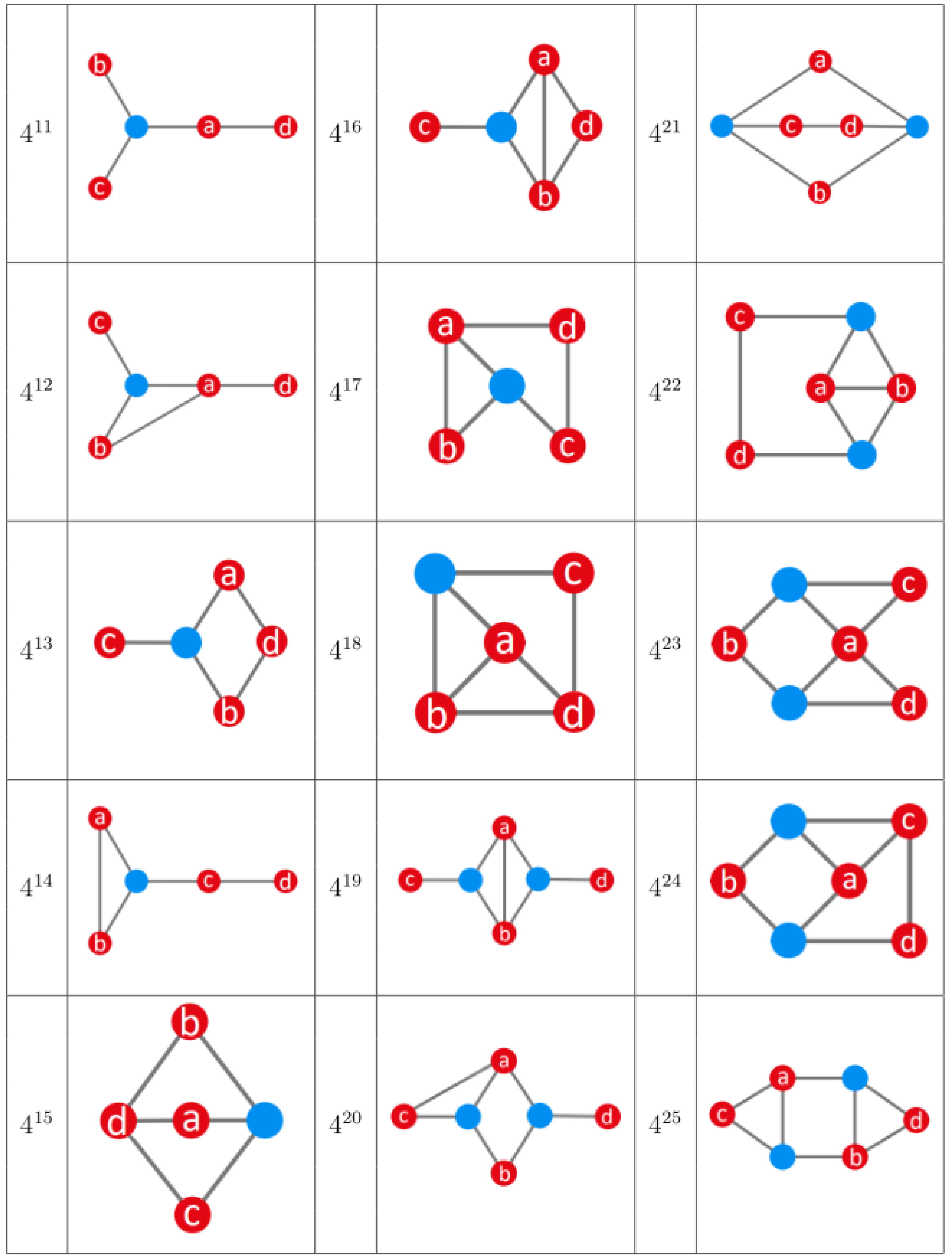
In order to circumvent the above inconveniences, let us thus consider instead a graph representation. In order to move from polynomials to graphs, we associate the variables of a polynomial with (labeled) graph nodes and any entanglement relationship is accounted for by a graph edge. Accordingly, within this scenario, setting to zero a variable is analogous to removing the associated node (and, of course, also the edges incident on it). Now, this is still a rather basic representation, since it only enables a description of polynomials that consist of two-variable monomials; higher-order monomials require an additional level of refinement, for the removal of a node and the corresponding incident edges should not generate a disconnection among the remaining nodes. Notice that this is also necessary, in turn, in order to provide a dynamical view of the entanglement transfer process.
That problem is solved here by defining an auxiliary element in the approach, namely an unlabeled connection or virtual node. Appealing to a color code for simplicity, these virtual nodes are going to be denoted here with blue, while the usual labeled ones will be specified with red. The constructions of graphs by means of these auxiliary virtual nodes follows some simple rules, which also help to simplify the reconstruction of multipartite graphs from elementary ones, just in the same that polynomials are built from elementary monomials. These rules are:
  • Auxiliary nodes are only used to join three or more labeled nodes, which represent entangled states for three or more parties. Accordingly, two (or more) auxiliary nodes cannot be directly connected by an edge.
  • An auxiliary node is redundant if it is connected to three or more labeled nodes chained among themselves by successive edges. Redundant nodes must be removed.
  • If a labeled node is connected to other nodes through a virtual node, the trace over such a node removes not only its edge with the virtual node, but also the latter.
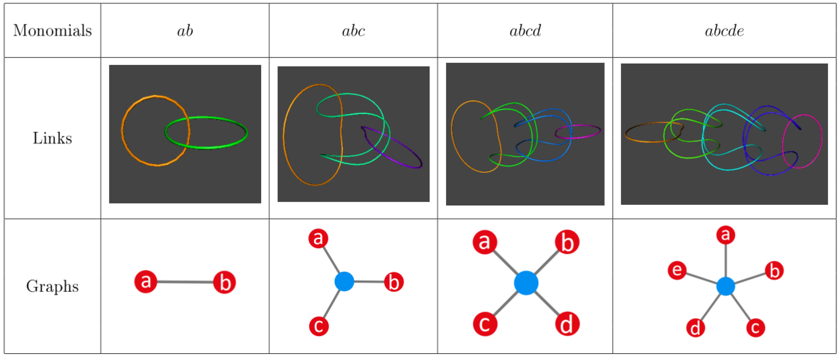
To illustrate the concept, an equivalence table is displayed in 
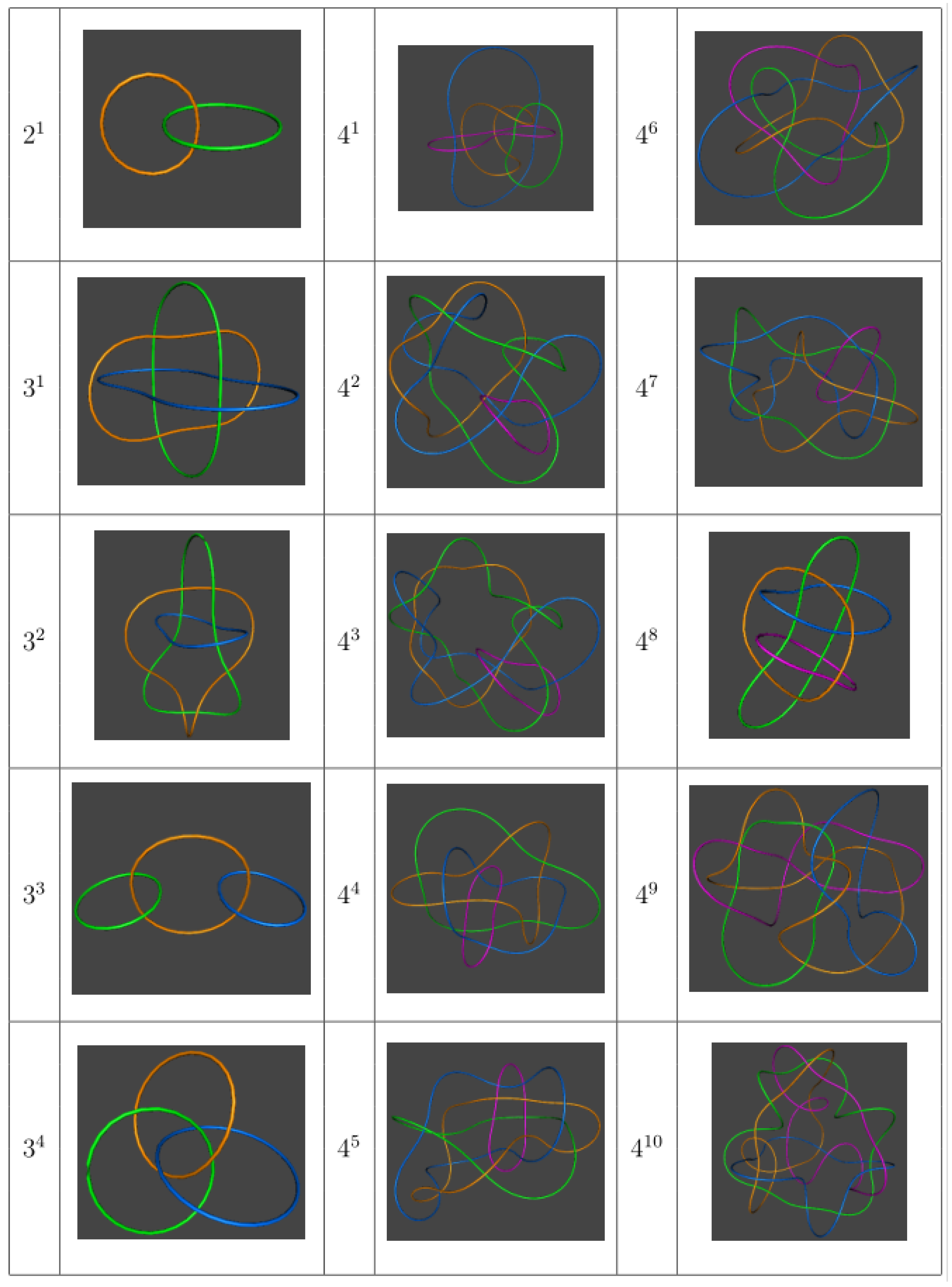
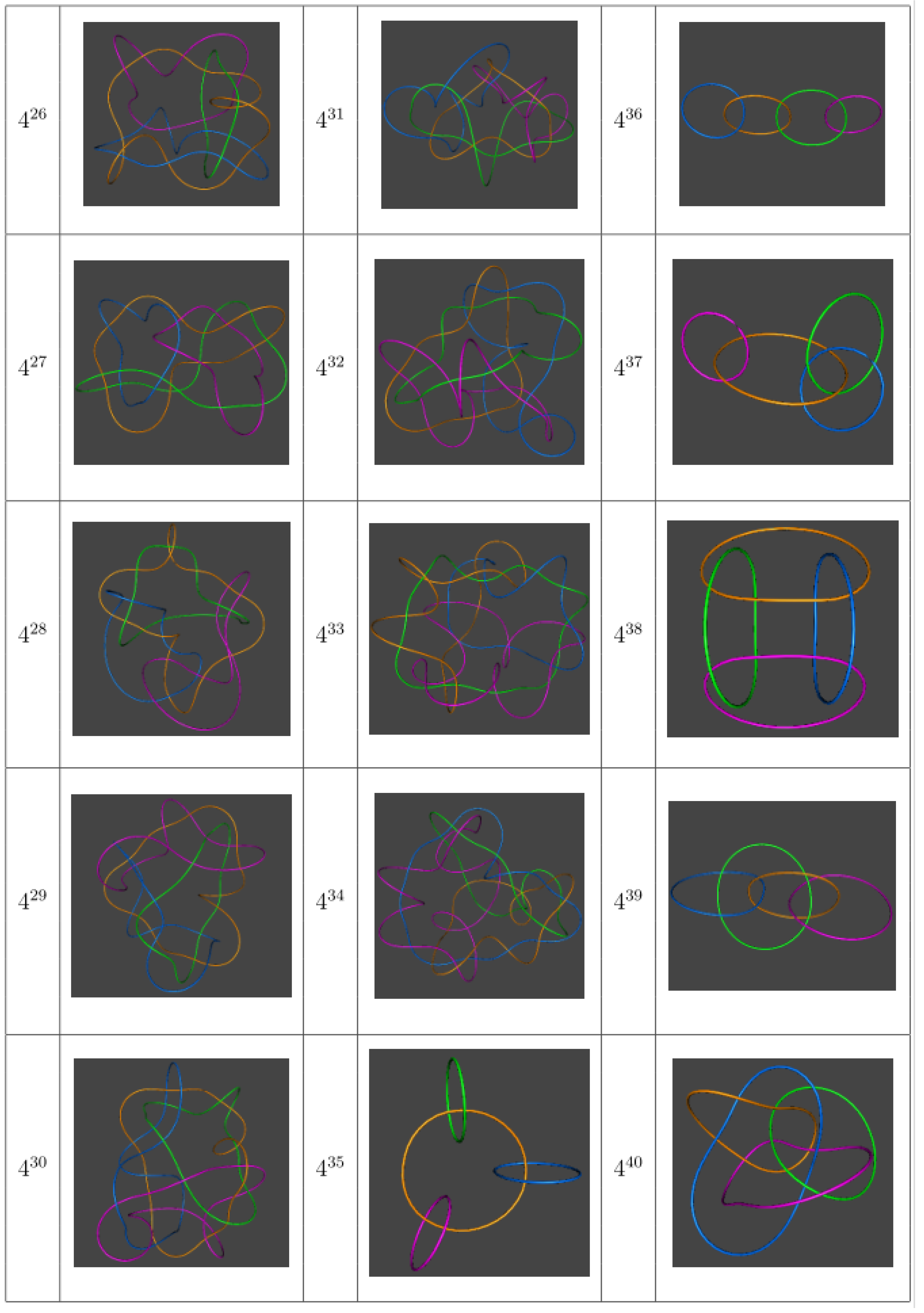
Figure 2, where monomials, links, and graphs for entangled states with a different amount of parties ( N = 2 to 5) are compared. These states have been built following a simple recursive relation with N, which makes more apparent the fact that, when one of the qubits is removed, no matter which one, all other qubits become disentangled immediately. That is, setting to zero a variable completely cancels out the corresponding monomial; cutting a ring, totally releases all other rings. In the case of the graph representation, it can be seen that, for N 3 , the virtual node keeps all qubits entangled. However, as soon as one of such qubits is removed (we partially trace over its states), the virtual node disappears and all other remaining qubits are released. Thus, this approach starts pointing in a direction that seems to favor a description in terms of generation and annihilation of entangled states, which is precisely the case in quantum teleportation, as it will be seen below.
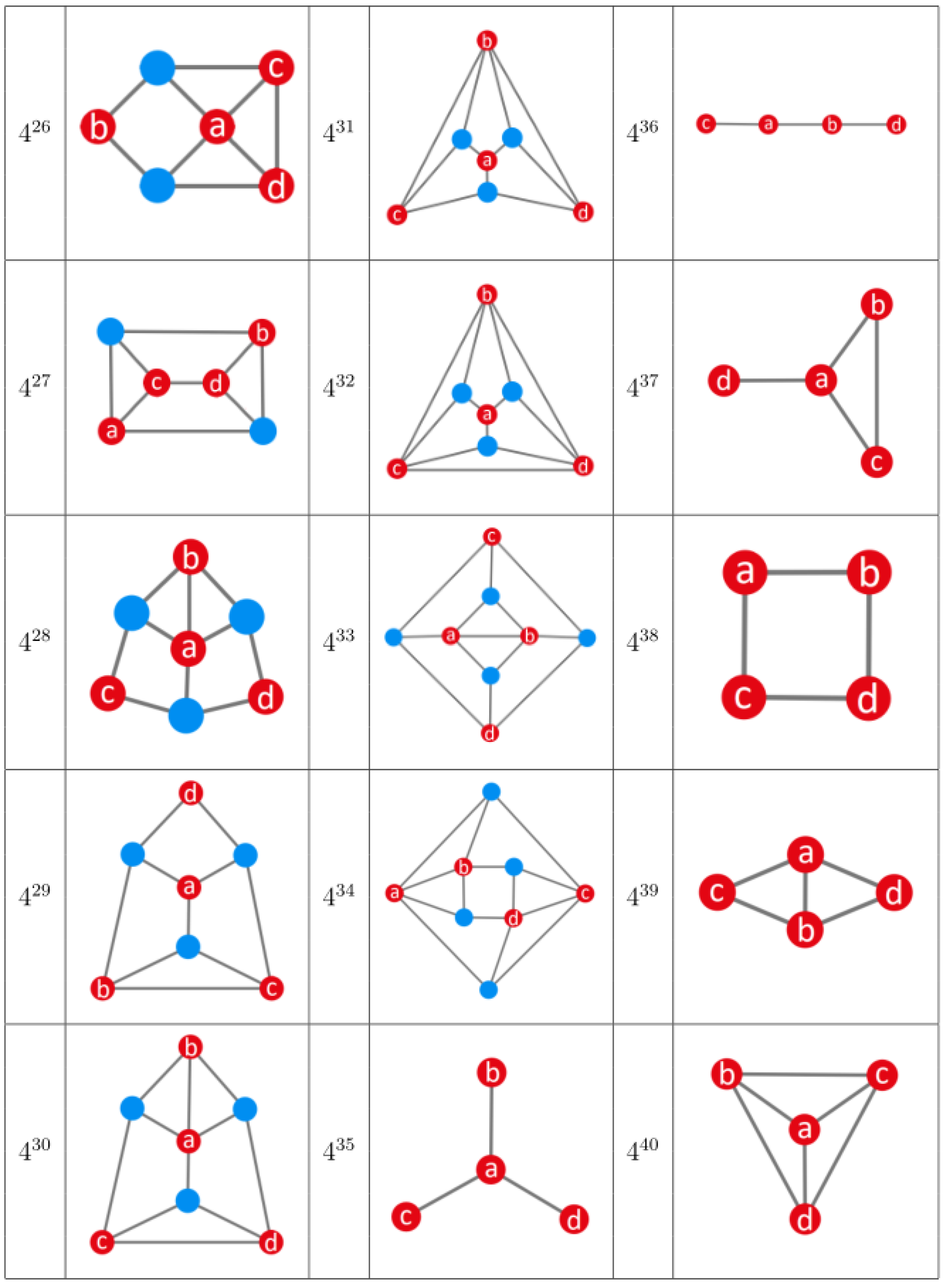
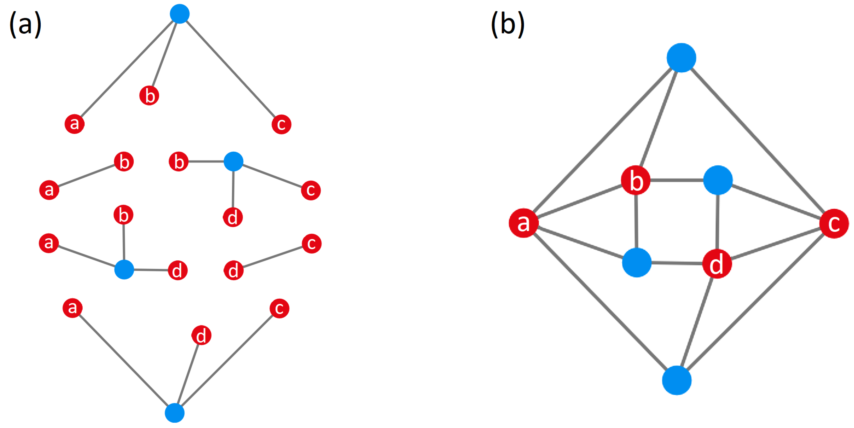
Let us now consider the construction of the graph that is associated with a given polynomial. Without any loss of generality, we are going to consider the polynomial (6). Figure 3a shows the graph representation for the six constituting monomials. These monomials have been arranged in such a way that identical elements (qubits) appear face-to-face, which facilitates the subsequent construction of the final graph. Notice the key role played here, within this arrangement, by the virtual nodes. As it is seen in Figure 3b, these nodes do not disappear when identical elements (labeled nodes) are merged together, because they are not redundant, according to the above rules, rather they provide us a clue on the inverse disconnection process. Furthermore, from this tetrapartite entangled system, the presence of the virtual nodes allows for us to easily identify entangled substructures (monomials) by just following the edges that join them with labeled nodes (for bipartite entangled structures it is enough to follow the edge that joins two neighbor labeled nodes).
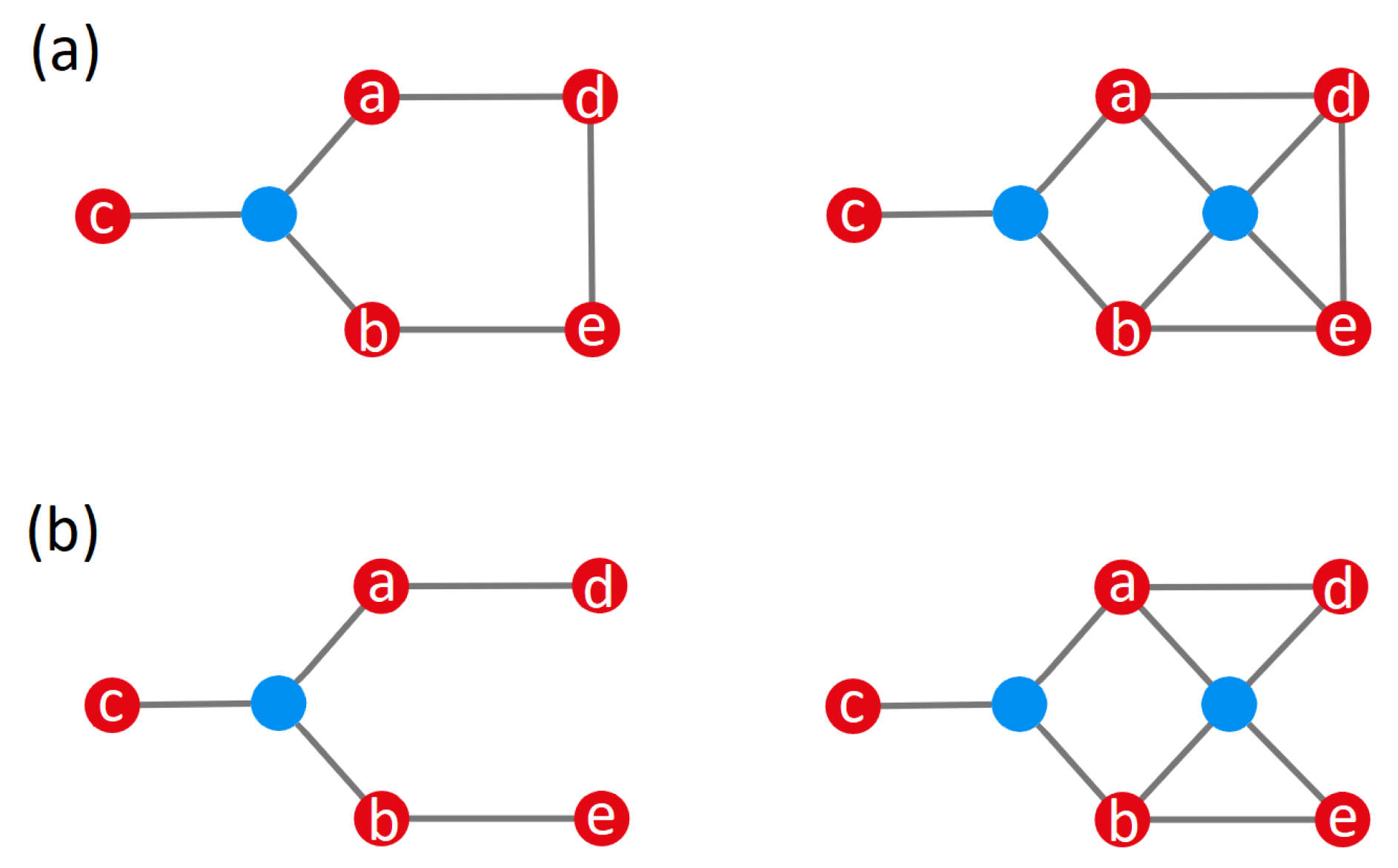
By virtue of the second rule above, graphs can also be simplified. To illustrate this property, consider the pentapartite entangled state described by the polynomial
P = a b c + a d + b e + d e .
The two graphs in Figure 4a are equivalent representations of this polynomial, although the one on the right contains a redundant auxiliary node. Note that this node joins labeled nodes that form a chain, which can be removed without altering the relationship among the constituting qubits, described by the monomials a d , b e and b e . The other virtual node, on the contrary, is not reduntant, describing the tripartite monimial a b c . Now, notice that it is enough removing a single edge, for instance, between d and e, to make such a virtual node not redundant, as illustrated by the two graph representations displayed in Figure 4b. Although they also describe pentapartite entangled systems, these graphs are not equivalent. The graph on the left is associated with the polynomial
P = a b c + a d + b e .
The strategic position of the second virtual node in the graph on the right, on the other hand, additionally contains a tetrapartite entangled subsystem, namely ( a b d e ), thus giving rise to the polynomial
P = a b d e + a b c + a d + b e .

4. Graphs and Quantum Teleportation

In order to determine a proper graph-based description for teleportation processes regardless of the amount of entangled qubits involved in the quantum channel, first we are going to examine several cases, ranging from the typical two-qubit maximally entangled pair to states that include up to five or six entangled qubits. This will provide us with a general set of rules applicable to any case. Nevertheless, in all cases we are analyzing scenarios where the information that is encoded in a given qubit has to be transmitted to a far distant laboratory, which owns one of the parties involved in the corresponding N-qubit entangled state.

4.1. Two-Qubit Entangled State

So far, we have focused on the relational aspects that are involved in entangled states or subsystems. In order to tackle quantum information exchange, as it is the case of quantum teleportation, it is of interest first to briefly see how the process takes place. To this end, let us reconsider the basic quantum teleportation protocol [3], first in the usual state vector representation and then its description in the present graph approach. Accordingly, we have Alice (a), who wishes to teleport the information specified by the quantum state of a qubit (z) that she owns to Bob (b), in a far distant laboratory, by using as a quantum channel the two parties of an entangled pair shared by them. Let us denote the quantum state accounting for the full three-qubit system as
| Ψ z a b = | ϕ z | 2 1 a b ,
which contains the maximally entangled bipartite subsystem a b and the factorized single qubit z. Following the rules provided in the previous section, this state or first stage of the process, can be represented by means of the upper graph displayed in Figure 5a.
After Alice’s entangled party interacts with her qubit, the state describing this new two-qubit system can be recast in terms of Bell-basis vectors as
| Ψ z a b = | Φ z a ( + ) | ϕ b ( 1 ) + | Φ z a ( ) | ϕ b ( 2 ) + | Ψ z a ( + ) | ϕ b ( 3 ) + | Ψ z a ( ) | ϕ b ( 4 ) .
In this second stage, the change of basis is going to induce a series of important modifications in the previous graph structure, as it can be noticed in the middle graph that is shown in Figure 5b, with clear physical implications. First, not only a and z are going to be joined by a virtual (dashed) edge, but z itself is also going to undergo a change in its color in order to make more apparent the new pair a z defined according to the Bell basis set. Moreover, b is also redefined with green color, although surrounded by a red circle, with the purpose to explicitly indicate its potentiality to acquire the information (state) formerly encoded in z. However, the fact that it is still physically attached (entangled) to a, as denoted by then solid edge, is remarked by the red circle.
Therefore, it is only after Alice performs the measurement on her pair of entangled particles, when Bob’s qubit is forced to project over the corresponding Bell vector. By transmission through a classical channel of two bits (operations), Alice communicates to Bob the result of her measurement. Now, he knows the quantum state of his qubit and, by using the correct operator, he finally gets the original state. In terms of graphs, this physical process implies removing the ambiguity of b, which gets physically separated from a (no solid edge between them) and, hence, acquires an unambiguous green color, while a and z become maximally entangled (the virtual edge becomes real). The process is described by the lower graph that is shown in Figure 5c.

4.2. Three-Qubit Entangled State

Using a standard two-qubit entangled state may seem sort of trivial. Let us thus consider a case where three parties share the entangled qubits a three-qubit | 3 1 state, introduced above. The teleportation process for such kind of states is formerly described in [18]. Now, Alice wishes to send the information encoded in | ϕ z to Cliff, but taking into account her partner Bob. Accordingly, the three of them receive in their corresponding laboratories one of the three parties implied in the | 3 1 state. As for the transfer of classical information, unlike the previous setup, this time three bits are required, namely two from Alice to Bob and one from Bob to Cliff. The quantum state describing the four qubits that come into play reads as
| Ψ z a b c = 1 2 cos ( θ / 2 ) ( | 0000 + | 0111 ) + 1 2 sin ( θ / 2 ) e i φ ( | 1000 + | 1111 ) .
The graph representation for this state is provided in Figure 6a, where the physical separation between the a b c entangled system and the z qubit is evident following the description that is provided in Section 4.1. Next, Alice proceeds with a change of basis to describe her qubits z and a, which, in terms of the Bell basis vectors, allows to recast (12) as
| Ψ z a b c = 1 2 | Φ + [ cos ( θ / 2 ) | 00 + sin ( θ / 2 ) e i φ | 11 ] + 1 2 | Φ [ cos ( θ / 2 ) | 00 sin ( θ / 2 ) e i φ | 11 ]   + 1 2 | Ψ + [ sin ( θ / 2 ) e i φ | 00 + cos ( θ / 2 ) | 11 ] + | Ψ [ sin ( θ / 2 ) e i φ | 00 + cos ( θ / 2 ) | 11 ] .
The graph representation for this rewritten state is given by Figure 6b, where the link between qubits a and z is again denoted by the dashed line, while the potential to receive the information encoded in z is denoted by the green labeled nodes encircled by the red (qubits b and c).
Once the tetrapartite state (12) is expressed in terms of the Bell basis set, it is clear that a measurement by Alice on a and z will render any of the four basis vectors with the same probability, releasing the other two qubits, b and c, from their entanglement with a. These vectors become entangled between themselves, being described by a state | 2 1 . This is precisely the situation that is described by the graph displayed in Figure 6c, where the virtual node has disappeared (it is not necessary because we have two separate bipartite entangled states), and the qubits b and c still undefined, as it is denoted by the green-in-red nodes. Remember that, in the case discussed in the previous section, after measurement, the released qubit had already acquired the information initially encoded by z (thus becoming green). Such an undefined state stresses the potential for any of these two qubits to acquire the state of z.
The next step is rather subtle. Without any loss of generality, let us assume that, after measurement, Alice obtains that the system z a is in the state | Φ + . This means that b c are in the entangled state
| Ψ b c = cos ( θ / 2 ) | 00 + e i φ sin ( θ / 2 ) | 11 .
Accordingly, the information encoded in z is shared by b and c, but neither Bob nor Cliff have it yet. As it can be noticed, a measurement on b would not solve the problem, for it would imply that Cliff’s qubit, c, would be either in the state | 0 or in | 1 , with the corresponding probabilities, but we would not recover the initial state | ϕ . Now, in the same way that in order to reach (14) Alice had to consider a change of basis, the same can be done by Bob, not to a Bell basis, but to a basis set rotated by an amount with respect to the { | 0 , | 1 } . Let us denote this new basis set for Bob { | + , | } , which is related to the old one by means of the transformation
| 1 b = cos ω | + b + sin ω | b , | 0 b = sin ω | + b + cos ω | b ,
where ω is the rotation angle, which can be achieved by means of a Stern–Gerlach magnets for entangled charged particles or polarizers for photons (this angle could be taken equal to 45 , for instance). Accordingly, the state for b c can be written as
| Ψ b c = [ sin ω cos ( θ / 2 ) | 0 c + cos ω sin ( θ / 2 ) e i φ | 1 c ] | + b   + [ cos ω cos ( θ / 2 ) | 0 c + sin ω sin ( θ / 2 ) e i φ | 1 c ] | b ,
which is represented by the graph shown in Figure 6d. As it can be noticed in this figure, the ambiguity has disappeared from qubit b; all potentiality relies on qubit c.
The last step thus consists of Bob performing a measurement of his qubit in the new basis, and classically trasmitting the result to Cliff, so that he can then proceed to specify the state of his qubit. Actually, depending on such a result, Cliff should apply one of the following operators. If the outcome is | + b , then he should operate his final state by
O ^ + = ( 1 / cos ω 0 0 1 / sin ω ) ,
while for | b it should be used
O ^ = ( 1 / sin ω 0 0 1 / cos ω ) ,
this being in analogy to the operators needed to recover the transmitted state in the standard two-qubit protocol. With this last operator, qubit c is disambiguated and it acquires the information formerly encoded in qubit z, as denoted by the graph that is represented in Figure 6e.

4.3. Four-Qubit Entangled State

The same procedure that is described in Section 4.3 can be now readily extended to entangled states of the type | N 1 if up to N parties are involved in the sharing of information. To illustrate, let us consider N = 4 , where now the information is going to be conveyed from Alice to Dave, the fourth party, with Bob and Cliff playing the passive role of conveyors. In this case, the total state is described by the combination | ϕ z and | 4 1 , which reads as
| Ψ z a b c d = 1 2 cos ( θ / 2 ) ( | 00000 + | 01111 ) + 1 2 sin ( θ / 2 ) e i φ ( | 10000 + | 11111 ) ,
which is represented by the graph that is plotted in Figure 7a. After Alice performs the change of basis for qubits z and a, this state is rearranged in terms of the Bell basis vectors as
| Ψ z a b c d = 1 2 | Φ + [ cos ( θ / 2 ) | 000 + sin ( θ / 2 ) e i φ | 111 ]   + 1 2 | Φ [ cos ( θ / 2 ) | 000 e i φ sin ( θ / 2 ) | 111 ]   + 1 2 | Ψ + [ sin ( θ / 2 ) e i φ | 000 + cos ( θ / 2 ) | 111 ]   + 1 2 | Ψ [ sin ( θ / 2 ) e i φ | 000 + cos ( θ / 2 ) | 111 ] ,
which is denoted by the graph that is shown in Figure 7b. As before, as soon as the relation between qubits z and a is set by means of the virtual node (physically, through the above basis change), all other nodes acquire the potentiality to receive the information encoded in z, thus changing their color to the undefined green-in-red one.
When Alice performs the measurement of a Bell state, the z a bipartite system becomes physically disentangled from the rest, as shown in Figure 7c. If, for instance, Alice measures | Φ + , the state describing the subsequent entangled b c d tripartite system is
| Ψ b c d = cos ( θ / 2 ) | 000 + sin ( θ / 2 ) e i φ | 111 .
Notice now that we can apply the same rotation recipe used in the previous section, though sequentially, that is, first Bob changes the basis of his qubit and then passes the information onto Cliff, who, in turn, proceeding the same way will allow Dave to obtain in his qubit the information encoded in z. This is an option, of course. However, if it happens that Bob and Cliff are in the same laboratory, there is another option that, in turn, allows for preserving a maximally entangled state, which consists in recasting b c in terms of a Bell basis set, so that (20) can be written as
| Ψ b c d = 1 2 | Φ + [ cos ( θ / 2 ) | 0 + sin ( θ / 2 ) e i φ | 1 ] + 1 2 | Φ [ cos ( θ / 2 ) | 0 sin ( θ / 2 ) e i φ | 1 ] ,
represented by the graph in Figure 7d. However, noticed that, unlike Alice’s former step, now only two Bell vectors are involved, which simplifies the measurement process.
Accordingly, from this point on, the procedure is analogous to the one seen in the previous section, for it is only necessary a measurement by Bob and Cliff, and the transmission of the outcome (two bits) by a classical channel, which will be enough for Dave to obtain the replica of z in his qubit, as shown in Figure 7e. Specifically, if the outcome is | Φ + , it means d has automatically acquired the former state of z; if the outcome is | Φ , the projective operator
( 1 0 0 1 )
must be used before.

4.4. General N-Qubit Entangled States

The cases analyzed in Section 4.2 and Section 4.3 provide us with some insight on a general procedure to dynamically describe quantum teleportation processes that involve N-qubit entangled states as a quantum resource. Two sequential routes have been mentioned. From the analysis of teleportation involving | 3 1 states, we found that after the measurement carried out by Alice, the transfer of information is achieved by simple rotations. This procedure is independent of how many qubits are involved in the quantum channel, which makes possible effective transfers among different laboratories, since each party from the entangled system is allocated in one of them. The other procedure, coming out from the analysis including | 4 1 states, consisted in transferring the information by producing two-party rotations in a reduced Bell basis. This procedure is optimal if qubits can be allocated two by two within the same laboratory, which has the advantage that, after transmission, those two qubits are maximally entangled and they can be used eventually as a quantum resource for further operations. Of course, there can also be hybrid options, where some laboratories receives only one party, while others receive two of them.
In all of this, though, we can find or set a kind of general protocol in terms of a graph representation, which allows for us to better understand the different steps of the process, thus providing us with an insightful dynamical picture. This protocol involves a series of common steps, even if there are some variations. Thus, without any loss of generality, let us consider a simple situation, where we can pair as many as possible two-qubit entangled parties. All of the intermediate steps are going to be the same, regardless of N, but not the last one, which will depend on whether N is odd or even, but this is something that we shall specify in due time. Accordingly, given a quantum channel ascribed to an N-party entangled system, with its quantum state denoted by | N 1 , as given by (2), the graph representation of quantum teleporting the state | ϕ z to any of the N parties includes a series of steps, each one accounting for a specific operation. In order to illustrate these steps, we are going to consider the processes that are illustrated in Figure 8 and Figure 9, where the corresponding teleportation processes involved | 5 1 and | 6 1 states, respectively. Accordingly, we have the following steps:
  • Initial preparation. The graph for the | N 1 state is denoted by N red labeled nodes ( a , b , c , d , e , f , g , ), all of them joined by solid edges with a virtual (blue) node, which represents the entangling correlation. In turn, the state | ϕ z is represented by a green isolated (labeled) node. This is what we observe in Figure 8a and Figure 9a.
  • Initial basis change. Alice prepares her two parties, the one from the | N 1 state (a) and | ϕ z , in a way that, when a Bell measurement is performed on this pair, one of the four Bell states is obtained. This introduces in our graph representation some interesting changes. First, such redefinition gives rise to the appearance of a virtual edge between z and a, and the change of color of the former. This indicates that these two parties are going to become entangled, even though a still remains attached (entangled) to the remaining N 1 parties by virtue of the virtual node. Second, because those other N 1 parties are susceptible to receive the state encoded in z, they are represented with green color, remembering the former representation for z. However, because they still remain entangled among themselves, there is a red circle around them. This stage is shown in Figure 8b and Figure 9b.
  • Alice measurement. As a result of the measurement performed by Alice, the z a system disentangles from the rest. Accordingly, the virtual (dashed) node joining z and a becomes real (solid). The remaining N 1 parties are entangled among themselves, but not maximally due to the information transferred to them. The corresponding | ( N 1 ) 1 state is of the same kind as (2), which readily suggest a description of every two constituting qubits in terms of the reduced Bell basis set { Φ + , Φ } . This is the situation described by the graphs in Figure 8c and Figure 9c.
  • Two-by-two bipartite disentangling. Next, two qubits from the | ( N 1 ) 1 state are grouped and their state is separately described in terms of any of the two vectors of the reduced Bell basis. This implies a change of their color to red, because they are assumed to have lost their potentiality to received the information from z. This situation is represented in Figure 8d, but also in Figure 9d,f. In order to complete the disconnection of these pairs of qubits from the rest, a measurement is performed on the reduced Bell basis; the information is conveyed (by a classical channel) to the receiver of the state encoded in z (in the examples of Figure 8 and Figure 9, this role corresponds to either Emily or Fred, respectively). Such a measurement generates bipartite maximally entangled states (which can be later on used, in turn, as a quantum resource), as it is seen in Figure 8e and Figure 9e,g.
  • Single-qubit measurement (only for odd N). As it can be noticed in Figure 9e, when | N 1 involves an odd number of qubits, after the two-qubit disentangling operations, there are two remaining qubits, one of them being the one of interest (Emily’s one, in this case). This requires, as it was seen in Section 4.2, a simple basis rotation and measurement within such a basis for the residual qubit, represented by the graph shown in Figure 9f.
  • Completion of the transfer (teleportation) process. The outcomes obtained after measuring in the last reduced Bell basis (for even N) or in the rotated basis (for odd N) will be transmitted through a classical channel to either Fred or Emily, who proceeding with the corresponding quantum gate operators on their qubit will finally obtain the state encoded in z, as seen in Figure 8f and Figure 9g.
As it can be noticed, apart from conveying the state encoded in Alice’s qubit z to the far distant qubits of Emily (e) or Fred (f), we end up with ( N 1 ) / 2 or N / 2 , respectively, bipartite maximally entangled states of the type | Φ ± , which can be used later on as quantum resources for other purposes.

5. Final Remarks

In spite of power of the standard algebraic approach of quantum mechanics in the field of quantum information transfer processes, it is equally important to have at hand simpler and visual approaches that emphasize the physics that arre involved in such processes from a quick glance, particularly in those cases where many different relations can be established among a rather large number of intervening parties. In other words, models and descriptions that emphasize the relational aspects of such complex systems are at the same footing, in this regard, as tough algebraic representations, which are more susceptible to hiding the physics that we otherwise we wish to readily see. Just to establish a direct and clear analogy, think of a roadmap that allows for us to quickly see the different roads that join some places with others without involving more quantitative measures (distances, heights, weather conditions, etc.), which is what matters at a first glance (other quantitative details are also important, of course, but on the next level).
In that sense, topological and pictorial representations of quantum entanglement and related processes have received much attention, because they emphasize such relational aspects over more quantitative algebraic ones. Now, it happens that they usually make emphasis on a static description, which is suitable for the classification and description of entangled states, or the performance and visualization of certain quantum logic operations. However, quantum processes, such as teleportation, involve a sort of dynamics where entanglement is swapped from one system or subsystem into another. In order to provide a symbolic representation for these dynamics, here we have introduced a graph representation of the phenomenon. With such a purpose, some additional elements, namely virtual nodes and edges, have had to be defined in order to capture the physical essence that is involved in such swapping process and translate it into proper and well-defined graph connections and disconnections.
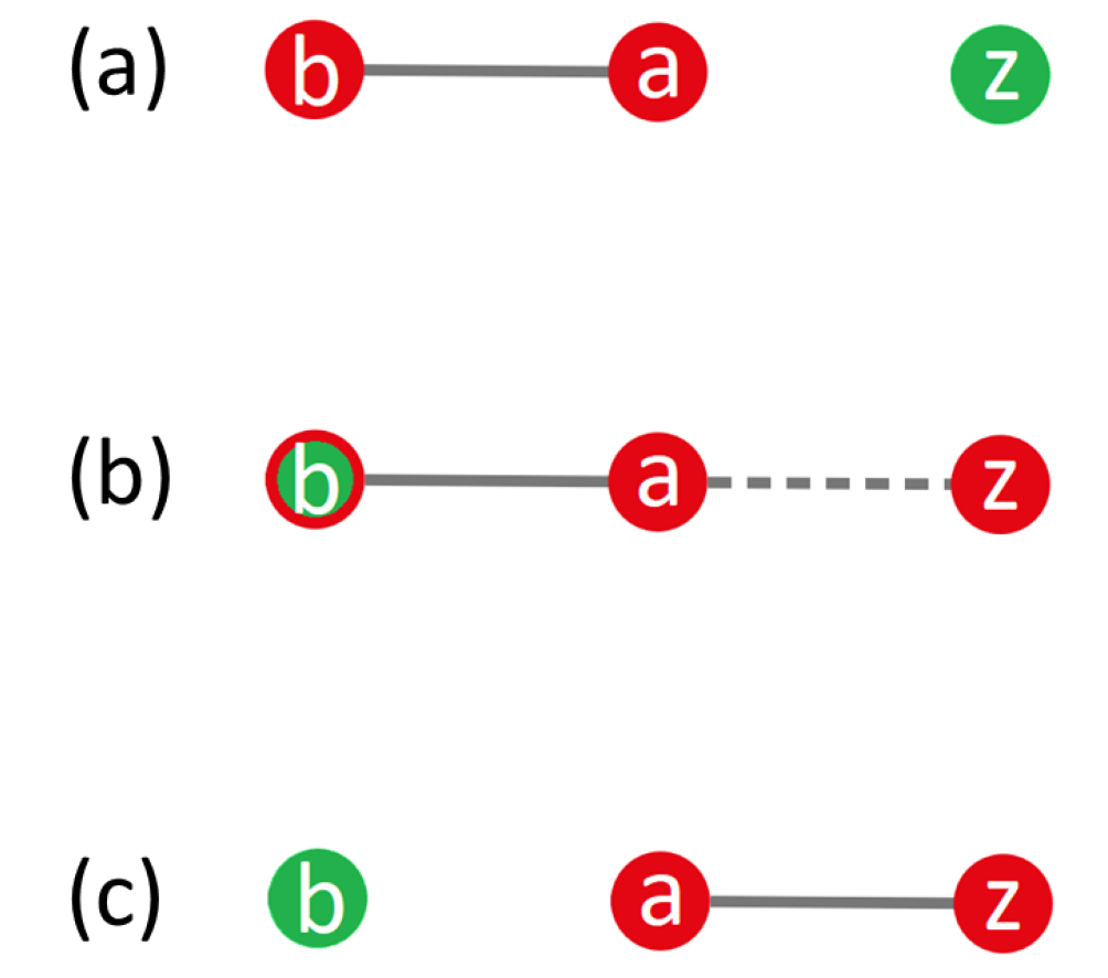
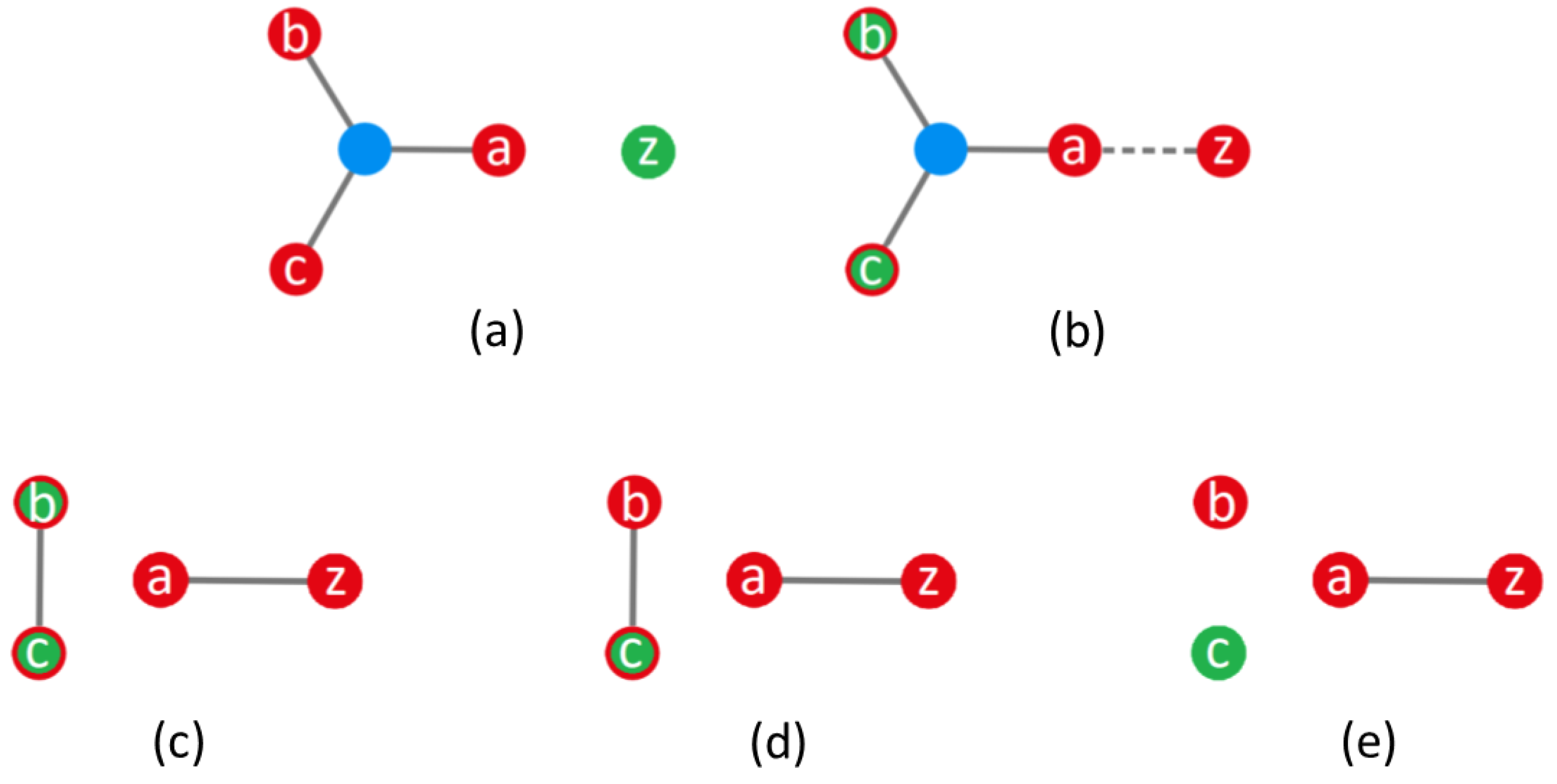
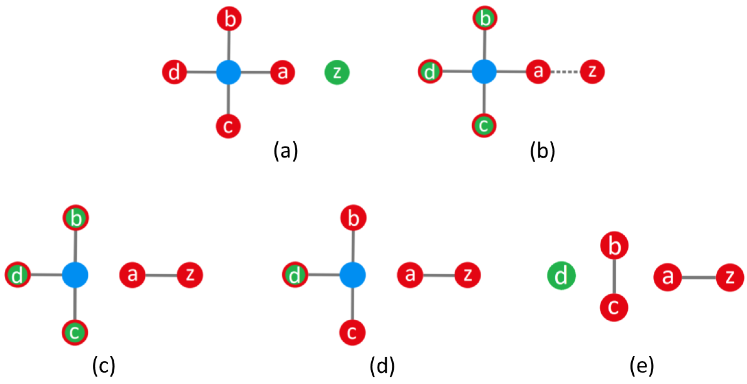
By means of this approach, we have shown that it is possible to reproduce the flow-type evolution involved in quantum teleportation processes, but also to recover at any stage the usual state vector description, because of the one-to-one correspondence between both scenarios, the symbolic and the algebraic. To prove this versatility, we have analyzed and discussed the case of state teleportation while using bipartite, tripartite, and tetrapartite maximally entangled states as quantum channels, and where the corresponding qubits could be accommodated within the same laboratory (by pairs) or in different ones. This has allowed for us to summarize the actions that should be taken in the case of using quantum channels made of any number of qubits with the purpose to share the information available in a given laboratory with any other laboratory forming part of a quantum interconnected network.

Author Contributions

Conceptualization, Á.S.S.; methodology, E.H. and Á.S.S.; software, E.H.; validation, E.H. and Á.S.S.; formal analysis, E.H.; investigation, E.H. and Á.S.S.; writing—original draft preparation, E.H. and Á.S.S.; writing—review and editing, Á.S.S.; visualization, E.H. and Á.S.S.; supervision, Á.S.S.; project administration, Á.S.S.; funding acquisition, Á.S.S. All authors have read and agreed to the published version of the manuscript.

Funding

This research has been funded by the Spanish Agencia Estatal de Investigación (AEI) and the European Regional Development Fund (ERDF) grant number FIS2016-76110-P.

Conflicts of Interest

The authors declare no conflicts of interest.

Appendix A. Entanglement Analysis of the Reduced Density Matrix (5)

The explicit form for the density matrix (5), ρ ^ ( Ψ 34 ) , is given by
ρ ^ a b c d = ( 2 0 0 0 0 0 0 1 0 0 0 0 0 1 0 0 0 1 0 0 0 0 0 0 0 0 0 0 0 0 0 1 0 0 0 0 0 0 0 0 0 0 0 0 0 0 0 0 0 0 0 1 0 0 0 0 0 0 0 0 0 0 0 1 0 0 0 0 1 0 0 0 0 0 0 0 0 0 0 1 0 0 0 0 0 0 0 0 0 0 0 0 0 0 0 0 0 0 0 0 0 0 0 0 0 0 0 0 0 0 0 0 1 0 0 0 0 0 0 1 0 0 0 0 0 0 0 0 0 0 0 0 0 0 0 0 0 0 0 0 0 0 0 0 0 0 0 0 0 0 0 0 0 0 0 0 0 0 0 0 0 0 0 0 0 0 0 0 0 0 0 0 0 0 0 0 0 0 0 0 0 0 0 0 0 0 0 0 0 0 0 0 0 0 0 0 0 0 0 0 0 0 0 0 1 0 0 1 1 0 0 0 0 0 0 0 0 0 0 0 0 1 0 0 0 0 0 0 0 0 0 0 0 0 0 0 0 0 0 0 0 1 0 1 1 0 0 0 0 0 0 0 1 0 0 4 ) ,
where we have removed the normalizing prefactor 1 / 12 without loss of generality, since here we are only interested in the sign of the eigenvalues. So, after computing all the associated partial transpose matrices in order to determine the amount of entanglement, we obtain the following sets of eigenvalues for each one:
ρ ^ a b c d T a ,   ρ ^ a b c d T c :   { λ 1 =   0   ( × 5 ) λ 2 = 1 λ 3 =   1   ( × 5 ) λ 4 =   3 λ 5 1.306 λ 6   0.473 λ 7   1.492 λ 8   4.341 , ρ ^ a b c d T b ,   ρ ^ a b c d T d :   { λ 1   =   0   ( × 5 ) λ 2   =   1   ( × 2 ) λ 3   =   2 λ 4   1.247 λ 5   0.887 λ 6     0.45 λ 7     0.485 λ 8     0.733 λ 9     1.802 λ 10   2.069 λ 11   4.600 ,
ρ ^ a b c d T a b :   { λ 1 =   0   ( × 8 ) λ 2 =   1   ( × 2 ) λ 3 =   2   ( × 2 ) λ 4 0.414 λ 5   2.414 λ 6 0.646 λ 7   4.646 , ρ ^ a b c d T a c :   { λ 1   =   0   ( × 4 ) λ 2   =   1   ( × 4 ) λ 3   =   2 λ 4   =   4 λ 5   0.618 λ 6     1.618 λ 7   2.090 λ 8   0.356 λ 9     1.190 λ 10   2.256 , ρ ^ a b c d T a d :   { λ 1 =   0   ( × 4 ) λ 2 =   1   ( × 2 ) λ 3 =   2 λ 4 =   4 λ 5 1.194   ( × 2 ) λ 6 0.295   ( × 2 ) λ 7   1.295   ( × 2 ) λ 8   2.194   ( × 2 ) .
As it is seen, all cases contain negative eigenvalues, which ensures the existence of entanglement, although now we have to determine whether it is tripartite, bipartite or both, and, if so, which parties are involved.
To proceed that way, first we have to compute the reduced matrices with respect to one of the parties. Thus, partially tracing over d renders
ρ ˜ ^ a b c = ( 3 0 0 0 0 0 0 1 0 1 0 0 0 0 0 1 0 0 1 0 0 0 0 0 0 0 0 1 0 0 0 0 0 0 0 0 0 0 0 0 0 0 0 0 0 0 0 0 0 0 0 0 0 0 2 0 1 1 0 0 0 0 0 4 )
with eigenvalues:
ρ ˜ ^ a b c T a ,   ρ ˜ ^ a b c T b :   { λ 1 =   0 λ 2 = 1 λ 3 =   1   ( × 2 ) λ 4 =   2   ( × 2 ) λ 5 =   3 λ 6 =   4 , ρ ˜ ^ a b c T c :   { λ 1 = 0   ( × 2 ) λ 2 = 1   ( × 2 ) λ 3 = 3 λ 4 0.186 λ 5 2.471 λ 6 4.343 .
Now, not all cases present negative eigenvalues, which means that tripartite entanglement is not warranted for the a b c system. Accordingly, we compute the eigenvalues of (A2):
{ λ 1 = 0   ( × 2 ) { | v 1 , 1 = | 100 | v 1 , 2 = | 101 λ 2 = 1   ( × 2 ) { | v 2 , 1 = | 010 | v 2 , 2 = | 011 λ 3 = 2 | v 3 = | 110 λ 4 0.657 | v 4 = 0.427 | 000 2.916 | 001 + | 111 λ 5 2.529 | v 5 = 2.125 | 000 + 0.654 | 001 + | 111 λ 6 4.814 | v 6 = 0.551 | 000 0.262 | 001 + | 111 .
here, we observe that there are at least three non-factorizable eigenvectors, which ensures the existence of tripartite entanglement for the a b c system.
If now we trace (A1) over the qubit c, we obtain the reduced matrix
ρ ˜ ^ a b d = ( 2 0 0 0 0 0 0 1 0 2 0 0 0 0 0 1 0 0 1 0 0 0 0 0 0 0 0 1 0 0 0 0 0 0 0 0 0 0 0 0 0 0 0 0 0 0 0 0 0 0 0 0 0 0 1 0 1 1 0 0 0 0 0 5 ) ,
with the eigenvalues of its associated partial transpose matrices being
ρ ˜ ^ a b d T a ,   ρ ˜ ^ a b d T b :   { λ 1 =   0 λ 2 = 1 λ 3 =   1   ( × 2 ) λ 4 =   2   ( × 3 ) λ 5 =   5 , ρ ˜ ^ a b d T d :   { λ 1 = 0   ( × 2 ) λ 2 = 1   ( × 2 ) λ 3 = 2 λ 4 0.319 λ 5 2.358 λ 6 5.323 .
Again, one partial transpose has all its eigenvalues positive, so we need to compute the eigenvectors,
{ λ 1 = 0   ( × 2 ) { | v 1 , 1 = | 100 | v 1 , 2 = | 101 λ 2 = 1   ( × 3 ) { | v 2 , 1 = | 010 | v 2 , 2 = | 011 | v 2 , 3 = | 110 λ 3 = 2 | v 3 = | 000 | 001 λ 4 1.438 | v 4 = | 000 + | 001 0.562 | 111 λ 5 5.562 | v 5 = | 000 + | 001 + 3.562 | 111 ,
which contains three entangled eigenvectors and, therefore, ensures tripartite entanglement for the a b d system.
The same trend is found when we proceed with the partial trace over b, which renders the reduced density matrix
ρ ^ a c d = ( 3 0 0 0 0 0 0 1 0 1 0 0 0 0 0 0 0 0 0 0 0 0 0 0 0 0 0 2 0 0 0 0 0 0 0 0 1 0 0 1 0 0 0 0 0 1 0 0 0 0 0 0 0 0 0 0 1 0 0 0 1 0 0 4 ) ,
with eigenvalues for its transposes being
ρ ˜ ^ a c d T a :   { λ 1 = 0   ( × 2 ) λ 2 = 1   ( × 2 ) λ 3 = 3 λ 4 0.186 λ 5 2.471 λ 6 4.343 , ρ ˜ ^ a c d T c ,   ρ ˜ ^ a c d T d :   { λ 1 =   0 λ 2 = 1 λ 3 =   1   ( × 2 ) λ 4 =   2   ( × 2 ) λ 5 =   3 λ 6 =   4 ,
and eigenvectors
{ λ 1 = 0   ( × 2 ) { | v 1 , 1 = | 010 | v 1 , 2 = | 110 λ 2 = 1   ( × 2 ) { | v 2 , 1 = | 001 | v 2 , 2 = | 101 λ 3 = 2 | v 3 = | 011 λ 4 0.657 | v 4 = 0.427 | 000 2.916 . | 100 + | 111 λ 5 2.529 | v 5 = 2.125 | 000 + 0.654 | 100 + | 111 λ 6 4.814 | v 6 = 0.551 | 000 0.262 | 100 + | 111 ,
or when we trace over the qubit a to obtain the reduced matrix
ρ ˜ ^ b c d = ( 2 0 0 0 0 0 0 1 0 1 0 0 0 0 0 0 0 0 0 0 0 0 0 0 0 0 0 1 0 0 0 0 0 0 0 0 2 0 0 1 0 0 0 0 0 1 0 0 0 0 0 0 0 0 0 0 1 0 0 0 1 0 0 5 ) ,
with eigenvalues for its transposes being
ρ ˜ ^ b c d T b :   1 12 { λ 1 = 0   ( × 2 ) λ 2 = 1   ( × 2 ) λ 3 = 2 λ 4 0.319 λ 5 2.358 λ 6 5.323 , ρ ˜ ^ b c d T c ,   ρ ˜ ^ b c d T d :   1 12 { λ 1 =   0 λ 2 = 1 λ 3 =   1   ( × 2 ) λ 4 =   2   ( × 3 ) λ 5 =   5 ,
and with eigenvectors
{ λ 1 = 0   ( × 2 ) { | v 1 , 1 = | 010 | v 1 , 2 = | 110 λ 2 = 1   ( × 3 ) { | v 2 , 1 = | 001 | v 2 , 2 = | 011 | v 2 , 3 = | 101 λ 3 = 2 | v 3 = | 000 | 100 λ 4 = 1.438 | v 4 = | 000 + | 100 0.562 | 111 λ 5 = 5.562 | v 5 = | 000 + | 100 + 3.562 | 111 .
So, in these two latter cases, again we find a certain amount of tripartite entanglement for the systems a c d and b c d , respectively. In sum, from this analysis, we can conclude that, even though it is weak, there is certain amount of tripartite entanglement and, therefore, the corresponding polynomial should include the terms a b c , a b d , a c d and b c d .
The above analysis referred to tripartite entanglement. We can still descent a level and check whether there is bipartite entanglement and, if so, to determine which parties are involved. Accordingly, we are going to compute the doubly reduced matrices (i.e., tracing the above matrices over another qubit) and check the positivity of the eigenvalues of the associated partially transpose matrices. Proceeding this way, we find that
ρ ˜ ^ a b = ρ ˜ ^ c d = ( 4 0 0 1 0 2 0 0 0 0 0 0 1 0 0 6 ) , with ρ ˜ ^ a b T a ,   ρ ˜ ^ c d T c :   { λ 1 = 4 λ 2 = 6 λ 3 0.414 λ 4 2.414 ,
ρ ˜ ^ a d = ρ ˜ ^ b c = ( 3 0 0 0 0 3 0 0 0 0 1 0 0 0 0 5 ) , with ρ ˜ ^ a d T a ,   ρ ˜ ^ b c T b :   { λ 1 = 1 λ 2 = 3   ( × 2 ) λ 3 = 5 ,
ρ ˜ ^ a c = ( 4 0 0 0 0 2 0 0 0 0 2 0 0 0 0 4 ) , with ρ ˜ ^ a c T a :   { λ 1 = 2   ( × 2 ) λ 2 = 4   ( × 2 ) ,
and
ρ ˜ ^ b d = ( 2 0 0 0 0 2 0 0 0 0 2 0 0 0 0 6 ) , with ρ ˜ ^ b d T b :   { λ 1 = 2   ( × 3 ) λ 2 = 6 .
From these results, we noticed that only the reduced systems a b and c d have negative eigenvalues. Therefore, only these systems will present entanglement.
From the whole analysis here, we thus conclude that the polynomial corresponding to the quantum state | Ψ 34 is going to contain six terms, namely four terms accounting for tripartite entanglement relations and two for bipartite ones. The final polynomial thus reads as
P ( Ψ 34 ) = a b c + a b d + a c d + b c d + a b + c d .

Appendix B. Ring Link Structures and Graphs for N = 2,3 and 4

To be self-contained, and completing the information provided by Quinta and André [19], in this appendix we provide the N-ring link structures (Figure A1, Figure A2 and Figure A3) and graphs (Figure A4, Figure A5 and Figure A6) for all the possible classes for N = 2 , 3 and 4 (the correspondence between links and polynomials for N = 4 can be found in [19]).
Figure A1. Ring link structures associated with classes 2 1 to 4 10 .
Quantumrep 02 00025 g0a1
Figure A2. Ring link structures associated with classes 4 11 to 4 25 .
Quantumrep 02 00025 g0a2
Figure A3. Ring link structures associated with classes 4 26 to 4 40 .
Quantumrep 02 00025 g0a3
Figure A4. Graphs associated with classes 2 1 to 4 10 .
Quantumrep 02 00025 g0a4
Figure A5. Graphs associated with classes 4 11 to 4 25 .
Quantumrep 02 00025 g0a5
Figure A6. Graphs associated with classes 4 26 to 4 40 .
Quantumrep 02 00025 g0a6

References

  1. Dowling, J.P.; Milburn, G.J. Quantum technology: The second quantum revolution. Phil. Trans. Roy. Soc. Lond. A 2003, 361, 1655–1674. [Google Scholar] [CrossRef] [PubMed] [Green Version]
  2. Gisin, N. Entanglement 25 years after quantum teleportation: Testing joint measurements in quantum networks. Entropy 2019, 21, 325. [Google Scholar] [CrossRef] [Green Version]
  3. Bennett, C.H.; Brassard, G.; Crépeau, C.; Jozsa, R.; Peres, A.; Wootters, W.K. Teleporting an unknown quantum state via dual classical and Einstein-Podolsky-Rosen channels. Phys. Rev. Lett. 1993, 70, 1895–1899. [Google Scholar] [CrossRef] [PubMed] [Green Version]
  4. Bouwmeester, D.; Pan, J.W.; Mattle, K.; Eibl, M.; Weinfurter, H.; Zeilinger, A. Experimental quantum teleportation. Nature 1997, 390, 575–579. [Google Scholar] [CrossRef] [Green Version]
  5. Marcikic, I.; de Riedmatten, H.; Tittel, W.; Zbinden, H.; Gisin, N. Long-distance teleportation of qubits at telecommunication wavelengths. Nature 2003, 421, 509–513. [Google Scholar] [CrossRef]
  6. Ma, X.S.; Herbst, T.; Scheidl, T.; Wang, D.; Kropatschek, S.; Naylor, W.; Wittmann, B.; Mech, A.; Kofler, J.; Anisimova, E.; et al. Quantum teleportation over 143 km using active feed-forward. Nature 2012, 489, 269–273. [Google Scholar] [CrossRef] [Green Version]
  7. Yin, J.; Cao, Y.; Li, Y.H.; Liao, S.K.; Zhang, L.; Ren, J.G.; Cai, W.Q.; Liu, W.Y.; Li, B.; Dai, H.; et al. Satellite-based entanglement distribution over 1200 km. Science 2017, 356, 1140–1144. [Google Scholar] [CrossRef] [Green Version]
  8. Yin, J.; Cao, Y.; Li, Y.H.; Ren, J.G.; Liao, S.K.; Zhang, L.; Cai, W.Q.; Liu, W.Y.; Li, B.; Dai, H.; et al. Satellite-to-ground entanglement-based quantum key distribution. Phys. Rev. Lett. 2017, 119, 200501. [Google Scholar] [CrossRef]
  9. Li, T.C.; Yin, Z.Q. Quantum superposition, entanglement, and state teleportation of a microorganism on an electromechanical oscillator. Sci. Bull. 2016, 61, 163–171. [Google Scholar] [CrossRef] [Green Version]
  10. Landsman, K.A.; Figgatt, C.; Schuster, T.; Linke, N.M.; Yoshida, B.; Yao, N.Y.; Monroe, C. Verified quantum information scrambling. Nature 2019, 567, 61–64. [Google Scholar] [CrossRef] [Green Version]
  11. Luo, Y.H.; Zhong, H.S.; Erhard, M.; Wang, X.L.; Peng, L.C.; Krenn, M.; Jiang, X.; Li, L.; Liu, N.L.; Lu, C.Y.; et al. Quantum teleportation in high dimensions. Phys. Rev. Lett. 2019, 123, 070505. [Google Scholar] [CrossRef] [PubMed] [Green Version]
  12. Penrose, R. Combinatorial Mathematics and Its Applications; Chapter Applications of Negative Dimensional Tensors; Academic Press: New York, NY, USA, 1971; pp. 221–244. [Google Scholar]
  13. Coecke, B. Quantum picturalism. Contemp. Phys. 2010, 51, 59–83. [Google Scholar] [CrossRef] [Green Version]
  14. Kauffman, L.H.; Lomonaco, S.J. Quantum entanglement and topological entanglement. New J. Phys. 2002, 4, 73. [Google Scholar] [CrossRef] [Green Version]
  15. Kauffman, L.H.; Lomonaco, S.J. Braiding operators are universal quantum gates. New J. Phys. 2004, 6, 134. [Google Scholar] [CrossRef]
  16. Mironov, S. Topological entanglement and knots. Universe 2019, 5, 60. [Google Scholar] [CrossRef] [Green Version]
  17. Melnikov, D.; Mironov, A.; Mironov, S.; Morozov, A.; Morozov, A. From topological to quantum entanglement. J. High Ener. Phys. 2019, 2019, 116. [Google Scholar] [CrossRef] [Green Version]
  18. Karlsson, A.; Bourennane, M. Quantum teleportation using three-particle entanglement. Phys. Rev. A 1998, 58, 4394–4400. [Google Scholar] [CrossRef]
  19. Quinta, G.M.; André, R. Classifying quantum entanglement through topological links. Phys. Rev. A 2018, 97, 042307. [Google Scholar] [CrossRef] [Green Version]
  20. Peres, A. Separability criterion for density matrices. Phys. Rev. Lett. 1996, 77, 1413–1415. [Google Scholar] [CrossRef] [Green Version]
  21. Horodecki, M.; Horodecki, P.; Horodecki, R. Separability of mixed states: Necessary and sufficient conditions. Phys. Lett. A 1996, 223, 1–8. [Google Scholar] [CrossRef] [Green Version]
  22. Dür, W.; Cirac, J.I.; Tarrach, R. Separability and distillability of multiparticle quantum systems. Phys. Rev. Lett. 1999, 83, 3562–3565. [Google Scholar] [CrossRef] [Green Version]
  23. Dür, W.; Cirac, J.I. Classification of multiqubit mixed states: Separability and distillability properties. Phys. Rev. A 2000, 61, 042314. [Google Scholar] [CrossRef] [Green Version]
Figure 1. Topological link that is associated with the polynomial P = a b c + a b d + a c d + b c d + a b + c d , which represents the mixed state described by the reduced density matrix (5). The orange, green, blue, and pink rings denote, respectively, qubits a, b, c, and d, with the yellow and red circles enclosing, respectively, bipartite and tripartite entangled structures (monomials).
Quantumrep 02 00025 g001
Figure 2. Monomial, link and graph representation for several N-qubit entangled states, with N = 2 , 3 , 4 , and 5, which correspond, respectively, to the quantum states | 2 1 , | 3 1 , | 4 1 and | 5 1 . These states are of the type exemplified by the states (4).
Quantumrep 02 00025 g002
Figure 3. (a) Graph representation of the monomials constituting the polynomial (6). (b) Graph representation of the tetrapartite entangled represented by the polynomial (6).
Quantumrep 02 00025 g003
Figure 4. In (a), both graphs correspond to the polynomial P = a b c + a d + b e + d e , and the valid graph is the one on the left. In (b), the graph on the left corresponds to the polynomial P = a b c + a d + b e , and the right-hand graph corresponds to P = a b d e + a b c + a d + b e .
Quantumrep 02 00025 g004
Figure 5. Three-stage graph representation of the quantum teleportation of a qubit z by means of an entangled pair a b : (a) Alice has the qubit z, while she also shares one party of an entangled pair with Bob; (b) the qubit z interacts with Alice’s entangled party; and, (c) the information encoded in z is transferred (teleported) to Bob’s entangled party after measurement.
Quantumrep 02 00025 g005
Figure 6. Graph representation of the teleportation process sharing a | 3 1 entangled state as quantum channel (see text for a detailed account of each stage of the evolution).
Quantumrep 02 00025 g006
Figure 7. Graph representation of the teleportation process sharing a | 4 1 entangled state as quantum channel (see text for a detailed account of each stage of the evolution).
Quantumrep 02 00025 g007
Figure 8. Graph representation of the teleportation process sharing a | 5 1 entangled state as quantum channel (see text for a detailed account of each stage of the evolution).
Quantumrep 02 00025 g008
Figure 9. Graph representation of the teleportation process sharing a | 6 1 entangled state as quantum channel (see text for a detailed account of each stage of the evolution).
Quantumrep 02 00025 g009

