Design and Construction of Magnetic Coils for Quantum Magnetism Experiments

Abstract

We report on the design and construction of a spin-flip Zeeman slower, a quadrupole magnetic trap and a Feshbach field for a new machine for ultra-cold Li-7. The small mass of the Li-7 atom, and the tight lattice spacing, will enable to achieve a 100-fold increase in tunneling rates over comparable Rb-87 optical lattice emulator experiments. These improvements should enable to access new regimes in quantum magnetic phase transitions and spin dynamics.

1. Introduction

1.1. Quantum Magnetism

In recent years, great development in the simulation of Hubbard and spin models has been observed [1]. Hubbard models of condensed matter systems represent useful approximations for many interesting problems, such as High-Tc superconductivity, frustrated anti-ferromagnetism and spin liquids [2]. Ultra-cold atomic gases confined in an optical lattice allow for a practically perfect realization of such models [3], with the advantage over magnetic materials that the parameters may be changed faster, reversibly and more easily. Furthermore, in some limits, Hubbard models reduce to a variety of interesting spin models, which cold atoms and ions can simulate [4]. Specifically, spin-spin interactions can be implemented by controlled collisions [5], on-site interactions [6] and super-exchange interactions [7]. Thus, optical lattice emulators open up a broad avenue for quantum simulations of novel and exotic magnetic materials and represent a good candidate for performing scalable quantum computations [8].

1.2. Li-7 Machine

Li-7 is a particularly suitable species for quantum simulation experiments with ultra-cold atoms, as it presents broad Feshbach resonances at accessible magnetic fields, which can be used as a control parameter for collision properties, and also due to its low mass, which translates into recoil energy (E_R = h²k²/2m) one order of magnitude larger than other comparable bosonic species, such as Rb-87 or Na-23. Such higher recoil energies allow for faster tunneling rates, thus enabling the investigation of new regimes in quantum magnetism and spin-dynamics. The Li-7 machine presented here represents an improvement, and a slight simplification, over previous constructions [9], and will be used in the future for optical lattice emulator experiments. One of the main distinction over previous designs for bosonic ultra-cold atoms at Massachusetts Institute of Technology (MIT) the use of an optically plugged quadrupole magnetic trap. In this review, the different steps towards the design and construction of the magnetic coils utilized in the Li-7 machine are described. The novelty of the work resides in the construction of an optically plugged quadrupole magnetic trap, the first of its kind at MIT. Moreover, the instrument design and the numerical simulations have been done specifically for Li-7 atoms, since Li-7 can enable an increase in tunneling rates. There are no former designs, simulations, and measurements for this species in combination with a plugged quadrupole trap, which readily warrants sufficient originality for publication as a technical note in Quantum Reports.

In Section 2, we present the numerical simulation and experimental results for the (spin-flip) Zeeman slower, where atoms are slowed down by a combination of radiation pressure and Zeeman shift to velocities of a few (m/s). In Section 3, we present the numerical simulations and experimental results for the construction of a quadrupole magnetic trap, which is used to trap the atoms at the main chamber, as they leave the Zeeman slower. In Section 4, we present numerical results for Feshbach fields. In Section 5, we briefly discuss the comparison between theoretical prediction and experimental results for quadrupole magnetic trap. Finally, in Section 6 we outline the conclusions. The results presented in this review are based on numerical simulations, and all numerical simulations are backed up by successful measurements and experimental results. In particular, experimental results confirming theoretical prediction for the Zeeman slower are presented in Figures 2 and 3, numerical results for the quadrupole magnetic trap are presented in Figures 4–6, numerical results for the Feshbach fields are presented in Figure 7, and experimental results confirming numerical prediction for quadrupole magnetic trap are presented in Figures 8–10.

2. Zeeman Slower

2.1. Doppler Shift and Zeeman Force

We generate a large flux of thermal atoms by a standard effusive atomic beam oven technique [10,11]. The atomic beam leaving the oven has a typical temperature of 450 K (or more) and is collimated enough in order to follow a Boltzmann distribution of longitudinal velocities. We designed the slower for a characteristic (most probable) velocity of around v = 960 m/s. In order to maximize the flux of particles, we want to build a Zeeman slower optimized for a range of velocities around this most probable velocity. Typically, this range is 2/3 of the Boltzmann distribution [12]. The atoms are then slowed down by means of a laser cooling technique known as Zeeman slowing, which uses a laser beam counter-propagating to the atomic beam together with a spatially varying magnetic field [13]. As the atoms move with velocity v along the slower, they see the laser light shifted by an amount proportional to their velocity v, due to Doppler shift. The Doppler shift makes the radiation pressure on the atoms dependent on velocity via the change in the detuning frequency:

δ = δ₀ − k·v,

(1)

where δ₀ = ω_laser − ω_atom is the laser detuning, k indicates the wave-vector of the counter-propagating laser beam, and v indicates the atom velocity. This means that as the atoms reduce their velocity they get more and more out of tune with the laser frequency (δ increases) and therefore the radiation force gets smaller.

A solution to this problem is to introduce a spatially dependent magnetic field B, which can shift the atomic transitions and, in turn, compensate for the Doppler detuning. This is the main role of the Zeeman slower, which provides a spatially varying external magnetic field.

For a transition involving a ground state g and excited state e, characterized with magnetic quantum numbers M_g and M_e, and Lande g-factors g_g and g_e, respectively, the energy shift introduced by the external B-field is given by:

∆E = μ′μ_BB,

(2)

where μ′ = (g_eM_e − g_gM_g), and μ_B is Bohr’s magneton. Thus, in order to compensate for the Doppler shift, we need ħδ = μ′μ_BB, which determines a Zeeman field of the form:

B(z) = ħ/ν’ν_B (δ₀ − k·v(z))

(3)

Here, we are assuming that v is the longitudinal velocity in the direction of the B-field, and the counter-propagating laser beam is aligned with the direction of the B-field; therefore, Equation (3) is scalar.

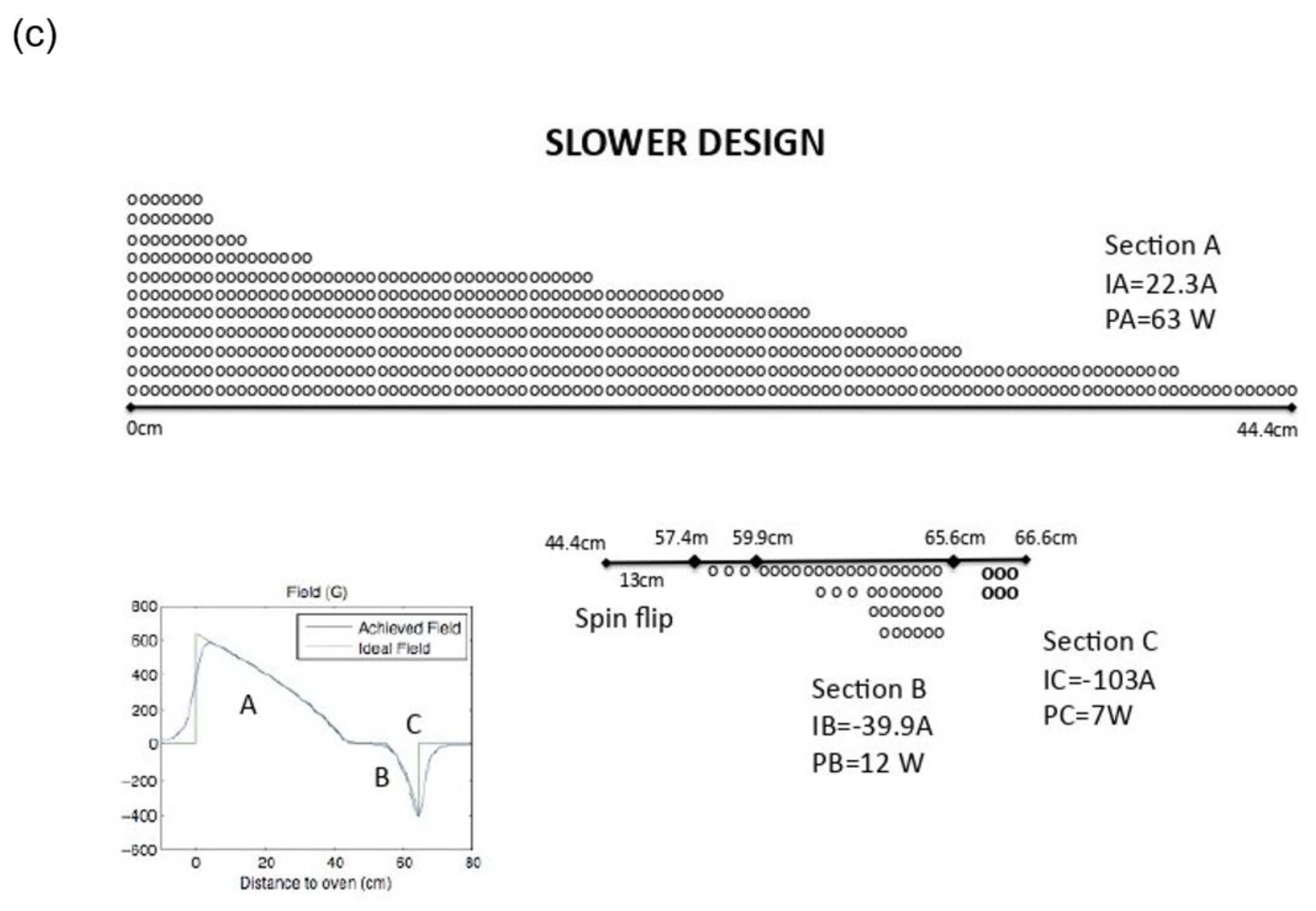
2.2. Spin-Flip Zeeman Slower

In order to have a large flux atom to trap, we need to slow a significant fraction, typically 2/3 (or more) of the Boltzmann distribution of velocities characterizing the atoms leaving the oven. In the case of a field increasing slower for Li-7, this would require large magnetic fields (i.e., 1000 G or more), which can introduce magnetic fringing at the trap position, located close to the end of the slower. A spin-flip slower can be designed in order to reduce the magnitude of the field close to the trap. The main idea is to design a field decreasing (B_ini = 600 G) first section, a zero field (or spin-flip) middle section and a field increasing final section (B_final = −400 G). By adjusting the laser detuning (600 MHz for our species) and the initial and final fields, it is possible to achieve a field profile with a final B-field of only a few hundred G near the vacuum chamber.

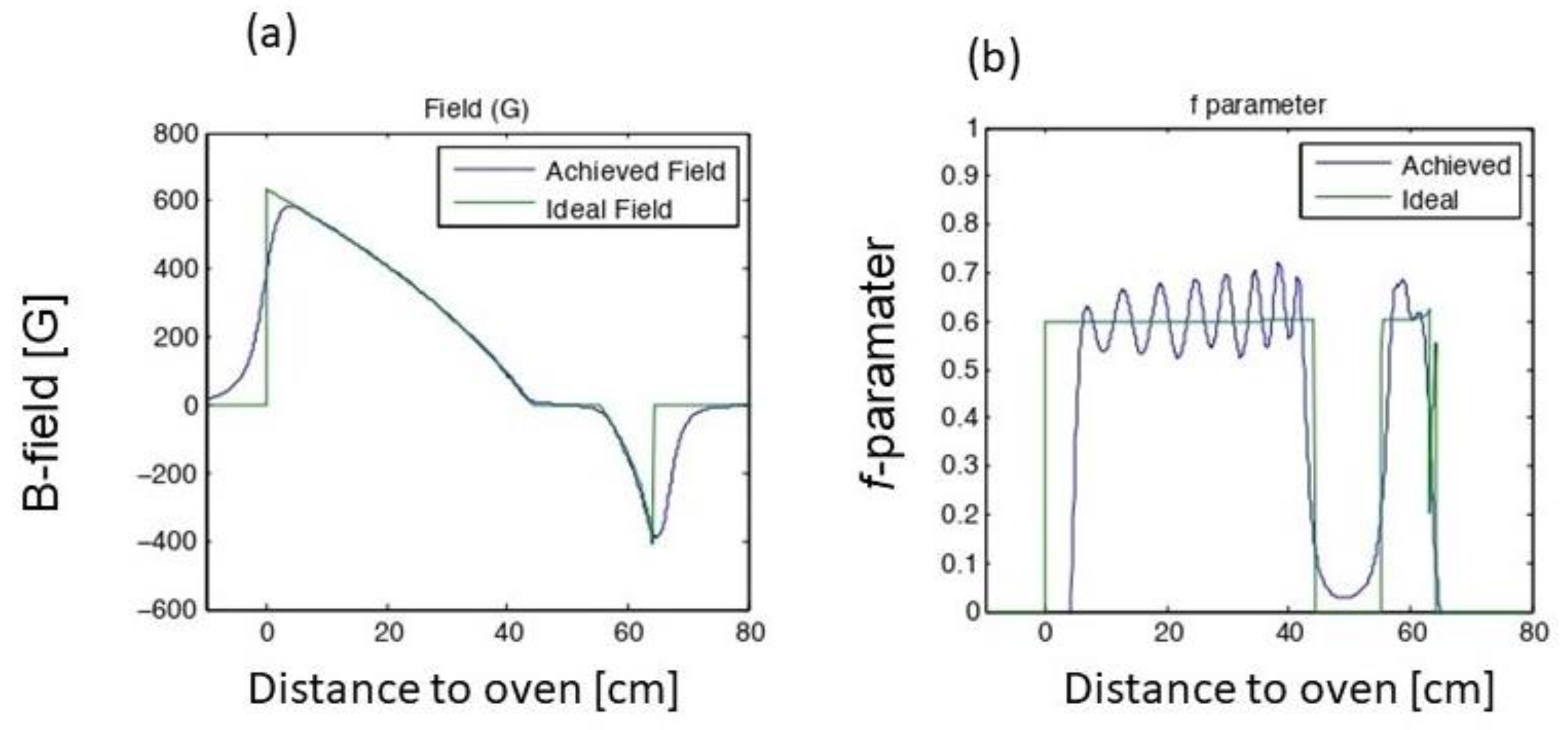
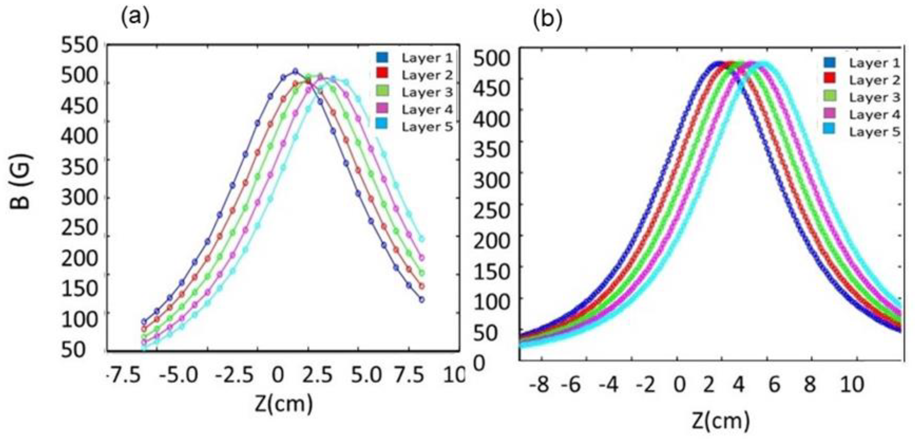
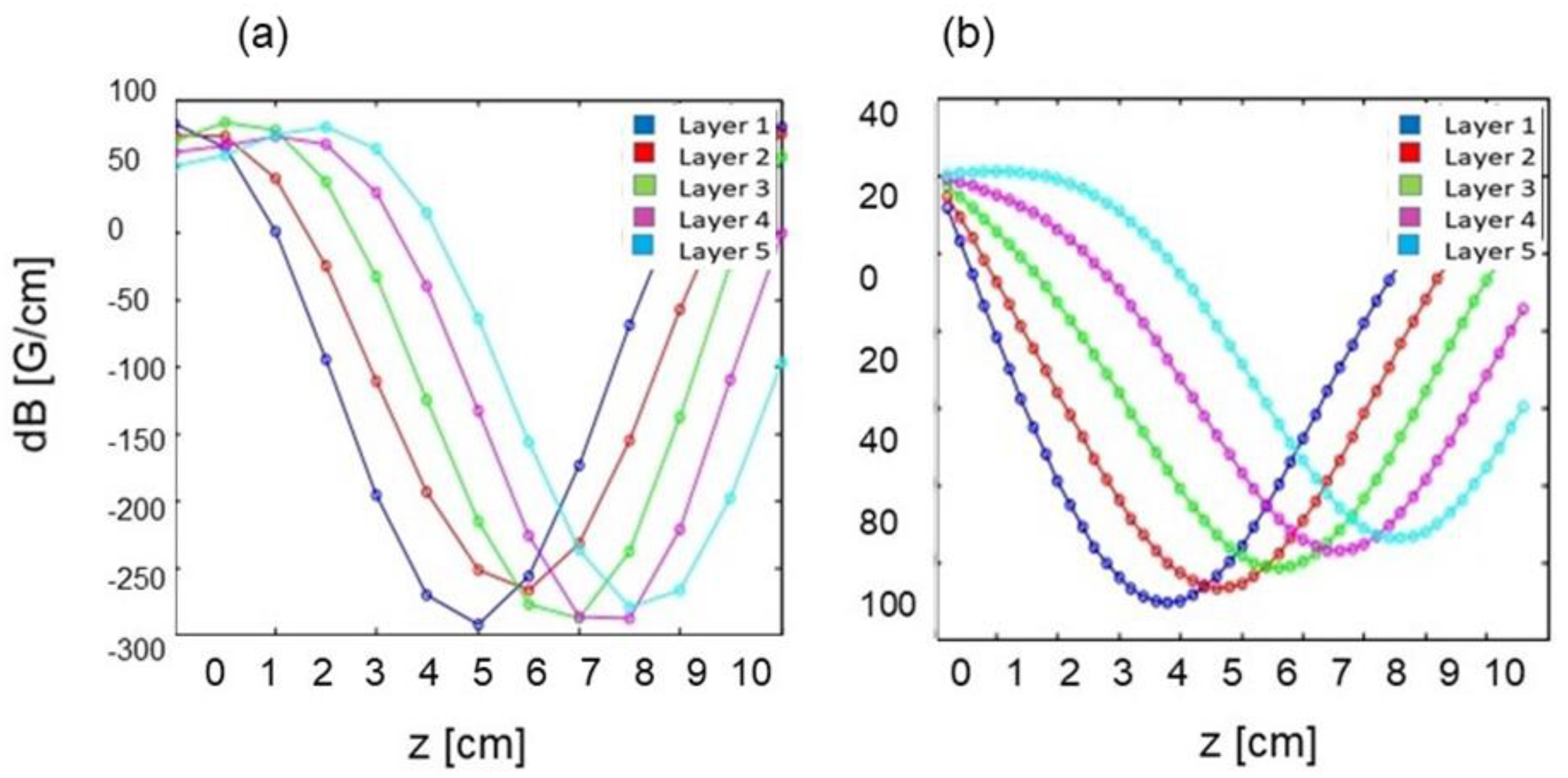
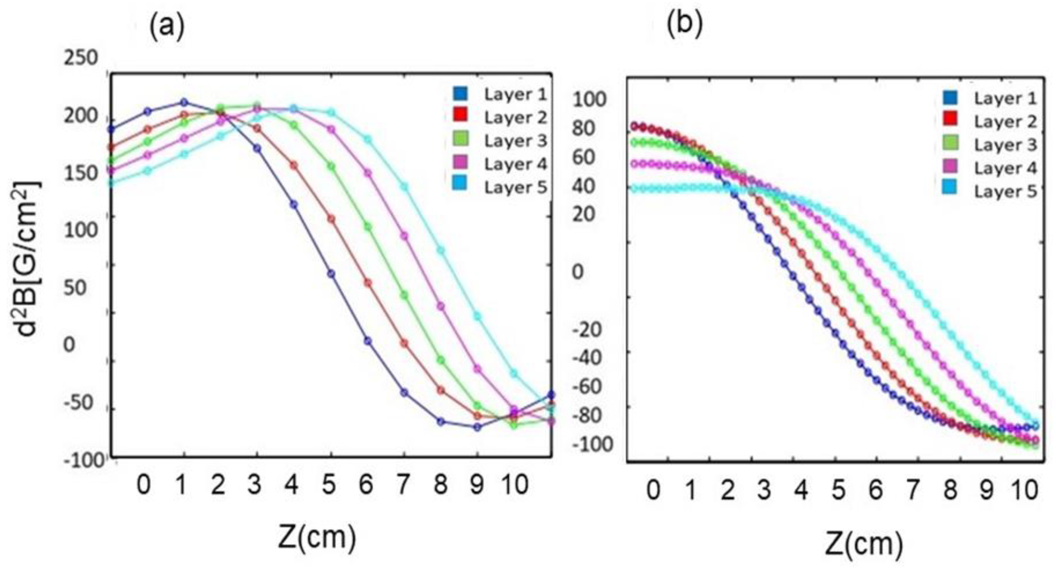
2.3. Simulations

The main criteria to decide if a Zeeman slower design is good enough is that the difference between the ideal field and the field achieved by a winding a set of coils of different radii should be less than the atomic line-width (i.e., 5.9 MHz in the case of Li-7 D2 line, which, in terms of B-field, corresponds to approximately 5 G). Next, the acceleration along the slower should remain lower than the maximum Doppler acceleration (a_max) [12,13], or, in other words, the parameter f = a/a_max should remain smaller than 1 and fluctuate by less than 20% around the chosen target design parameter (f = 0.6 in our case) since large fluctuations in f could produce atom losses.

The results for our numerical simulation of the B-field profile and f-parameter are shown in Figure 1a,b, respectively. As shown in Figure 1c, the design consists of three sections (A, B, C). The first section (A) is the field decreasing part and requires 11 layers with a number of turns ranging from 116 to 7. The current used for this first section in the simulations was I = 23 A. Next, there is the B = 0 or spin-flip segment (B). The length of this segment is eventually determined by the length of the mechanical bellows. The last section (C) corresponds to the decreasing part of the slower. The first part of this last section consists of a few turns with double spacing (weak turns) followed by four layers with and increasing number of turns from 7 to 18. The current used for this second section was I = 40 A.

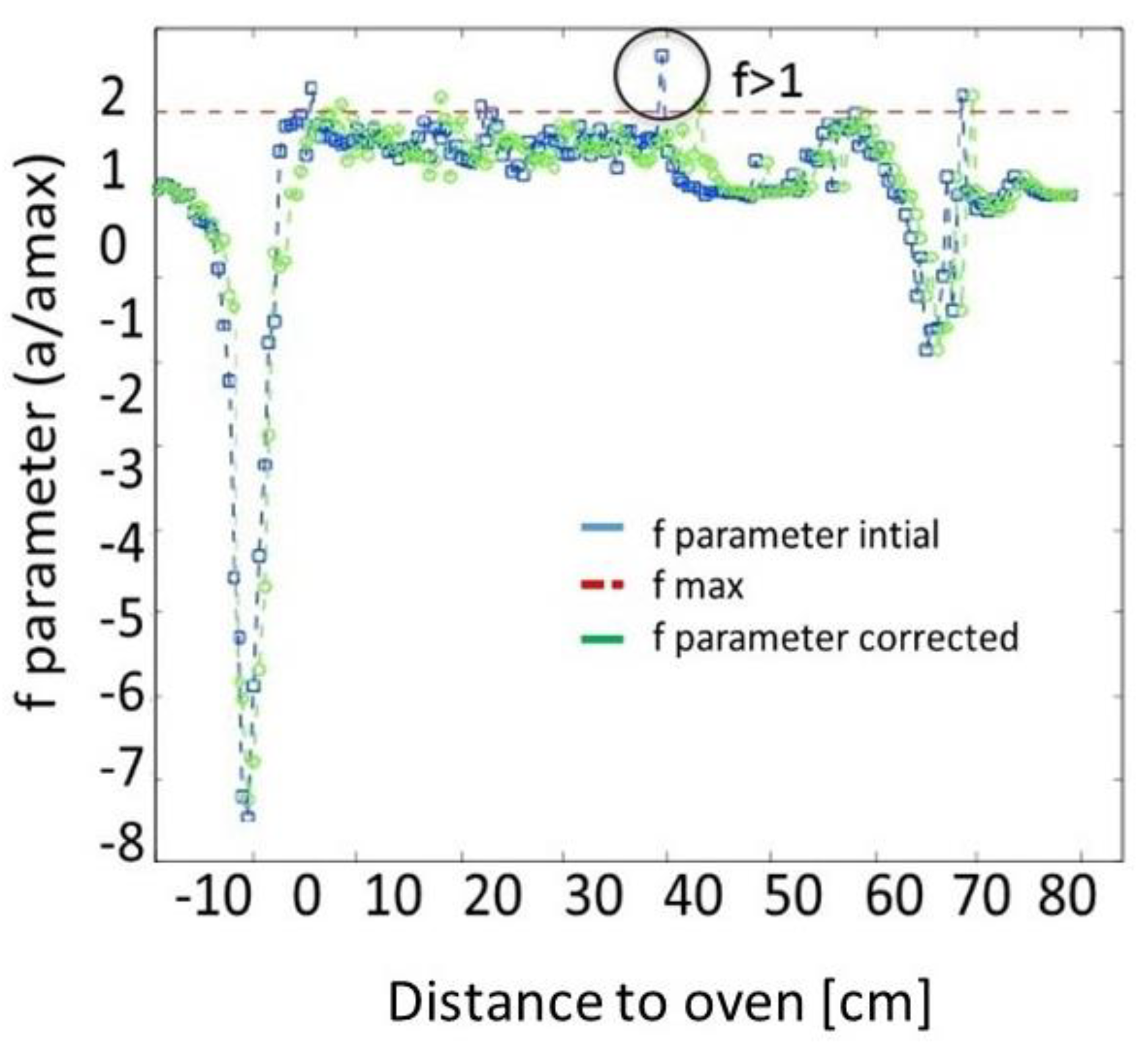
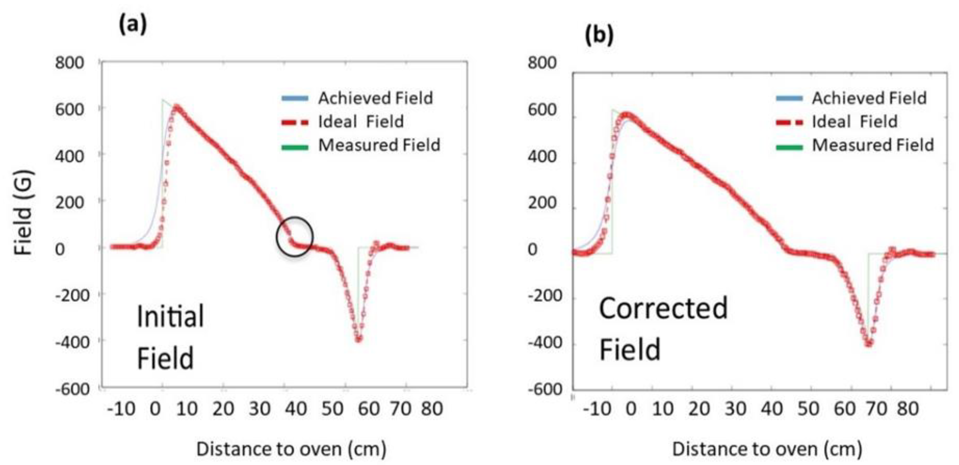
2.4. Slower Measurements

We measured the field by probing the slower with a small current (3 A) for each section in series. In order to prevent regions along the slower with this acceleration, a > a_max, we measured the f parameter (Figure 2) and found that at a specific position (z = 40 cm) f had an “unphysical” peak (f > 1). This peak coincided with the ending of the decreasing section of the slower. We corrected for this by adding one additional turn. Figure 3 shows a comparison between the initially measured field (a) and the corrected field (b).

3. Quadrupole Magnetic Trap

The quadrupole magnetic trap consists of two coils of opposite currents, which produce a magnetic field whose magnitude |B| increases (from zero) with the distance from the center of the trap. The main considerations in designing a quadrupole trap are the separation between coils (∆z), the inner radius of the coils (R), and the number of turns N. In order to fit the coils in our existing bucket windows, the separation should be ∆z = 3.81 cm, and the maximum outer radius should be 16.51 cm. For thick copper wire (0.47625 cm), this corresponds to N = 8 or 9. Additionally, there is a limitation in the number of layers that can be added due to water cooling considerations. Our aim is to cool each layer separately so that each layer can have its own independent current. Taking this into account, 5 layers is approximately the maximum number that we can consider.

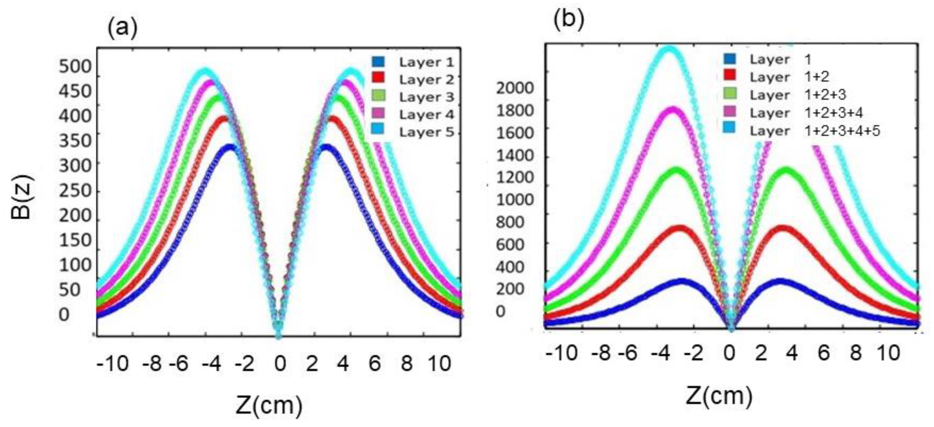
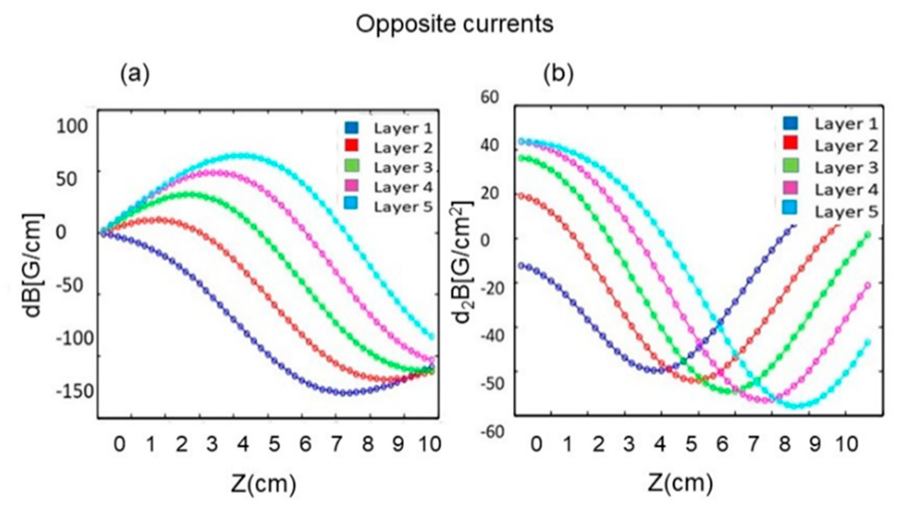
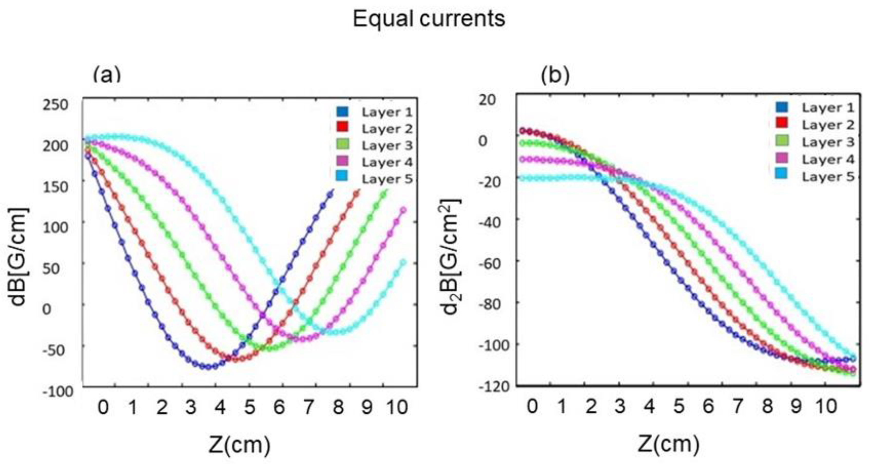
3.1. Field Simulations

The axial magnetic field from a single coil of radius R perpendicular to the z axis, centered at z = A, can be written as [14]:

$$B_Z\left(r,z\right)=\frac{{\mu }_{0}I}{2\pi }\frac{1}{{[{\left(R+Z\right)}^2+{\left(Z-A\right)}^2]}^{1/2}}\times E\left(k^2\right)$$

(4)

where E(k²) is an elliptical integral [1], with μ₀ = 4π × 10⁻⁷, for vacuum and SI units and k² = [4Rr/(R + r)² + (R − A)²]. In order to ease the notation, we shall call B the z-component of the magnetic field in the rest of the manuscript.

3.2. Trap Fields

Consider a design consisting of 5 layers, with 9 turns each, and a current of I = 400 A in each layer. The axial fields due to each layer (B), first derivative ($\frac{dB}{dz}$) and second derivatives ($\frac{d{B}^2}{d{z}^2}$) are shown in Figure 4, Figure 5 and Figure 6, respectively.

The field gradient due to each coil individually is around 150 G/cm and can be used independently. Moreover, these graphs suggest that the total field gradient (i.e., the slope of sum |B|) due to the 5 coils is around 750 G/cm at 400 A (i.e., 1.875 G/cmA), while a field gradient of approx. 0.55 G/cmA is required for trapping Li-7, suggesting that our coils should be appropriate for our application.

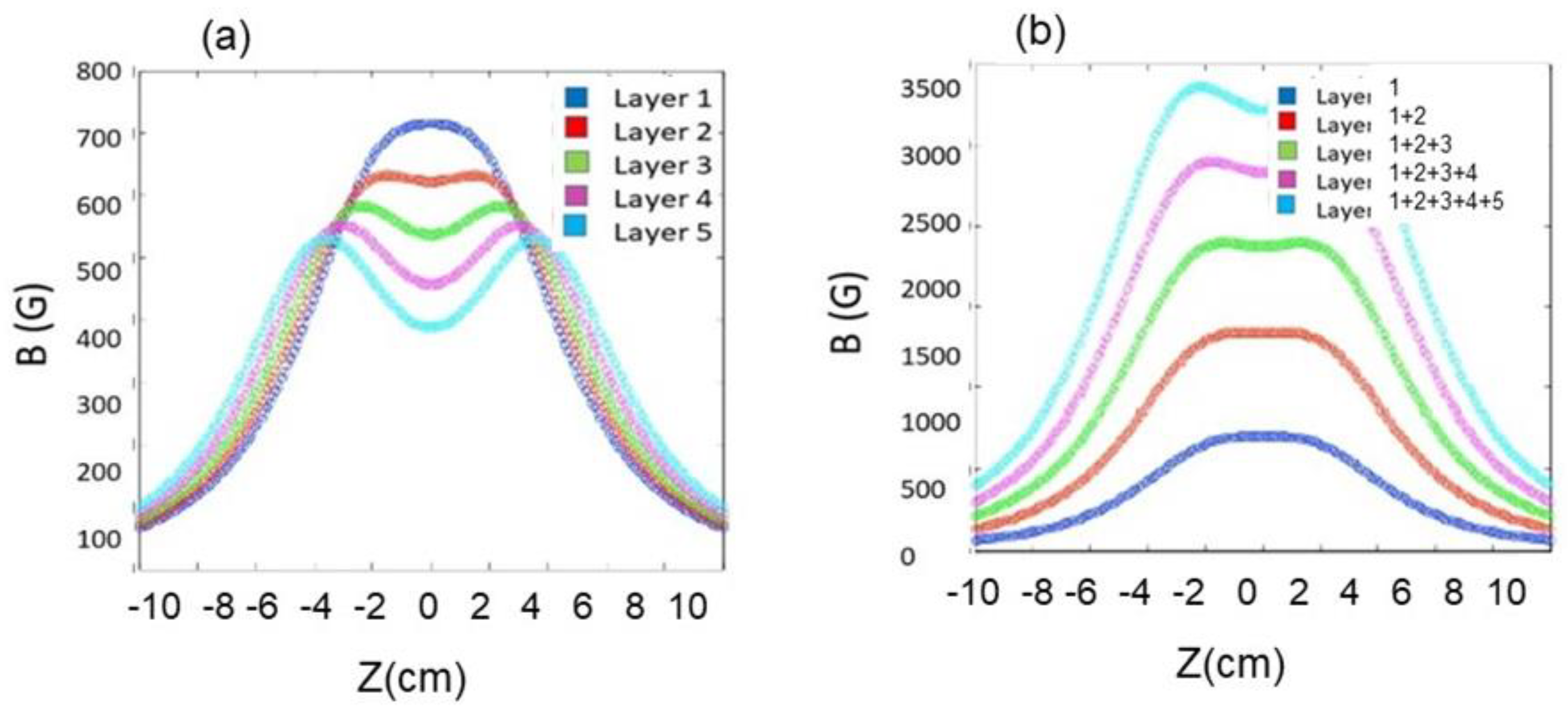
4. Feshbach Fields

The Feshbach fields are obtained using the same coils but sending both currents in the same direction so that |B| is maximum at the center of the trap. It is also important to have zero curvature ($\frac{d{B}^2}{d{z}^2}$ = 0) in the Feshbach field at the trap location, for which the layers in the Helmholtz configuration (R = ∆z) will be used. Note that by adding layers 1 and 2 it is possible to achieve fields of up to 900 G, which seems within the range required for tuning the Li-7 resonances. Simulated Feshbach fields are shown in Figure 7.

Figure 7 shows a simulation of the field that will be used to tune the Feshbach resonances. For this application, it is important that the curvature of the field is as small as possible at the position of the trap z = 0. For this purpose, layers 1 and 2 should be used, since those are the closest to the Helmholtz configuration.

Windings and Measurements

Coil winding can be a very challenging task. One of the main aspects to take into account is that the spacing between coils should be as small as possible and the layers should be as 2D as possible. This means that it is necessary to introduce a lot of pressure and tension in the system, especially during the large amount of time it takes for the Epoxi glue to cure (6 h approximately).

We measured the fields, on each layer in each coil, by sending a small current (5 A) and then rescaling it. This is presented in Figure 8a,b and shows the corresponding numerical simulation. The error in the field is within 10%, as expected due to small deviations in the shape of coils by bending and additional Epoxi. In order to find the first and second derivatives of the measured field at the trap position and then obtain the values for the gradient field and curvature, we fitted the fields with a polynomial expansion [14,15,16,17,18]:

$$y={\displaystyle \sum }_{n=0}{b}_n{x}^n$$

(5)

Once we obtained the fitting coefficients b_n, we calculated the first and second derivatives. Figure 9 shows the measured (a) and simulated (b) first derivative of the field $\frac{dB}{dz}$ (G/cm). The actual position of the trap in (a) is 1.905 cm from z = 0. Agreement between numerical simulations and experimental results is apparent.

Figure 10a Shows the second derivative of the polynomial fit to measured fields $\frac{d{B}^2}{d{z}^2}$ (G/cm²), and Figure 10b shows the corresponding numerical simulations. The qualitative agreement between numerical simulations and experimental results is revealed. The measured curvatures appear to range between 25 and 75 G/cm². The curvature of the field can eventually be corrected by running a small negative current in the outermost layer.

5. Discussion

The comparison between the experimental results and numerical simulations presented in Figure 8, Figure 9 and Figure 10 reveal the qualitative agreement between experiment and theory. From Figure 8, we note that there is roughly a 10% difference in the magnitude of the measured field (Figure 8a, B_max = 500 G) and simulated fields (Figure 8b, B_max = 450 G), this error can be ascribed to bias noise, limited precision, Gaussmeter calibration errors, in addition to probe alignment errors. We attribute the difference in the scales presented in the theoretical and numerical plots to such probe alignment errors. Experimental errors within 10% in the measured B-field are later propagated in the first and second derivatives of the field for each layer, resulting in roughly 20% and 30% divergence between measured and simulated derivatives of the B-field.

6. Conclusions

We presented the design and construction of the magnetic coils for a new machine for ultra-cold Li-7. In particular, we reported numerical simulations and experimental results for the spin-flip Zeeman slower, quadrupole magnetic trap, and Feshbach fields. This machine will be employed to emulate novel quantum phases of matter and quantum magnetism with ultra-cold Li-7 [19,20,21].

References

- Orzel, C. Quantum Simulation; IOP Publishing Ltd.: Bristol, UK, 2017. [Google Scholar]
- Misguish, G.; Lhuillier, C. Frustrated Spin Systems; World Scientific: Singapore, 2005. [Google Scholar]
- Jacksch, D.; Bruder, C.; Cirac, J.I.; Gardiner, C.W.; Zoller, P. Cold Bosonic Atoms in Optical Lattices. Phys. Rev. Lett. 1998, 81, 3108. [Google Scholar] [CrossRef]
- Duan, L.-M.; Demler, E.; Lukin, M.D. Controlling Spin Exchange Interactions of Ultracold Atoms in Optical Lattices. Phys. Rev. Lett. 2003, 91, 090402. [Google Scholar] [CrossRef] [PubMed]
- Mandel, O.; Greiner, M.; Widera, A.; Rom, T.; Hänsch, T.W.; Bloch, I. Controlled collisions for multi-particle entanglement of optically trapped atoms. Nature 1999, 425, 937. [Google Scholar] [CrossRef]
- Anderlini, M.; Lee, P.J.; Brown, B.L.; Sebby-Strabley, J.; Phillips, W.D.; Porto, J.V. Controlled exchange interaction between pairs of neutral atoms in an optical lattice. Nature 2007, 448, 452. [Google Scholar] [CrossRef] [PubMed]
- Trotzky, S.; Cheinet, P.; Fölling, S.; Feld, M.; Schnorrberger, U.; Rey, A.M.; Polkovnikov, A.; Demler, E.A.; Lukin, M.D.; Bloch, I. Time-Resolved Observation and Control of Superexchange Interactions with Ultracold Atoms in Optical Lattices. Science 2008, 319, 295. [Google Scholar] [CrossRef] [PubMed]
- Jaksch, D.; Briegel, H.-J.; Cirac, J.I.; Gardiner, C.W.; Zoller, P. Entanglement of Atoms via Cold Controlled Collisions. Phys. Rev. Lett. 1999, 82, 1975. [Google Scholar] [CrossRef]
- Streed, E.W.; Chikkatur, A.P.; Gustavson, T.L.; Boyd, M.; Torii, Y.; Schneble, D.; Campbell, G.K.; Pritchard, D.E.; Ketterle, W. Large atom number Bose-Einstein condensate machines. Rev. Sci. Instrum. 2006, 7, 023106. [Google Scholar] [CrossRef]
- Stan, C.A. Experiments with Interacting Bose and Fermi Gases. Ph.D. Thesis, Massachusetts Institute of Technology, Cambridge, MA, USA, 2005. [Google Scholar]
- Stan, C.A.; Ketterle, W. Multiple species atom source for laser-cooling experiments. Rev. Sci. Instrum. 2005, 76, 063113. [Google Scholar] [CrossRef]
- Foot, C. Atomic Physics; Oxford Univ. Press: Oxford, UK, 2005. [Google Scholar]
- Metcalf, J. Laser Cooling and Trapping; Springer: Cham, Switzerland, 1999. [Google Scholar]
- Bergeman, T.; Erez, G.; Metcalf, H. Magnetostatic trapping fields for neutral atoms. Phys. Rev. A 1987, 35, 1535. [Google Scholar] [CrossRef] [PubMed]
- Montgomery, D. Solenoid Magnet Design; Wiley-Interscience: New York, NY, USA, 1969. [Google Scholar]
- Streed, E.W. 87-Rb Bose-Einstein Condensates: Machine Construction and Quantum Zeno Experiments. Ph.D. Thesis, Massachusetts Institute of Technology, Cambridge, MA, USA, 2006. [Google Scholar]
- Davis, K.B.; Mewes, M.O.; Andrews, M.R.; van Druten, N.J.; Durfee, D.S.; Kurn, D.M.; Ketterle, W. Bose-Einstein condensation in a gas of sodium atoms. Phys. Rev. Lett. 1995, 75, 3969. [Google Scholar] [CrossRef] [PubMed]
- Petrich, W.; Anderson, M.H.; Ensher, J.R.; Corne, E.A. Stable, tightly confining magnetic trap for evaporative cooling of neutral atoms. Phys. Rev. Lett. 1995, 74, 3352. [Google Scholar] [CrossRef] [PubMed]
- Moulieras, S.; Lewenstein, M.; Puentes, G. Entanglement engineering and topological protection by discrete-time quantum walks. J. Phys. B At. Mol. Opt. Phys. 2013, 46, 104005. [Google Scholar] [CrossRef]
- Huh, S.; Kim, K.; Kwon, K.; Choi, J. Observation of a strongly ferromagnetic spinor Bose-Einstein condensate. arXiv 2020, arXiv:2006.06228. [Google Scholar]
- Dimitrova, I.; Lunden, W.; Amato-Grill, J.; Jepsen, N.; Yu, Y.; Messer, M.; Rigaldo, T.; Puentes, G.; Weld, D.; Ketterle, W. Observation of two-beam collective scattering phenomena in a Bose-Einstein condensate. Phys. Rev. A 2017, 96, 051603. [Google Scholar] [CrossRef]
© 2020 by the author. Licensee MDPI, Basel, Switzerland. This article is an open access article distributed under the terms and conditions of the Creative Commons Attribution (CC BY) license (http://creativecommons.org/licenses/by/4.0/).
Share and Cite
Puentes, G. Design and Construction of Magnetic Coils for Quantum Magnetism Experiments. Quantum Rep. 2020, 2, 378-387. https://doi.org/10.3390/quantum2030026
Puentes G. Design and Construction of Magnetic Coils for Quantum Magnetism Experiments. Quantum Reports. 2020; 2(3):378-387. https://doi.org/10.3390/quantum2030026
Chicago/Turabian StylePuentes, Graciana. 2020. "Design and Construction of Magnetic Coils for Quantum Magnetism Experiments" Quantum Reports 2, no. 3: 378-387. https://doi.org/10.3390/quantum2030026
APA StylePuentes, G. (2020). Design and Construction of Magnetic Coils for Quantum Magnetism Experiments. Quantum Reports, 2(3), 378-387. https://doi.org/10.3390/quantum2030026