Article

Correlations between Complexity and Entanglement in a One-Dimensional XY Model

1
Departamento de Física, Facultad de Ciencias, Universidad Católica del Norte, Angamos 0610, Antofagasta 1270709, Chile
2
Departamento de Física, Facultad de Ciencias Exactas y Naturales, Universidad Nacional de La Pampa, CONICET, Av. Peru 151, Santa Rosa 6300, Argentina
3
Department of physics, National University La Plata-CONICET-IFLP, CC 727, La Plata 1900, Argentina
*
Author to whom correspondence should be addressed.
Quantum Rep. 2020, 2(2), 305-313; https://doi.org/10.3390/quantum2020020
Submission received: 28 April 2020 / Revised: 13 May 2020 / Accepted: 18 May 2020 / Published: 24 May 2020

Abstract

:
Many people believe that the study of complex quantum systems may be simplified by first analyzing the static and dynamic entanglement present in those systems [Phys. Rev. A 66 (2002) 032110]. In this paper, we attempt to complement such notion by adding an order–disorder quantifier called statistical complexity and studying how it is correlated with the degree of entanglement as measured by the concurrence quantifier. We perform such an analysis with reference to a representative system chosen from condensed matter theory, the so-called X Y model. Some interesting insight is obtained as the concurrence and the complexity become correlated in an unexpected fashion.

1. Introduction

Many people believe that the study of complex quantum systems may be simplified by first analyzing the static and dynamic entanglement present in those systems [1,2,3]. We wish here to conjoin such sensible notion with the ideas underlying the concept of statistical complexity (SC) advanced in Ref. [4] (see also, for instance, Refs. [5,6,7,8,9,10,11,12,13,14,15,16,17,18,19,20,21], as a small sample). The SC notion is widely employed today, mostly in connection with systems for which statistical mechanics and thermodynamics happen to provide adequate theoretical study-tools. To conjoin SC with entanglement is expected by us to make sense because of the development in the last 20 years of quantitative high-level principles governing the behavior of entangled states, independent of their particular physical representation. The pertinent principles are said to be analogous to the laws of thermodynamics [1]. Thus, the correlation that we seek should plausibly exist.
It was suggested in Ref. [1] that the complexity in quantum systems is closely bound up to the entanglement between its constituent parts. This paper laddresses this very issue by means of an important tool known as the statistical complexity measure, which will be used here to study what its connection is with the degree of entanglement associated between spins of an 1D X Y chain. Note that the entanglement notion is useful within the quantum mechanics’ domain. On the other hand, the application domain of the statistical complexity formalism transcends the quantum theory limits, since it can be used in a classical system as well. The statistical complexity measure has been successfully tested in different systems [10,11,13,14,15,16,17,18,19,20,22]. Here, we study the complexity in a quantum 1D transverse X Y model, which is interesting for several reasons. Firstly, the X Y chain possesses an exact solution. Second, being a low dimensional system, the quantum fluctuations play a prominent role in its properties. Third, these fluctuations compete with the order tendency, and, in many cases, lead to a behavior quite different from that observed for systems with higher dimensionality. It is this last feature that makes a 1D X Y model an interesting subject to study from the SC-point of view, since this formalism is able to capture the order–disorder balance of a given system [5,6,7,8,9,10,11,12,13,14,15,16,17,18,19,20,21].

1.1. Motivation

The authors of Ref. [1] hoped that the quantitative theory of entanglement could provide a powerful unifying framework for the understanding of complex quantum systems. This is so because, when viewed in terms of their entanglement content, a large number of apparently different states turn out to be equivalent.
This present paper is one step for testing such hypothesis. Consequently, we ask ourselves here whether concurrence (an entanglement monotone) and SC are indeed correlated, and, if so, how.

1.2. Our Goal

We will show that the answer we seek is in the positive and will provide interesting insight. We will work with reference to the celebrated X Y model (see Ref. [1] and references therein). The signature of complexity in this system is the occurrence of a quantum phase transition [1]. We will quantify the entanglement of formation [23,24,25,26] in terms of another entanglement measure, the concurrence C (as stated above, the entanglement of formation varies monotonically with the concurrence) [23,24,25,26].
The work is organized as follows: Section 2 introduces some necessary preliminary materials. Section 3 describes the X Y -model. Our results are presented in Section 4 and some conclusions are drawn in Section 5.

2. Meaning of the Statistical Complexity Measure

One would like, in many instances, to adequately grab hold of a system’s correlation-structures in the same manner in which the entropy-notion grasps disorder. In other words, to be in a position to capture the precise relationship amongst the variegated components of a given system. Why? Mainly because such correlations greatly influence the principal features of the particular probability distribution (PD) describing some physical process one is interested in. Now, the pair randomness structural correlations do not exhibit totally independent ingredients.
We are confident that the contrasting extremes of (i) perfect order and (ii) maximal randomness should not manifest important structural correlations [4]. In between these two opposite instances, a considerable range of structural degrees (SD) should exist. These SD ought to be manifested by the traits of the PD of the preceding paragraph. Exactly how would be the question at this point. As Crutchfield stated in 1994, “Physics does have the tools for detecting and measuring complete order equilibria and fixed point or periodic behavior and ideal randomness via temperature and thermodynamic entropy or, in dynamical contexts, via the Shannon entropy rate and Kolmogorov complexity. What is still needed, though, is a definition of structure and a way to detect and to measure it” [5,6]. Seth Lloyd counted as many as 40 manners of defining complexity, none of them quite satisfactory [27].
In Ref. [4], its authors concocted a quite appropriate functional F [ P ] that can capture correlations in a fashion similar to that of how Shannon’s entropy captures randomness. This constituted a major breakthrough and was mathematically conceptualized via the definition advanced by López-Ruiz, Mancini, and Calbet (LMC) [4], which they called the statistical complexity C. LMC C clearly separated and quantified the contributions of entropy and structure, the latter being described by a notion called disequilibrium D. Their statistical complexity was widely acclaimed (see, for a small sample, Refs. [7,8,9,10,11,12,13,14]). C vanishes in the two special extreme instances of perfect order and maximum disorder mentioned above. C is defined as the product of the entropy S and the disequilibrium D where the latter is a distance measure in probability space, between the actual PD and the unform distribution. Therefore, C is of the form
C = S D ,
where the well-known Shannon entropy is
S = i p i ln p i ,
and the disequilibrium is defined as [4]
D = i ( p i 1 / N ) 2 ,
where p 1 , p 2 , , p N are the corresponding probabilities.
To picture a typical form of certain C -graphs, suppose that x is the “ordering parameter” of a system, such that, at x = 0 , the system displays perfect order, and, at x = b , total randomness prevails. In a naive model, if C = x 2 b x , one attains a maximum for C at x = b / 2 . This situation is typical of what happens in variegated systems, where C is of course a functional of the probability distribution and x some parameter like the temperature [7,13]. In a more realistic vein, the statistical complexity and the disequilibrium have recently been shown to be telltale of superconductivity [15] or to give indications regarding the Schottky effect [16], the coriolis-antipairing effect [17], or the classical-quantum frontier [18]. One of the simplest types of quantum correlations, those present in gaseous systems due to symmetry considerations, were fruitfully analyzed using D in Ref. [20]. In addition, the statistical complexity and the disequilibrium turn out rather surprisingly apt at providing significant insights into few fermion-model characteristics [19]. Even more, in a classical, canonical-ensemble environment, D is able to replace the partition function [14].

3. The XY Model

We consider an isotropic X Y model in a one-dimensional, lattice [1,28]. It has N sites, with periodic boundary conditions, in a transverse magnetic field h. The pertinent Hamiltonian is [1]
H = j = 1 N λ 2 ( σ j x σ j + 1 x + σ j y σ j + 1 y ) + h σ j z λ 2 σ N x σ 1 x + σ N y σ 1 y ,
where σ j α ( α = x , y , z ), is the Pauli matrix at site j. The parameter λ controls the strength of the coupling between first neighboring spins. In addition, λ > 0 ( λ < 0 ) corresponds to ferromagnetic (anti-ferromagnetic) coupling [1]. We set the value of Planck’s constant at = 1 and the Boltzmann constant k B = 1 (in energy units). The magnetic field is denoted by h. The parameter λ and the temperature T have dimensions of energy and are measured in h units.
The exact solution of the N sites- X Y model was derived through the Jordan–Wigner transform, which can be consulted in Ref. [29]. Following the process described there, one finds a diagonalized Hamiltonian, expressed in terms of the Jordan–Wigner fermionic operators η q and whose appearance is [1]
H = 2 q ω q η q η q q ω q ,
where ω q = | 1 + λ cos ϕ q | is the energy per site, with ϕ q = 2 π q / N [1]. Note that we have adopted a notation slightly different from that of the reference mentioned above.

3.1. The Statistical Complexity Applied to the X Y Model

If our system is in thermal equilibrium at temperature T, the pertinent diagonal density matrix in the canonical ensemble is given by [1]
ρ = e β H / Z ,
with Z = Tr exp ( β H ) the partition function. For our purpose, we need an important quantity, that is, the Helmholtz free energy which is defined as
F = T N ln Z .
In the thermodynamic limit, N , sums that appear in the expectation values are replaced by integrals. Thereby, it is convenient to change the discrete variable q by the continuous variable ϕ . In this way, the corresponding Helmholtz free energy for the X Y model in this limit, given in Refs. [28,30], reads
F = ε 0 T 2 π π π d ϕ ln ( 1 + exp ( 2 | λ cos ϕ + 1 | / T ) ) ,
where ε 0 is given by
ε 0 = 1 2 π π π d ϕ | λ cos ϕ + 1 | .
Remember that we have taken h = 1 in all expressions above.
Once we have F (explicitated in Equation (8)), we calculate C following the route traced in Refs. [14,31], where the Helmholtz free energy F was considered. Then, from F, one obtains the disequilibrium D as follows [14,31]:
D = exp [ 2 β ( F ( T ) F ( T / 2 ) ) ] .
Using ln Z , one also finds the entropy S, as prescribed by any textbook, so that we have a statistical complexity C x
C x = S D .
This last expression, together with Equation (10), will be computed below.

3.2. Site-Concurrence in the X Y Model

The density matrix ρ stores all the needed information about the correlations between any bi-partition of a given system appropriate for entanglement discussions. In the case of a system in thermal equilibrium at temperature T, the density matrix is given by Equation (6) [1].
In a quantum system, much stronger correlations between observables exist than those allowed in classical physics. This kind of quantum correlation, which does not have a classical analog, is usually called entanglement (see Ref. [1] and references therein). There are many entanglement measures [1]. Some of them involve the evaluation of a reduced density matrix ρ of the bipartite system S = A B [1]. The reduced density matrix of such a system, corresponding to the sub-part A (B), is defined by ρ A = tr B ( ρ ) ( ρ B = tr A ( ρ ) ), where tr B ( · ) ( ρ B = tr A ( · ) ) means trace over B (A) degrees of freedom [1].
Let us define the partial trace E i , j over all sites of the X Y chain but the ith and jth ones. The two point reduced density matrices are defined by ρ i j = tr E i , j ( ρ ) . As pointed out in Ref. [1], appeal to the calculation of the two point reduced density ρ i , j from ρ in their diagonal representation, like the one in Equation (6), is not the best starting point because it involves quite complicated non-local functions of the original spin operators. Fortunately, there is an alternative approach, based on the one-to-one correspondence between ρ i , j and two-spin correlations at the corresponding sites [1]. The two point density operator ρ i j is represented by a four by four Hermitian matrix, and the number of real parameters needed to specify it are fifteen. Specifically, any four by four density matrix can be written as a linear combination of tensor products σ i α σ j β [1],
ρ i j = α , β = 0 3 w α β σ i α σ j β 4 ,
where σ i 0 denotes the 2 × 2 identity matrix and the three σ i 1 σ i x , σ i 2 σ i y , σ i 3 σ i z are the Pauli matrices associated with the ith site.
From the orthonormal relation tr ( σ i α σ j β · σ i ν σ j μ ) = δ α β , ν μ , it follows that the coefficients of the one-point reduced density operators are given by [1],
w α β = tr ( ρ i j σ i α σ j β ) = σ α i σ β j .
Note that the Equations (12) and (13) are nothing but the one-to-one correspondence between the two-point correlations and the two-point reduced density operators. In particular, from the condition tr ( ρ i j ) = 1 , it follows that the coefficient w 00 = 1 . The procedure can be efficiently implemented by considering the symmetries of the X Y Hamiltonian. Specifically, the translation invariance entails that the average values of (1) spin operators and (2) the one spin reduced density matrix do not depend on the sites’ location, i.e, σ i = σ 0 . On the other hand, the translation invariance and reflection symmetry imply that the spin–spin correlations as well as the two spin reduced density matrix depend on the distance between the two spins; that is to say, σ i σ j = σ l σ 0 and ρ i , j = ρ 0 , l ( r = | i j | ). As a consequence of Equation (6), the thermal density operator ρ inherits the Hamiltonian symmetry. Since our Hamiltonian is invariant under the global transformation σ i x σ i x or σ i y σ i y , the same is true for ρ . It follows from this fact that some coefficient of ρ i j should vanish, specifically, the coefficients w 1 = σ i x = 0 , w 2 = σ i y = 0 , and w α β = σ i α σ j β = 0 if α β .
Following Ref. [1], the two point reduced density matrix is
ρ 0 r = I 0 I r + σ z ( σ 0 z I r + I 0 σ r z ) + k = 1 3 σ 0 k σ r k σ 0 k σ r k 2 ,
where the expectation value σ z in thermal equilibrium is given by [1]
σ z = 1 π 0 π d ϕ 1 + λ cos ( ϕ ) ω ϕ tanh 1 2 β ω ϕ ,
and the two spin correlation functions are given by [1],
σ 0 x σ r x = G 1 G 2 G r G 0 G 1 G r + 1 G r 2 G r 3 G 1 ,
σ 0 y σ r y = G 1 G 0 G r + 2 G 2 G 1 G r + 3 G r G r 1 G 1 ,
σ 0 z σ r z = σ z 2 G r G r ,
where
G r = 1 π 0 π d ϕ 1 + λ cos ( ϕ ) ω ϕ cos ( ϕ r ) tanh 1 2 β ω ϕ .
Once obtained, with the reduced matrix ρ 0 r , one can calculate the concurrence between two sites separated by r lattice constants. The concurrence C is a measure of the degree of entanglement between two qubits (here two sites) applicable for both pure and mixed states. The concurrence associated with the state ρ 0 r is given by [1]
C ( ρ 0 r ) = max { 0 , λ 1 λ 2 λ 3 λ 4 } ,
where the λ i ’s are the square root eigenvalues of the operator ρ 0 r ρ ˜ 0 r , arranged in decreasing order. The operator ρ ˜ 0 r results from applying the spin-flip operation to ρ 0 r ,
ρ ˜ 0 r = ( σ y σ y ) ρ 0 r * ( σ y σ y ) ,
where the matrix ρ 0 r * is the complex conjugate of ρ 0 r .
In the present work, we limit ourselves to the first neighbors’ site-entanglement.

4. Present Results

First, remember the crossover notion. We speak of a smooth transition between separate phases of matter that take place whenever some parameter (thermal/non-thermal) varies. Distinctively, this happens in a region of the associated “phase space”, not at a singular point.
We present our main results in this section. Figure 1 displays, for several temperatures, the nearest neighbor concurrence versus λ for a magnetic field h = 1 . At temperature T = 0 , the picture is somewhat reminiscent of that for the occupation number in a Fermi gas, if we plot site-concurrence versus ( 1 / λ ). In a sense, this fact might be associated with the fact that our sites could be linked to free spinless fermions [1,30]. The site-entanglement-phase transition takes place at λ = 1 . Instead, for finite T, we have a crossover at λ 1 .
Here, we wish to highlight the concomitant counter intuitive notion that temperature is clearly seen to “generate” site-entanglement (orange curve: there is site-entanglement for λ < 1 , which is impossible at T = 0 ). In a sense, we see here a phenomenon already encountered in Ref. [17], in a different context. There it was noted how order can arise out of disorder in originating high-temperature superconductivity. More importantly, Arnesen et al. [32] found that the entanglement between two spins in an antiferromagnetic solid can grow by increasing the temperature.
Note that, at λ 2 , the site-concurrence saturates and no longer changes. One should expect the sites’ associated complexity to vanish after that λ -value is reached. This intuition will be confirmed below.
We now study the behavior of the statistical complexity (SC) versus the coupling constant λ in Figure 2. A pleasant observation can be made.
The SC detects the X Y model’s finite T’s site-entanglement-crossover at λ 1 . This is in line with what happens to phase transitions/crossovers (PTCR) in variegated different systems (see, for instances, Refs. [5,6,7,8,9,10,11,13,14,15,16,17,18,19,20,21]). SC seems to always detect PTCR at their proper location. Just emphasize here, for instance, the Coriolis anti-pairing effect [17].
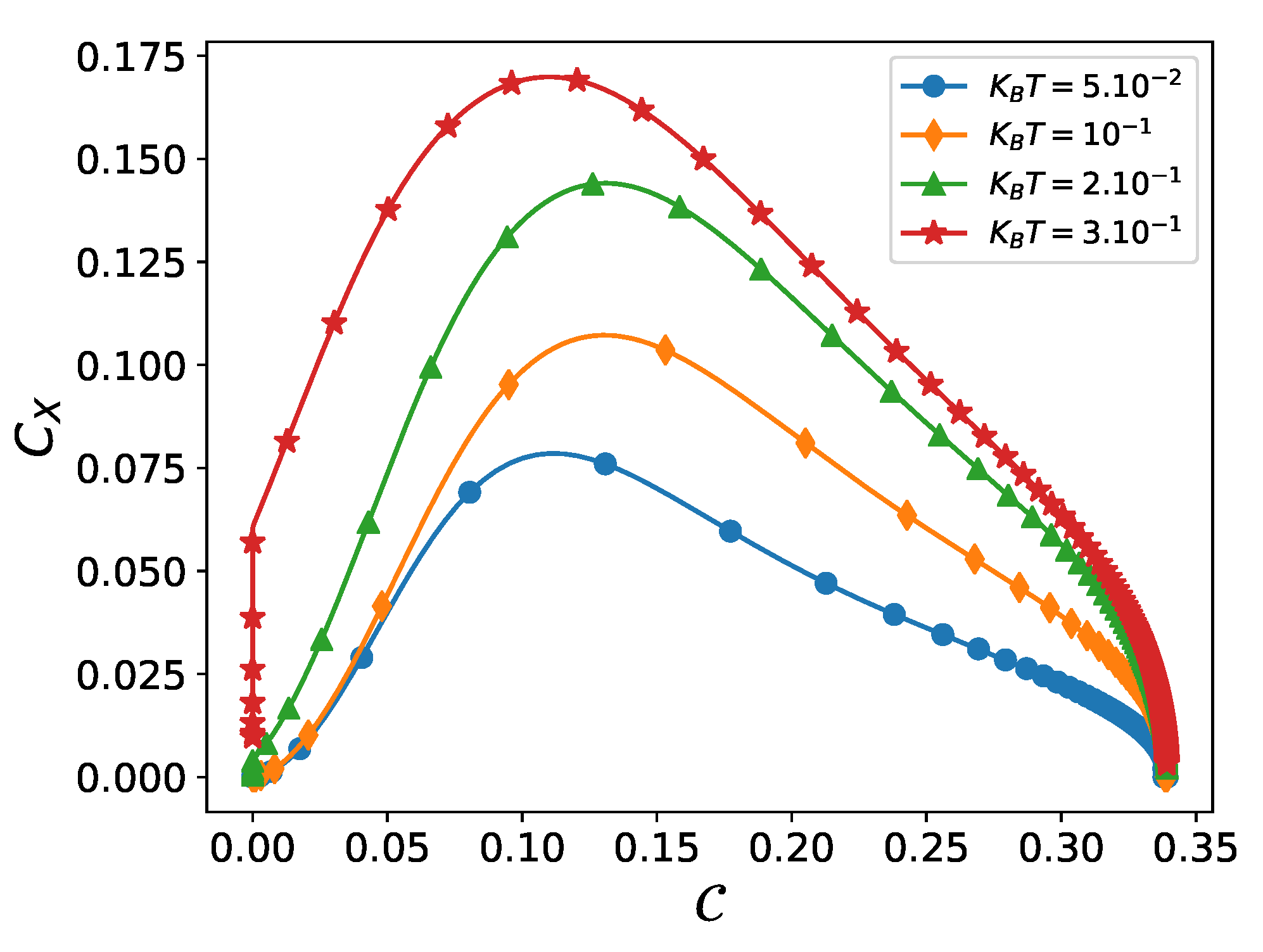
We arrive now to our main present finding. Let z be an order/disorder indicator. One example is the temperature. The intensity of an external magnetic field is other. Then, the plot SC versus z will always have the appearance of Figure 3 [4,5,6,7,8,9,10,11,12,13,14,15,16,17,18,19,20]. Accordingly, it is well known that the SC behaves in this manner:
  • if z is such that the system becomes maximally “ordered”, the SC vanishes.
  • if z is such that the system becomes maximally “disordered”, the SC vanishes.
  • for intermediate z-values, the SC attains a maximum value.
According to Figure 3, the site-concurrence is a z-instance. The graph plots complexity C x ( λ ) versus concurrence C ( λ ) and communicates our main message (it is said that a graph conveys more information than mere words): concurrence is a kind of ordering factor. The complexity vanishes both when C ( λ ) vanishes and when C ( λ ) becomes maximal. This is the typical complexity behavior of [complexity versus an indicator of order/disorder] [4,5,6,7,8,9,10,11,12,13,14,15,16,17,18,19,20]. Figure 3 is indeed a typical graph of C x versus such an order/disorder indicator, as evidenced by perusing the above list of references that encompass variegated physical systems, from the van der Waals gas to superconductivity.
How can we interpret the, at first sight, surprising results of Figure 3? Speaking metaphorically, we could reason as follows:
  • disentangled systems (here sites) A and B are independent ones, like the particles of an ideal gas. The complexity vanishes [4].
  • as two systems (here sites) entangle themselves, they become obviously linked.
  • if the degree of entanglement is high, the separate identities give place to a new entity A + B , with its own features, like a “crystal” with reference to its constituent atoms. The complexity vanishes again [4].
Thus, complexity reflects here on the gradual loss of relative independence of the sites.

5. Conclusions

This effort has shed some new light on the correlation between two physical quantities: (1) site-entanglement (represented by the site-concurrence C ) and (2) statistical complexity by C x .
First, we saw that C x detects, via a nice peak, the site-entanglement crossover at λ 1 .
Generally, C x tends to indicate that something is rapidly varying [4,5,6,7,8,9,10,11,12,13,14,15,16,17,18,19,20]. C x should vanish when change ceases. The novelty here relates to “What is the quantity that changes here?” The answer, surprisingly enough, is entanglement.
More precisely, what gets modified here is C , via the coupling parameter of λ of the X Y model. No coupling entails no site-entanglement and no complexity. Too strong coupling makes C immune to further λ -modification, and the complexity vanishes again. The picture is quite clear to the SC connoisseur. The above-mentioned results entail that site-entanglement can be regarded as a measure of order/disorder, a quite non-trivial conclusion. Large site-entanglement entails a high degree of quantum “order”. Low entanglement would entail, according to this view, quantum “disorder”. Two un-entangled states are separate, unrelated entities. Entanglement makes the two states a single entity with two components that retain a certain degree of “independence”. When entanglement becomes too high, this independence vanishes and complexity as well.

Author Contributions

Conceptualization: A.P. and V.M.A.; Software: D.M.; Investigation: V.M.A., D.M., F.P. and A.P.; formal analysis: V.M.A., D.M., F.P. and A.P.; Validation: F.P. All authors have read and agreed to the published version of the manuscript.

Funding

This research received no external funding.

Acknowledgments

Research was partially supported by FONDECYT, grant 1181558.

Conflicts of Interest

The authors declare no conflict of interest.

References

  1. Osborne, T.J.; Nielsen, M.A. Entanglement in a simple quantum phase transition. Phys. Rev. A 2002, 66, 032110. [Google Scholar] [CrossRef] [Green Version]
  2. Nielsen, M.A. Quantum information theory. arXiv 2000, arXiv:quant-ph/0011036. [Google Scholar]
  3. Preskill, J. Quantum information and physics: Some future directions. J. Mod. Opt. 2000, 47, 127–137. [Google Scholar] [CrossRef]
  4. López-Ruiz, R.; Mancini, H.; Calbet, X. A statistical measure of complexity. Phys. Lett. A 1995, 209, 321–326. [Google Scholar] [CrossRef] [Green Version]
  5. Crutchfield, J.P. The calculi of emergence: Computation, dynamics and induction. Phys. D Nonlinear Phenom. 1994, 75, 11–54. [Google Scholar] [CrossRef]
  6. Feldman, D.P.; Crutchfield, J.P. Measures of statistical complexity: Why? Phys. Lett. Sect. A 1998, 238, 244–252. [Google Scholar] [CrossRef]
  7. Martin, M.; Plastino, A.; Rosso, O. Statistical complexity and disequilibrium. Phys. Lett. A 2003, 311, 126–132. [Google Scholar] [CrossRef]
  8. Kowalski, A.; Martin, M.; Plastino, A.; Proto, A.; Rosso, O. Wavelet statistical complexity analysis of the classical limit. Phys. Lett. A 2003, 311, 180–191. [Google Scholar] [CrossRef]
  9. Rudnicki, Ł.; Toranzo, I.V.; Sánchez-Moreno, P.; Dehesa, J.S. Monotone measures of statistical complexity. Phys. Lett. A 2016, 380, 377–380. [Google Scholar]
  10. López-Ruiz, R. A statistical measure of complexity. In Concepts and Recent Advances in Generalized Information Measures and Statistics; Kowalski, R.A., Rossignoli, E.C., Eds.; Bentham Science Publishers: Sharjah, UAE, 2013; pp. 147–168. [Google Scholar]
  11. Sen, K.D. Statistical Complexity: Applications in Electronic Structure; Springer Science & Business Media: Berlin/Heidelberg, Germany, 2011. [Google Scholar]
  12. Mitchell, M. Complexity: A Guided Tour; Oxford University Press: Oxford, UK, 2009. [Google Scholar]
  13. Martin, M.; Plastino, A.; Rosso, O. Generalized statistical complexity measures: Geometrical and analytical properties. Phys. A Stat. Mech. Its Appl. 2006, 369, 439–462. [Google Scholar] [CrossRef]
  14. Pennini, F.; Plastino, A. Disequilibrium, thermodynamic relations, and Rényi’s entropy. Phys. Lett. A 2017, 381, 212–215. [Google Scholar] [CrossRef]
  15. Pennini, F.; Plastino, A. Complexity and disequilibrium as telltales of superconductivity. Phys. A Stat. Mech. Its Appl. 2018, 506, 828–834. [Google Scholar] [CrossRef]
  16. Pennini, F.; Plastino, A. Disequilibrium, complexity, the Schottky effect, and q-entropies, in paramagnetism. Phys. A Stat. Mech. Its Appl. 2017, 488, 85–95. [Google Scholar] [CrossRef]
  17. Pennini, F.; Plastino, A. Statistical Complexity of the Coriolis Antipairing Effect. Entropy 2019, 21, 558. [Google Scholar] [CrossRef] [Green Version]
  18. Branada, R.; Pennini, F.; Plastino, A. Statistical complexity and classical–quantum frontier. Phys. A Stat. Mech. Its Appl. 2018, 511, 18–26. [Google Scholar] [CrossRef]
  19. Pennini, F.; Plastino, A. Statistical quantifiers for few-fermion’systems. Phys. A Stat. Mech. Its Appl. 2018, 491, 305–312. [Google Scholar] [CrossRef]
  20. Pennini, F.; Plastino, A. Statistical manifestation of quantum correlations via disequilibrium. Phys. Lett. A 2017, 381, 3849–3854. [Google Scholar] [CrossRef] [Green Version]
  21. Anteneodo, C.; Plastino, A.R. Some features of the López-Ruiz-Mancini-Calbet (LMC) statistical measure of complexity. Phys. Lett. A 1996, 223, 348–354. [Google Scholar] [CrossRef]
  22. Ribeiro, H.V.; Zunino, L.; Mendes, R.S.; Lenzi, E.K. Complexity–entropy causality plane: A useful approach for distinguishing songs. Phys. A Stat. Mech. Its Appl. 2012, 391, 2421–2428. [Google Scholar] [CrossRef] [Green Version]
  23. Wootters, W.K. Entanglement of formation and concurrence. Quantum Inf. Comput. 2001, 1, 27–44. [Google Scholar]
  24. Wootters, W.K. Entanglement of formation of an arbitrary state of two qubits. Phys. Rev. Lett. 1998, 80, 2245. [Google Scholar] [CrossRef] [Green Version]
  25. Hill, S.; Wootters, W.K. Entanglement of a pair of quantum bits. Phys. Rev. Lett. 1997, 78, 5022. [Google Scholar] [CrossRef] [Green Version]
  26. Borras, A.; Majtey, A.; Plastino, A.; Casas, M.; Plastino, A. Typical features of the Mintert-Buchleitner lower bound for concurrence. Phys. Rev. A 2009, 79, 022112. [Google Scholar] [CrossRef] [Green Version]
  27. Lloyd, S. Measures of complexity: A nonexhaustive list. IEEE Control Syst. Mag. 2001, 21, 7–8. [Google Scholar]
  28. Takahashi, M. Thermodynamics of One-Dimensional Solvable Models; Cambridge University Press: Cambridge, UK, 2005. [Google Scholar]
  29. Jordan, P.; Wigner, E.P. About the Pauli exclusion principle. Z. Phys. 1928, 47, 631–651. [Google Scholar] [CrossRef]
  30. Barouch, E.; McCoy, B.M.; Dresden, M. Statistical mechanics of the XY model. I. Phys. Rev. A 1970, 2, 1075. [Google Scholar] [CrossRef]
  31. López-Ruiz, R. Complexity in some physical systems. Int. J. Bifurc. Chaos 2001, 11, 2669–2673. [Google Scholar] [CrossRef] [Green Version]
  32. Arnesen, M.; Bose, S.; Vedral, V. Natural thermal and magnetic entanglement in the 1D Heisenberg model. Phys. Rev. Lett. 2001, 87, 017901. [Google Scholar] [CrossRef] [Green Version]
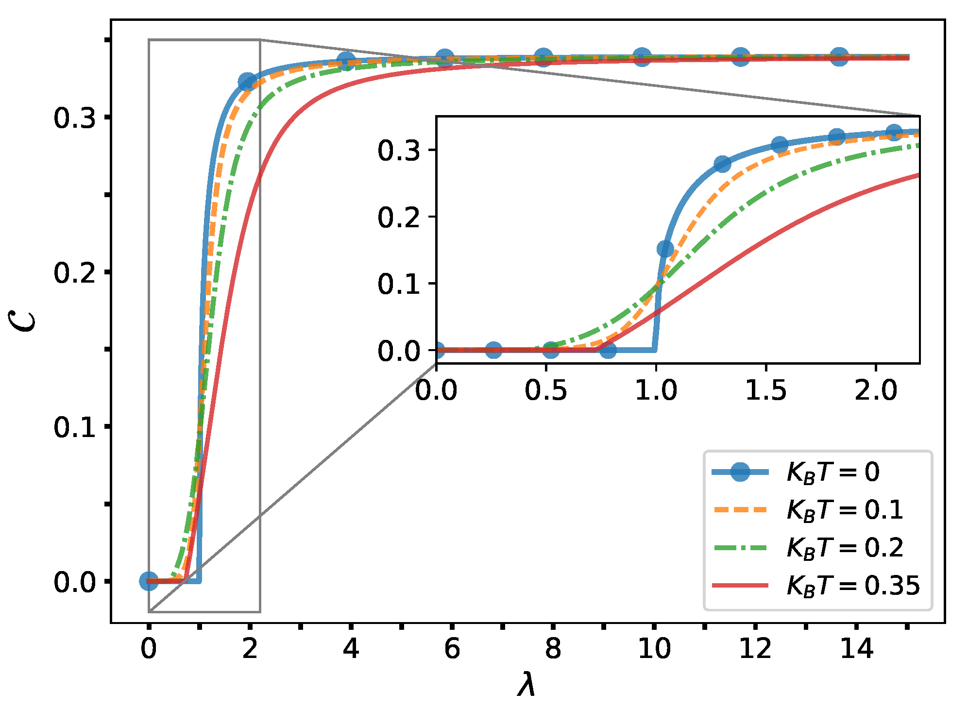
Figure 1. Nearest neighbor concurrence versus λ in the isotropic limit and for magnetic field h = 1 for different values of k B T . The inset amplifies things in the range 0 < λ < 2 .
Quantumrep 02 00020 g001
Figure 2. C x vs. λ for different temperatures. If they are low enough, the site-entanglement emergence at λ 1 is clearly manifested by a C x -peak. Of course, this peak becomes less and less prominent as T grows, and eventually disappears.
Quantumrep 02 00020 g002
Figure 3. Parametric mapping ( C ( λ ) , C x ( λ ) ) for a magnetic field h = 1 ( C ( λ ) is the nearest neighbor concurrence).
Quantumrep 02 00020 g003