Probability Representation of Quantum Mechanics Where System States Are Identified with Probability Distributions ^†

Abstract

The probability representation of quantum mechanics where the system states are identified with fair probability distributions is reviewed for systems with continuous variables (the example of the oscillator) and discrete variables (the example of the qubit). The relation for the evolution of the probability distributions which determine quantum states with the Feynman path integral is found. The time-dependent phase of the wave function is related to the time-dependent probability distribution which determines the density matrix. The formal classical-like random variables associated with quantum observables for qubit systems are considered, and the connection of the statistics of the quantum observables with the classical statistics of the random variables is discussed.

1. Introduction

The goal of this work is to discuss some aspects of the new formulation of quantum mechanics where system states are described by the probability distributions. The Schrödinger and von Neumann equations take the form of kinetic equations for the probability distributions. In the conventional formulation of quantum mechanics, a system state (e.g., the oscillator state) is associated with the wave function [1]. In the presence of interaction of the system with the heat bath, the system state is identified with the density matrix [2,3]. The wave functions and density matrices are associated with state vectors in the Hilbert spaces and density operators acting on the vectors [4]. The physical observables—e.g., the energy of the oscillator—in the conventional formulation of quantum mechanics are described by the Hermitian matrices or Hermitian operators—e.g., the Hamiltonian of the oscillator—acting in the Hilbert space of the system state vectors. The aim of this work is to discuss the probability representation of quantum states—e.g., of the oscillator states [5,6,7,8].

In this representation, the quantum states are identified with fair probability distributions containing the same information on the states, which is contained in the state density operator. In this probability representation of quantum mechanics, physical observables are associated with the sets of formal classical-like random variables. The evolution of the quantum states described in the conventional formulation of quantum mechanics by the Schrödinger equation for the wave function or by the von Neumann equation for the density operator, as well as by the Gorini–Kossakowskii–Sudarshan–Lindblad (GKSL) equation [9,10], is described by the kinetic equations for the probability distributions identified with the quantum states.

The suggested probability representation is constructed using the invertible map of the probability distributions on the density operators acting in the Hilbert space. For example, in the case of systems with continuous variables like the harmonic oscillator, the invertible map is given either by the Radon transform [11] of the state Wigner function [12] or by the fractional Fourier transform of the wave function [13]. The tomographic probability distributions of spin states were discussed in [14,15,16]. We point out that different representations—like the Wigner function representation for the system states with discrete variables based on using the formalism of the quantizer operators—were studied in [17,18,19,20]. Gauge invariance of quantum mechanics in the probability representation was studied in [21].

This paper is organized as follows.

In Section 2, the case of the tomographic probability distribution of a system with continuous variables like the harmonic oscillator is considered. In Section 3, the generic method of quantization, based on using the quantizer–dequantizer operators [22,23] to introduce the associative product (star product) of the symbols of the operators, is discussed. In Section 4, the gauge invariance of the von Neumann equation and the gauge transform of the wave functions (state vectors) are studied. The gauge invariance is used to investigate the phase factor of the state vector depending on time in the probability representation of quantum mechanics. The qubit (spin-1/2) states are described in the probability representation of quantum mechanics in Section 5. Quantum observables are mapped onto the set of formal classical-like random variables in Section 6. The notion of distance between different quantum states is characterized using the standard notion of the difference between the probability distributions in Section 7. In Section 8, the evolution of quantum states is considered in the probability representation and in the other representations using the quantizer–dequantizer formalism. Conclusions are presented in Section 9.

2. Quantum State Description by Probability Distribution for the Case of Continuous Variables

The possibility of describing the states of systems with continuous variables—like the oscillator system—by probability distributions can be demonstrated on an example of the use of tomographic probability distribution [5,6,7]. For the harmonic oscillator state, the symplectic tomographic probability distribution can be introduced using the fractional Fourier transform of the wave function $\langle y|\psi \rangle =\psi (y)$. The function [13]

$$w_{\psi }(X|\mu ,\nu )=\frac{1}{2\pi |\nu |}{\left|\int \psi (y)exp\left(\frac{i\mu }{2\nu }{y}^2-\frac{iX}{\nu }y\right)dy\right|}^2,-\infty \le X,\mu ,\nu <\infty$$

(1)

has the following properties. It is nonnegative and normalized for arbitrary parameters $\mu$ and $\nu$, i.e.,

$$\int w_{\psi }(X|\mu ,\nu )dX=1,$$

(2)

if the wave function is normalized, i.e., ${\displaystyle {\int |\psi (y)|}^{2}dy=1}$.

The density operator ${\widehat{\rho }}_{\psi }=|\psi \rangle \langle \psi |$ of the pure state $|\psi \rangle$ can be reconstructed as follows [7]:

$${\widehat{\rho }}_{\psi }=\frac{1}{2\pi }\int dXd\mu d\nu w_{\psi }(X|\mu ,\nu )exp[i(X-\mu \widehat{q}-\nu \widehat{p})],$$

(3)

where $\widehat{q}$ and $\widehat{p}$ are the position and momentum operators, respectively. For mixed states with the density operator $\widehat{\rho }={\sum }_k{p}_k{\widehat{\rho }}_{{\psi }_k},0\le p_k\le 1,{\sum }_k{p}_k=1$, the probability distribution $w_{\rho }(X|\mu .\nu )$ reconstructs the operator $\widehat{\rho }$ in view of the same Formula (3). For a given operator $\widehat{\rho }$, the tomographic probability distribution, called the symplectic tomogram of the state, is given by the relation [22,23]

$$w_{\rho }(X|\mu ,\nu )=\mathrm{Tr}\widehat{\rho }\delta (X-\nu \widehat{q}-\nu \widehat{p}).$$

(4)

If the real parameters $\mu$ and $\nu$ are described as $\mu =scos\theta$ and $\nu =s^{-1}sin\theta$, where $s=1$, the tomogram coincides with the optical tomogram $w^{\mathrm{opt}}(X|\theta )$ used to measure photon states [24], i.e.,

$$w^{\mathrm{opt}}(X|\theta )=\mathrm{Tr}\widehat{\rho }\delta (X-\widehat{q}cos\theta -\widehat{p}sin\theta ).$$

(5)

Here, $\theta$ is the local oscillator phase and X is the photon quadrature.

The optical tomogram of the pure state is related to the Wigner function [12] of the system via the Radon transform [25,26],

$$w_{\psi }^{\mathrm{opt}}(X|\theta )=\frac{1}{2\pi }\int W_{\psi }(q,p)delta(X-qcos\theta -psin\theta )dqdp,$$

(6)

where

$$W_{\psi }(q,p)=\int \psi (q+u/2){\psi }^{*}(q-u/2)exp(-ipu)du,\frac{1}{2\pi }\int W_{\psi }(q,p)=1.$$

The optical tomogram is related to the symplectic tomogram $w^{\mathrm{opt}}(X|\theta )=w(X|cos\theta ,sin\theta )$. If we know the optical tomogram, the symplectic tomogram is given by the formula

$$w(X|\mu ,\nu )=\frac{1}{\sqrt{{\mu }^2+{\nu }^2}}{w}^{\mathrm{opt}}\left(\frac{X}{\sqrt{{\mu }^2+{\nu }^2}}\left|arctan\left(\frac{\nu }{\mu }\right)\right.\right),$$

(7)

in view of the property of the Dirac delta-function $\delta (\lambda x)={\displaystyle \frac{1}{|\lambda |}}\delta (x)$ used to define the tomogram (4).

The harmonic oscillator states, such as Fock states $|n\rangle ,n=0,1,2,\dots$, are described in the probability representation of quantum mechanics by the distributions $(m=\hslash =\omega =1)$

$$w_n(X|\mu ,\nu )=\frac{exp\left[-X^2/({\mu }^2+{\nu }^2)\right]}{\sqrt{\pi ({\mu }^2+{\nu }^2)}}\frac{1}{2^{n}n!}{H}_n^2\left(\frac{X}{\sqrt{{\mu }^2+{\nu }^2}}\right).$$

(8)

Here, $H_n$ is the Hermite polynomial.

The coherent states $|\alpha \rangle$ [27,28,29], the eigenfunctions of the oscillator annihilation operator $\widehat{a}|\alpha \rangle =\alpha |\alpha \rangle ,\widehat{a}=(\widehat{q}+i\widehat{p})/\sqrt{2}$, are described by the normal distributions

$$w_{\alpha }(X|\mu ,\nu )=\frac{1}{\sqrt{2\pi \sigma (\mu ,\nu )}}exp\left[-\frac{{(X-\overline{X}(\mu ,\nu ))}^2}{2\sigma (\mu ,\nu )}\right],$$

(9)

$$\overline{X}(\mu ,\nu )=\mu \sqrt{2}\mathrm{Re}\alpha +\nu \sqrt{2}\mathrm{Im}\alpha ,\sigma (\mu ,\nu )=\frac{{\mu }^2+{\nu }^2}{2}.$$

(10)

The time evolution of the tomogram of the harmonic oscillator state is determined by the Green function [30], namely,

$$w(X|\mu ,\nu ,t)=\int w(X^{\prime }|{\mu }^{\prime },{\nu }^{\prime },0)G(X,\mu ,\nu ,X^{\prime },{\mu }^{\prime },{\nu }^{\prime },t)d{X}^{\prime }d{\mu }^{\prime }d{\nu }^{\prime },$$

(11)

which can be expressed in terms of the Green function of the Schrödinger equation for the harmonic oscillator

$$g(y,y^{\prime },t)=\frac{1}{\sqrt{2\pi isint}}exp\left(i\frac{y^2+y^{\prime 2}}{2tant}-i\frac{y{y}^{\prime }}{sint}\right).$$

(12)

The above function provides the formula for the evolution of the oscillator’s wave function

$$\psi (y,t)=\int g(y,y^{\prime },t)\psi (y^{\prime },0)d{y}^{\prime }.$$

(13)

Using this formula and relations (1), (3), and (4) for the tomogram expressed in terms of the wave function, we obtain the expression for the Green function in (11). Since the Green function in (13) can be given in the form of the path integral [31,32]

$$g(y,y^{\prime },t)=\int D\left(u(t)\right)exp\left\{i{S}_{\mathrm{cl};y,y^{\prime }}\left(u(t)\right)\right\},$$

(14)

where y and $y^{\prime }$ are the initial and final points of classical trajectories and $S_{\mathrm{cl};y,y^{\prime }}\left(u(t)\right)$ is the classical action, the path integral formulation of quantum mechanics can be also applied in the probability representation of quantum states.

The generic evolution kernel for the tomogram in (11) reads in terms of the path integral as follows:

$$\begin{array}{cc}G(X,\mu ,\nu ,X^{\prime },{\mu }^{\prime },{\nu }^{\prime },t)\hfill & =\frac{1}{2\pi }\int \left[\int D\left(u(t)\right)D\left(v(t)\right)exp\left\{-i{S}_{\mathrm{cl};y,x}\left(u(t)\right)+i{S}_{\mathrm{cl};x^{\prime },y^{\prime }}\left(v(t)\right)\right\}\right]\hfill \\ & \times \langle x|\delta (X^{\prime }-{\mu }^{\prime }\widehat{q}-{\nu }^{\prime }\widehat{p})|x^{\prime }\rangle \langle y^{\prime }|exp\left(i(X-\mu \widehat{q}-\nu \widehat{p})\right)|y\rangle dxdyd{x}^{\prime }d{y}^{\prime }.\hfill \end{array}$$

(15)

Here, the matrix elements of the Weyl operator in the position representation are

$$\langle y^{\prime }|exp\left(i(X-\mu \widehat{q}-\nu \widehat{p})\right)|y\rangle =exp\left(iX+\frac{i\mu \nu }{2}-i\mu y^{\prime }\right)\delta (y^{\prime }-y-\nu ).$$

(16)

The matrix elements of the expression with the Dirac delta-function read

$$\langle x|\delta (X^{\prime }-{\mu }^{\prime }\widehat{q}-{\nu }^{\prime }\widehat{p})|x^{\prime }\rangle =\frac{1}{2\pi |{\nu }^{\prime }|}exp\left\{\frac{i(x-x^{\prime })}{{\nu }^{\prime }}\left[X^{\prime }-{\mu }^{\prime }\frac{x+x^{\prime }}{2}\right]\right\}.$$

(17)

In view of the term in the matrix element of the Weyl operator (16) and the term with the Dirac delta-function in (17), after integrating in (15) over variable $y^{\prime }$, we arrive at the result

$$\begin{array}{c}G(X,\mu ,{\nu }^{\prime },X^{\prime },{\mu }^{\prime },\nu ,t)\hfill \\ =\frac{1}{4{\pi }^2|{\nu }^{\prime }|}\int \left[\int D\left(u(t)\right)D\left(v(t)\right)exp\left\{-i{S}_{\mathrm{cl};y,x}\left(u(t)\right)+i{S}_{\mathrm{cl};x^{\prime },(y+\nu )}\left(v(t)\right)\right\}\right]\hfill \\ \times exp\left\{\frac{i\left(x-x^{\prime }\right)}{{\nu }^{\prime }}\left[X^{\prime }-{\mu }^{\prime }\frac{x+x^{\prime }}{2}\right]\right\}exp\left[i\left(X-\frac{\mu \nu }{2}-\mu y\right)\right]dxdyd{x}^{\prime }.\hfill \end{array}$$

(18)

For the harmonic oscillator, the Green function $g(y,y^{\prime },t)$ (12) is expressed in terms of the path integral ${\displaystyle g(y,y^{\prime },t)=\int D\left(u(t)\right)exp\left[i{S}_{\mathrm{cl};y,y^{\prime }}\left(u(t)\right)\right].}$ Thus, for the harmonic oscillator, we derive the integral expression for the Green function (propagator), which describes the evolution of symplectic tomographic probability distribution as follows:

$$\begin{array}{c}G(X,\mu ,\nu ,X^{\prime },{\mu }^{\prime },{\nu }^{\prime },t)\hfill \\ =\frac{1}{8{\pi }^3|{\nu }^{\prime }|}\int exp\left(-i\frac{y^2+x^2}{2tant}+i\frac{yx}{sint}+i\frac{x^{\prime 2}+{(y+\nu )}^2}{2tant}-i\frac{x^{\prime }(y+\nu )}{sint}\right)\hfill \\ \times exp\left\{\frac{i(x-x^{\prime })}{{\nu }^{\prime }}\left[X^{\prime }-{\mu }^{\prime }\frac{x+x^{\prime }}{2}\right]\right\}exp\left[i\left(X-\frac{\mu \nu }{2}-\mu y\right)\right)dxdyd{x}^{\prime }.\hfill \end{array}$$

(19)

The propagator is expressed in the form of a Gaussian integral, and the result of the integration applied to the initial tomogram provides the same result, which one can obtain using the propagator,

$$G(X,\mu ,\nu ,{\mu }^{\prime },{\nu }^{\prime },t)=\delta (X-X^{\prime })\delta (\mu cost-\nu sint-{\mu }^{\prime })\delta (\nu cost+\mu sint-{\nu }^{\prime }).$$

(20)

3. Quantizer–Dequantizer Formalism

The presented approach is the example of using the formalism of the quantizer–dequantizer method [22,23,33,34] applied for the quantization of classical system states in the tomographic probability representation of quantum mechanics. In this section, we formulate the relation of the path-integral method to the quantizer–dequantizer formalism by providing different representations of the quantum state evolution such as the evolution of the Wigner function [12] and the Glauber–Sudarshan [27,28] and Husimi–Kano [35,36] quasidistributions; for a review, see [37].

For a given Hilbert space $\mathcal{H}$, the sets of two operators $\widehat{\mathcal{U}}(\overrightarrow{\gamma })$ and $\widehat{\mathcal{D}}(\overrightarrow{\gamma })$—where $\widehat{\gamma }=({\gamma }_1,{\gamma }_2,\dots ,{\gamma }_N)$—are continuous or discrete variables, and are called dequantizer and quantizer operators [22,38,39], respectively, if for any operator $\widehat{A},$ one has the equalities

$$f_A(\overrightarrow{\gamma })=\mathrm{Tr}\widehat{A}\widehat{\mathcal{U}}(\overrightarrow{\gamma }),$$

(21)

$$\widehat{A}=\int f_A(\overrightarrow{\gamma })\widehat{\mathcal{D}}(\overrightarrow{\gamma })d\overrightarrow{\gamma }.$$

(22)

The product of the operators $\widehat{A}\widehat{B}$ is mapped onto the associative product of functions $(f_A*f_B)(\overrightarrow{\gamma })$, called the star product. The function $f_A(\overrightarrow{\gamma })$ is called the symbol of the operator $\widehat{A}$. In the considered representation of states, either by means of the Wigner function or by means of symplectic tomographic probability distribution, one uses known dequantizer–quantizer pairs of the operators.

In the case of the Wigner function $\overrightarrow{\gamma }=(q,p)$,

$$\widehat{\mathcal{U}}(q,p)=\int |q+u/2\rangle \langle q-u/2|e^{-ipu}du,$$

(23)

and $\widehat{\mathcal{D}}(q,p)={\displaystyle \frac{1}{2\pi }}\widehat{\mathcal{U}}(q,p)$.

In the case of the symplectic tomographic probability representation, $\overrightarrow{\gamma }=(X,\mu ,\nu )$, and the dequantizer reads

$$\widehat{\mathcal{U}}(X,\mu ,\nu )=\delta (X-\mu \widehat{q}-\nu \widehat{p}).$$

(24)

The quantizer has the form of the Weyl operator

$$\widehat{\mathcal{D}}(X,\mu ,\nu )=\frac{1}{2\pi }exp[i(X-\mu \widehat{q}-\nu \widehat{p})].$$

(25)

Now we present the expression for the propagator of the symbol of the density operator $\widehat{\rho }$ in terms of generic dequantizer–quantizer operators and the path integral which determines the wave function evolution; it is

$$\begin{array}{cc}G(\overrightarrow{\gamma },{\overrightarrow{\gamma }}^{\prime },t)\hfill & =\int \left[\int D\left(u(t)\right)D\left(v(t)\right)exp\left\{-i{S}_{\mathrm{cl};y,x}\left(u(t)\right)+i{S}_{\mathrm{cl};x^{\prime },y^{\prime }}\left(v(t)\right)\right\}\right]\hfill \\ & \times \langle x|\widehat{\mathcal{U}}({\overrightarrow{\gamma }}^{\prime })|x^{\prime }\rangle \langle y^{\prime }|\widehat{\mathcal{D}}(\overrightarrow{\gamma })|y\rangle dxdyd{x}^{\prime }d{y}^{\prime }.\hfill \end{array}$$

(26)

This formula is a generalization of Formula (15) to the case of an arbitrary known representation of quantum states given in the form of expressions containing the dequantizer–quantizer operators. The formulated approach provides the relation of the path integral quantization of the classical mechanics with known star-product schemes of quantization.

4. Gauge Invariance and the Probability Representation of Quantum States

Using the dequantizer–quantizer formalism, gauge invariance in the probability representation of quantum mechanics was considered in [21].

The pure state vector $|\psi \rangle$ of a quantum system [4] satisfies the Schrödinger equation

$$i\frac{\partial |\psi (t)\rangle }{\partial t}=\widehat{H}(t)|\psi (t)\rangle .$$

(27)

Here, we take Planck’s constant ℏ = 1; also, the state vector belongs to the Hilbert space; e.g., the N-dimensional Hilbert space of qudit states. The Hilbert space can be also infinite-dimensional, e.g., for the harmonic oscillator system states. In the generic case, the operator $\widehat{H}(t)$ is the time-dependent operator (Hamiltonian of the system) acting in the Hilbert space of the system states. The density operator of the pure state ${\widehat{\rho }}_{\psi }(t)$, which is determined by the state vector, i.e.,

$${\widehat{\rho }}_{\psi }(t)=|\psi (t)\rangle \langle \psi (t)|,$$

(28)

satisfies the von Neumann evolution equation [3]

$$i\frac{\partial {\widehat{\rho }}_{\psi }(t)}{\partial t}+\left(\widehat{H}(t){\widehat{\rho }}_{\psi }(t)-{\widehat{\rho }}_{\psi }(t)\widehat{H}(t)\right)=0.$$

(29)

The gauge transform of the state vector of the form

$$|\psi (t)\rangle =e^{i\chi (t)}|{\psi }_0(t)\rangle ,$$

(30)

where $\chi (t)$ is the time-dependent phase, is the symmetry transform of the von Neumann equation, since the density operator of the pure state with the state vector $|{\psi }_0(t)\rangle$ is equal to the density operator of the pure state with the state vector $|\psi (t)\rangle$, i.e., ${\widehat{\rho }}_{\psi }(t)={\widehat{\rho }}_{{\psi }_0}(t)$. In view of this fact, the density operator ${\widehat{\rho }}_{{\psi }_0}(t)$ satisfies the same evolution Equation (29). In the case of a mixed state of the system with the density operator given as an arbitrary convex sum of the pure state density operators, i.e.,

$$\widehat{\rho }(t)=\sum _k{\lambda }_k{\widehat{\rho }}_{{\psi }_k}(t),0\le {\lambda }_k\le 1,\sum _k{\lambda }_k=1,$$

(31)

the operator $\widehat{\rho }(t)$ satisfies the evolution Equation (29).

Now we consider the influence of the gauge transform (30) and express the connection of the Schrödinger equations for state vectors $|\psi (t)\rangle$ and $|{\psi }_0(t)\rangle$, using the time dependence of the phase $\chi (t)$. In view of (30), we obtain the evolution equation for the state vector $|{\psi }_0(t)\rangle$ of the form

$$i\frac{{\partial |\psi (t)}_0\rangle }{\partial t}={\widehat{H}}_{\chi }(t)|{\psi }_0(t)\rangle ,$$

(32)

where the Hamiltonian ${\widehat{H}}_{\chi }(t)$ reads

$${\widehat{H}}_{\chi }(t)=[\widehat{H}(t)+\dot{\chi }(t)\widehat{1}].$$

(33)

The unitary evolution operator $\widehat{U}(t)$, which describes the evolution of the state vector $|\psi (t)\rangle$, namely,

$$|\psi (t)\rangle =\widehat{U}(t)|\psi (t=0)\rangle ,$$

(34)

satisfies the equation

$$i\frac{\partial \widehat{U}(t)}{\partial t}=\widehat{H}(t)\widehat{U}(t)$$

(35)

with the initial condition $\widehat{U}(t=0)=\widehat{1}$.

In the case of the qubit, for the time-independent Hamiltonian

$$H=\left(\begin{array}{cc}{H}_{11}& H_{12}\\ H_{12}^{*}& H_{22}\end{array}\right),$$

(36)

the unitary matrix $U(t)$ reads

$$U(t)=exp\left[-it\left(\begin{array}{cc}{H}_{11}& H_{12}\\ H_{12}^{*}& H_{22}\end{array}\right)\right]=exp\left(-\frac{it}{2}(H_{11}+H_{22})\right)M(t),$$

(37)

where the unitary matrix $M(t)$ is

$$M(t)=\left(\begin{array}{cc}cos\mathsf{\Omega }t-{\displaystyle \frac{isin\mathsf{\Omega }t}{2\mathsf{\Omega }}}(H_{11}-H_{22})& -{\displaystyle \frac{isin\mathsf{\Omega }t}{\mathsf{\Omega }}}{H}_{12}\\ -{\displaystyle \frac{isin\mathsf{\Omega }t}{\mathsf{\Omega }}}{H}_{12}^{*}& cos\mathsf{\Omega }t+{\displaystyle \frac{isin\mathsf{\Omega }t}{2\mathsf{\Omega }}}(H_{22}-H_{11})\end{array}\right).$$

(38)

Here, the frequency $\mathsf{\Omega }$ is given by formula

$$\mathsf{\Omega }=\sqrt{H_{12}{H}_{12}^{*}+{\left[(H_{11}-H_{22})/2\right]}^2}.$$

(39)

Analogously, the evolution of the state vector $|{\psi }_0(t)\rangle$ is described by the unitary operator $U_{\chi }(t)$, which satisfies Equation (35), where the Hamiltonian $\widehat{H}(t)$ is replaced by the operator $(\widehat{H}(t)+\dot{\chi }(t)\widehat{1})$. The unitary evolution operators $\widehat{U}(t)$ and ${\widehat{U}}_{\chi }(t)$ are different ones but, due to the gauge invariance of the von Neumann equation for the density operators satisfying Equation (29) with Hamiltonians $\widehat{H}(t)$ and ${\widehat{H}}_{\chi }(t)$, the density operators are equal. In the case of continuous variables, the wave function $\psi (x,t)=\langle x|\psi (t)\rangle$ and the function ${\psi }_0(x,t)=\langle x|{\psi }_0(t)\rangle$ are different. The Schrödinger equation for the system wave function $\psi (x,t)$, written in the form of an equation for the function ${\psi }_0(x,t)$ following from Equation (32) for the vector $|{\psi }_0(t)\rangle$, provides the relation

$$\dot{\chi }(t)=i\frac{\partial }{\partial t}ln{\psi }_0(x,t)-{\psi }_0^{-1}(x,t)\widehat{H}(t){\psi }_0(x,t).$$

(40)

This relation contains information on the phase $\chi (t)$, determining the gauge transform of the wave function $\psi (x,t)$, which does not change the density matrix

$${\rho }_{\psi }(x,x^{\prime },t)=\langle x|\psi (t)\rangle \langle \psi (t)|x^{\prime }\rangle ={\rho }_{{\psi }_0}(x,x^{\prime },t)=\langle x|{\psi }_0(t)\rangle \langle {\psi }_0(t)|x^{\prime }\rangle .$$

Analogous consideration can be presented in the case of N-dimensional Hilbert space, e.g., in the case of a qubit system with $N=2$.

5. Qubit State in the Probability Representation

In the case of qubits (two-level atom, spin-1/2 system), the variable x takes two values $x\to m=\pm 1/2$, where m is the spin-1/2 projection in the z-direction. The pure state is described by the state vector $|\psi \rangle$ with two components $|\psi \rangle =\left(\begin{array}{c}{\psi }_{+1/2}\\ {\psi }_{-1/2}\end{array}\right)$ satisfying the normalization condition $\langle \psi |\psi \rangle =|{\psi }_{+1/2}{|}^2+{|{\psi }_{-1/2}|}^2=1$. The $2\times 2$ density matrix of the pure state ${\rho }_{\psi }$ reads

$${\rho }_{\psi }=\left(\begin{array}{cc}|{\psi }_{+1/2}{|}^2& {\psi }_{+1/2}{\psi }_{-1/2}^{*}\\ {\psi }_{-1/2}{\psi }_{+1/2}^{*}& |{\psi }_{-1/2}{|}^2\end{array}\right).$$

(41)

The $2\times 2$ density matrix ${\rho }_{m{m}^{\prime }}$ of the mixed state has the matrix elements expressed in terms of probabilities $p_1,p_2,p_3$ [40,41]:

$$\rho =\left(\begin{array}{cc}{p}_3& (p_1-1/2)-i(p_2-1/2)\\ (p_1-1/2)+i(p_2-1/2)& 1-p_3\end{array}\right).$$

(42)

Here, the numbers $0\le p_1,p_2,p_3\le 1$ determine three probability distributions—$(p_1,1-p_1)$, $(p_2,1-p_2)$, and $(p_3,1-p_3)$—of dichotomic random variables. These numbers satisfy the Silvester criterion of nonnegativity of the matrix eigenvalues:

$$\sum _{j=1}^N{\left(p_j-1/2\right)}^2\le 1/4.$$

(43)

For the pure state with the density matrix given by (41) satisfying the condition ${\rho }_{\psi }^2={\rho }_{\psi }$, we have equality ${\sum }_{j=1}^N{\left(p_j-1/2\right)}^2=1/4.$ Our aim is to consider the gauge invariance property of matrix (42). We introduce vector $|{\psi }_0(t)\rangle$ of the form

$$|{\psi }_0(t)\rangle =\left(\begin{array}{c}\sqrt{p_3(t)}\\ {\displaystyle \frac{1}{\sqrt{p_3(t)}}}\left[(p_1(t)-1/2)+i(p_2(t)-1/2)\right]\end{array}\right).$$

(44)

The vector $|\psi (t)\rangle =e^{i\chi (t)}|{\psi }_0(t)\rangle$ gives the density matrix of the form (42). Equation (40) provides the relation of the phase $\chi (t)$ to probabilities $p_1(t)$, $p_2(t)$, and $p_3(t)$. In fact, the probabilities satisfy the von Neumann evolution equation for the density matrix $|{\psi }_0(t)\rangle \langle {\psi }_0(t)|$ of the form

$$\begin{array}{c}\left(\begin{array}{cc}{\displaystyle \frac{d}{dt}}{p}_3(t)& {\displaystyle \frac{d}{dt}}{p}_1(t)-i{\displaystyle \frac{d}{dt}}{p}_2(t)\\ {\displaystyle \frac{d}{dt}}{p}_1(t)+i{\displaystyle \frac{d}{dt}}{p}_2(t)& -{\displaystyle \frac{d}{dt}}{p}_3(t)\end{array}\right)\hfill \\ =\left(\begin{array}{cc}{H}_{11}(t)& H_{12}(t)\\ H_{21}(t)& H_{22}(t)\end{array}\right)\left(\begin{array}{cc}{p}_3(t)& (p_1(t)-1/2)-i(p_2(t)-1/2)\\ (p_1(t)-1/2)+i(p_2(t)-1/2)& 1-p_3(t)\end{array}\right)\hfill \\ -\left(\begin{array}{cc}{p}_3(t)& (p_1(t)-1/2)-i(p_2(t)-1/2)\\ (p_1(t)-1/2)+i(p_2(t)-1/2)& 1-p_3(t)\end{array}\right)\left(\begin{array}{cc}{H}_{11}(t)& H_{12}(t)\\ H_{21}(t)& H_{22}(t)\end{array}\right).\hfill \end{array}$$

(45)

This matrix equation provides the connection of the time derivatives ${\displaystyle \frac{d{p}_j(t)}{dt}}$; $j=1,2,3$ with probabilities and matrix elements of the Hamiltonian $H_{jk}(t);$ $j,k=1,2$. In addition, Equation (40) written for probabilities $p_j(t)$; $j=1,2,3$ takes the form

$$i\frac{d}{dt}\sqrt{p_3(t)}=\left[H_{11}(t)+\dot{\chi }(t)\right]\sqrt{p_3(t)}+H_{12}(t)\frac{(p_1(t)-1/2)+i(p_2(t)-1/2)}{\sqrt{p_3(t)}}.$$

(46)

Thus, using (40), we can obtain the connection of the phase $\chi (t)$ with probabilities $p_1(t)$, $p_2(t)$, and $p_3(t)$. For the case of the spin-1/2 pure state with matrix elements of the Hamiltonian $H_{jk}$; $j=1,2,$ one obtains the evolution equation for the phase $\chi (t)$ of the Pauli spinor of the form

$$\frac{d\chi (t)}{dt}=p_3^{-1}(t)\left[(p_2(t)-1/2)\mathrm{Im}{H}_{12}(t)-(p_1(t)-1/2)\mathrm{Re}{H}_{12}(t)\right]-H_{11}(t).$$

(47)

The probabilities $p_1(t)$, $p_2(t)$, and $p_3(t)$ are given as solutions of the kinetic Equation (45), which follows from the von Neumann equation for the density matrix $\rho (t)$ of spin-1/2 states, and it does not contain the phase $\chi (t)$. The evolution Equation (47) can be rewritten using Bloch parameters $B_j(t)=2p_j(t)-1$. These parameters have the physical meaning connected with mean values of the spin-1/2 projections onto three perpendicular directions—x, y, and z, respectively. The equation has the form

$$\frac{d\chi (t)}{dt}={[B_3(t)+1]}^{-1}\left[B_2(t)\mathrm{Im}{H}_{12}(t)-B_1(t)\mathrm{Re}{H}_{12}(t)\right]-H_{11}(t).$$

(48)

The values $B_j(t)$ and probabilities $p_j(t)$ can be measured. This means that one can find the evolution of the phase $\chi (t)$ of the spin-1/2 wave function given by the formula

$$\chi (t)={\int }_0^{t}d\tau \left\{p_3^{-1}(\tau )\left[(p_2(\tau )-1/2)\mathrm{Im}{H}_{12}(\tau )-(p_1(\tau )-1/2)\mathrm{Re}{H}_{12}(\tau )\right]-H_{11}(\tau )\right\},\chi (0)=0.$$

(49)

For the Hamiltonian describing the evolution of the spin-1/2 particle with magnetic moment $\overrightarrow{\mathcal{M}}$ in a constant magnetic field $\overrightarrow{\mathcal{H}}=(0,0,\mathcal{H})$, i.e., $H(t)=-\mathcal{M}\mathcal{H}{\sigma }_z$, the probabilities $p_1(t)$, $p_2(t)$, and $p_3(t)$ depend on the initial values of the state, $p_1(0)$, $p_2(0)$, and $p_3(0)$. For example, if $p_1(0)=p_2(0)=1/2$ and $p_3(0)=1$, one has Equation (47) of the form

$$\frac{d\chi (t)}{dt}=\mathcal{M}\mathcal{H}.$$

(50)

The solution (49) of this equation gives the phase

$$\chi (t)=\mathcal{M}\mathcal{H}t,$$

(51)

and this phase corresponds to the solution of the Schrödinger equation for the Pauli spinor $|\psi (t)\rangle$,

$$|\psi (t)\rangle =\left(\begin{array}{cc}{e}^{-i\mu \mathcal{H}t}& 0\\ 0& e^{i\mu \mathcal{H}t}\end{array}\right)\left(\begin{array}{c}1\\ 0\end{array}\right),$$

(52)

where the initial value $|\psi (0)\rangle$ corresponds to the pure state density matrix $\rho (0)=\left(\begin{array}{cc}1& 0\\ 0& 0\end{array}\right)$, and the initial phase $\chi (0)=0$.

The density matrix $\rho (t)$ corresponding to the pure state (52) does not depend on the magnetic field $\mathcal{H}$ due to the stationarity of probabilities $p_1(t)=p_2(t)=1/2$ and $p_3(t)=1$ in this particular case. However, in the case of the initial state with density matrix $\rho (0)={\displaystyle \frac{1}{2}}\left(\begin{array}{cc}1& 1\\ 1& 1\end{array}\right)$ and $|\psi (0)\rangle ={\displaystyle \frac{1}{\sqrt{2}}}\left(\begin{array}{c}1\\ 1\end{array}\right)$, one has the evolution of probabilities

$$p_1(t)=\frac{1+cos(2\mathcal{M}\mathcal{H}t)}{2},p_2(t)=\frac{1+2sin(2\mathcal{M}\mathcal{H}t)}{2},p_3(t)=\frac{1}{2}.$$

(53)

The phase $\chi (t)$ given by (49) takes into account the connection of the probabilities of the spin-1/2 projections $m=+1/2$ onto perpendicular directions x and y on the magnetic field. Thus, the value of the magnetic field can be found measuring the probability evolution.

6. The Quantum Observable as a Set of Dichotomic Random Variables

As we found, the density matrix of a spin-1/2 system (42) is expressed in terms of three probability distributions, $(p_1,1-p_1)$, ($p_2,1-p_2)$, and $(p_3,1-p_3)$, where the probabilities $p_j,j=1,2,3$ satisfy inequality (43). For an observable

$$A=\left(\begin{array}{cc}{A}_{11}& A_{12}\\ A_{21}& A_{22}\end{array}\right),$$

(54)

one can determine the set of formal classical-like random variables using the following rule.

Let us determine a random dichotomic variable $\overrightarrow{x}$ taking two values, $(x_1=x,x_2=-x)$, and another random variable $\overrightarrow{y}$ taking two values, $(y_1=y,y_2=-y)$, where $x+iy=A_{12}$. The third random variable $\overrightarrow{z}$ takes two real values, $(z_1=A_{11},z_2=A_{22}).$ The introduced random dichotomic variables can be interpreted as the rules in such a game as tossing three classical coins. The game with the first coin has a gain equal to x and a loss equal to $-x$. For the second coin, the gain is equal to y and the loss is equal to $-y$. For the third coin, the gain and loss are not equal; they are denoted as $z_1$ and $z_2$, respectively. We interpret the probability distributions $(p_1,1-p_1)$, $(p_2,1-p_2)$, and $(p_3,1-p_3)$ as distributions describing the classical statistics of random variables $\overrightarrow{x}$, $\overrightarrow{y}$, and $\overrightarrow{z}$. This means that we define the moments for the dichotomic variables

$$\begin{array}{ccc}{M}_n(\overrightarrow{x})=x_1^n{p}_1+(1-p_1)x_2^n,\hfill & \hfill M_n(\overrightarrow{y})=y_1^n{p}_2+(1-p_2)y_2^n,& \hfill M_n(\overrightarrow{z})=z_1^n{p}_3+(1-p_3)z_2^n,\\ & & \hfill n=1,2,\dots \end{array}$$

(55)

The quantum statistics of observable (54) are described by the matrix A and the density matrix $\rho$ given by (42) as follows:

$$\langle A^n\rangle =\mathrm{Tr}\rho A^n,n=1,2,\dots$$

(56)

One can check that, for the quantum observable A, the mean value $\langle A\rangle$ is expressed in terms of classical mean values $M_1(\overrightarrow{x})$, $M_1(\overrightarrow{y})$, and $M_1(\overrightarrow{z})$, namely,

$$\langle A\rangle =M_1(\overrightarrow{x})+M_1(\overrightarrow{y})+M_1(\overrightarrow{z}).$$

(57)

The highest moments (55) of classical-like random variables, which we used to interpret the matrix elements of the quantum observable A and the quantum moments, e.g., $\langle A^2\rangle$, are not expressed in the form of a sum analogous to (57).

We consider now an example of the qubit thermal equilibrium state with the density matrix $\rho (T)$. For a given Hamiltonian H (36) with matrix elements $H_{jk}$; $j,k=1,2$, the density matrix reads

$$\rho (\beta )=\frac{1}{Z(\beta )}exp(-\beta H),\beta =\frac{1}{T}.$$

(58)

Using the properties of Pauli matrices ${\sigma }_1=\left(\begin{array}{cc}0& 1\\ 1& 0\end{array}\right)$, ${\sigma }_2=\left(\begin{array}{cc}0& -i\\ i& 0\end{array}\right)$, and ${\sigma }_3=\left(\begin{array}{cc}1& 0\\ 0& -1\end{array}\right)$, namely, ${\sigma }_j^2=1$, $\mathrm{Tr}{\sigma }_j=0$; $j=1,2,3$ and the relation $exp\tau (\overrightarrow{\sigma }\overrightarrow{n})=(cosh\tau )1_2+(sinh\tau )\overrightarrow{\sigma }\overrightarrow{n},$ where ${\overrightarrow{n}}^2=1$, we arrive at

$$exp\left(\begin{array}{cc}a& b\\ c& d\end{array}\right)=e^{(a+d)/2}\left(\begin{array}{cc}cosh\tau +{\displaystyle \frac{a-d}{2\tau }}sinh\tau & b{\displaystyle \frac{sinh\tau }{\tau }}\\ c{\displaystyle \frac{sinh\tau }{\tau }}& cosh\tau +{\displaystyle \frac{d-a}{2\tau }}sinh\tau \end{array}\right),$$

(59)

where

$$\tau =\sqrt{{\left[(a-d)/2\right]}^2+bc}$$

(60)

and

$$\mathrm{Tr}\left[exp\left(\begin{array}{cc}q& b\\ c& d\end{array}\right)\right]=2exp\left[(a+d)/2\right]cosh\tau .$$

(61)

The thermal equilibrium state of the qubit at the temperature $T=1/\beta$ is identified with three probabilities, $p_1(\beta )$, $p_2(\beta )$, and $p_3(\beta )$. For Hamiltonian (36), $-\beta H_{11}=a$, $-\beta H_{12}=b$, $-\beta H_{21}=c$, and $-\beta H_{22}=d$, the probabilities read

$$\begin{array}{c}{p}_1(\beta )=\frac{1}{2}\left[1+\frac{(Re{H}_{12})tanh\left(\beta \sqrt{{\left[(H_{11}-H_{22})/2\right]}^2+{|H_{12}|}^2}\right)}{\sqrt{{\left[(H_{11}-H_{22})/2\right]}^2+{|H_{12}|}^2}}\right],\hfill \\ p_2(\beta )=\frac{1}{2}\left[1+\frac{(Im{H}_{12})tanh\left(\beta \sqrt{{\left[(H_{11}-H_{22})/2\right]}^2+{|H_{12}|}^2}\right)}{\sqrt{{\left[(H_{11}-H_{22})/2\right]}^2+{|H_{12}|}^2}}\right],\hfill \\ p_3(\beta )=\frac{1}{2}\left[1+\frac{\left(H_{22}-H_{11}\right)tanh\left(\beta \sqrt{{\left[(H_{11}-H_{22})/2\right]}^2+{|H_{12}|}^2}\right)}{\sqrt{{\left(H_{11}-H_{22}\right)}^2+4{|H_{12}|}^2}}\right].\hfill \end{array}$$

(62)

We arrive at the function $Z(\beta )=\mathrm{Tr}[exp(-\beta H)]$ of the form

$$Z(\beta )=2\left[exp\left(-\beta \left[(H_{11}+H_{22})/2\right]\right)\right]cosh\left(\beta \sqrt{{\left[(H_{11}-H_{22})/2\right]}^2+{|H_{12}|}^2}\right).$$

Thus, the three probabilities $p_j(\beta )$; $j=1,2,3$ describe the statistical properties of thermal equilibrium states of qubits (two-level atoms).

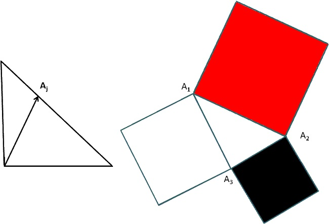
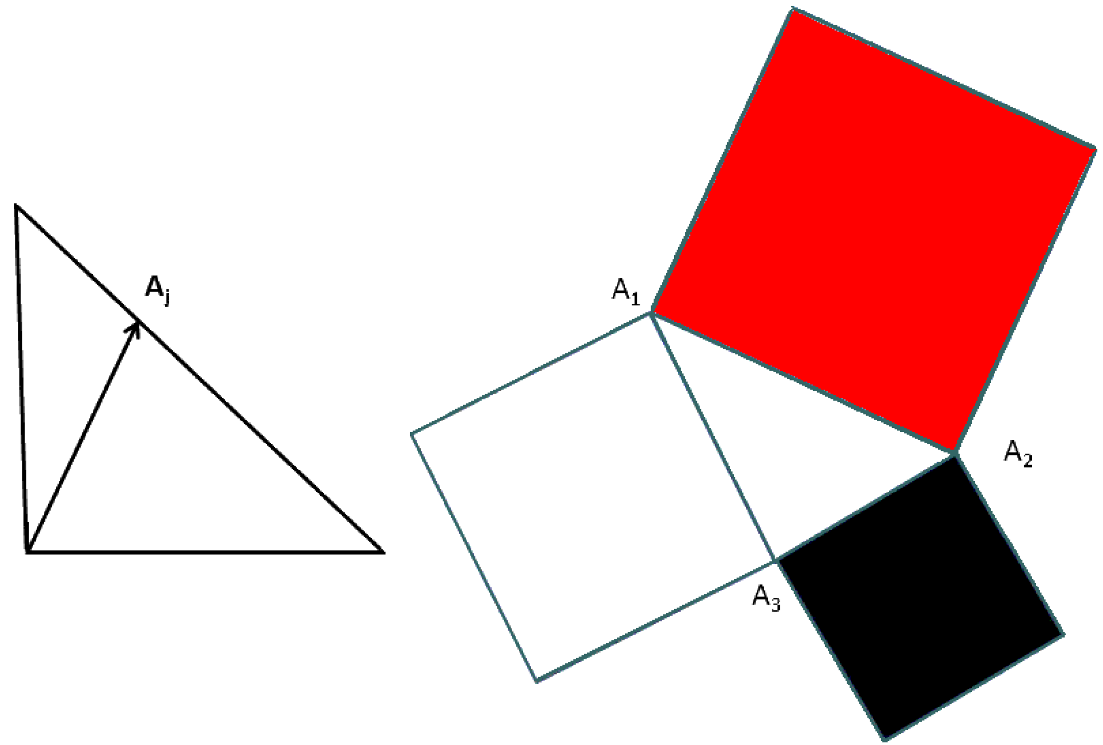
The geometrical picture for all of the states of the qubit is given in terms of Bloch ball parameters. However, the states of the qubit could also be presented in the form of Triada of Malevich’s squares (Figure 1) using the probabilities $p_1$, $p_2$, and $p_3$ [40,42,43].

An equilateral triangle with a side length of $\sqrt{2}$ is given. This triangle is constructed by gluing vertices on hypotenuses of three rectangular triangles with equal legs and with the points $A_j$; $j=1,2,3$. The points have coordinates $p_j$ and $1-p_j$. Inside this equilateral triangle, we have the triangle $A_1{A}_2{A}_3$ with three side lengths:

$$\begin{array}{c}{S}_1={\left(2+2p_1^2-4p_1-2p_2+2p_2^2+2p_1{p}_2\right)}^{1/2},\hfill \\ S_2={\left(2+2p_2^2-4p_2-2p_3+2p_3^2+2p_2{p}_3\right)}^{1/2},\hfill \\ S_3={\left(2+2p_3^2-4p_3-2p_1+2p_1^2+2p_3{p}_1\right)}^{1/2}.\hfill \end{array}$$

(63)

We construct the squares on sides $A_1{A}_2$, $A_2{A}_3$, and $A_3{A}_1$ of triangle $A_1{A}_2{A}_3$. We paint the squares in different colors: The square with side $A_1{A}_2$ is red, the square with side $A_2{A}_3$ is black, and the square with side $A_3{A}_1$ is white. Thus, the state with density matrix $\rho$ can be geometrically described either by the point in the Bloch ball or by the three squares on the plane, called the Triada of Malevich’s squares. This approach was called quantum suprematism [40,42,43].

The quantum nature of the qubit state provides a difference with classical coins, which are also described by the probabilities $p_1$, $p_2$, and $p_3$. The maximum area of the Triada of Malevich’s squares for three classical coins is equal to 6. However, for the qubit state (spin-1/2 state, two-level atom state), it is equal to 3. By measuring Bloch parameters or probabilities $p_1$, $p_2$, and $p_3$, one provides the possibility of checking this property. This measurement is analogous to checking the Bell inequality for a two spin-1/2 system, where the maximum value of specific correlations is equal to $2\sqrt{2}$. The classical-like maximum is equal to 2. However, in the case of the possible measurement of the Malevich’s square areas (i.e., measuring probabilities $p_1$, $p_2$, and $p_3$), the system under investigation is a single spin-1/2 particle. In the case of the Bell inequality, the system under study is the two-qubit system. Thus, one can check the differences in the properties of classical and quantum correlations in the case of one spin-1/2 particle by measuring probabilities $p_1$, $p_2$, and $p_3$, which determine the area of Malevich’s squares.

7. Distance between Quantum States

The probability representation of quantum states can be used to introduce classical-like characteristics of difference between the states in addition to the fidelity. We consider qubit states as an example. For density matrices ${\rho }_1$ and ${\rho }_2$, there exist six probability distributions

$$(p_1^{(1)},1-p_1^{(1)}),(p_2^{(1)},1-p_2^{(1)}),(p_3^{(1)},1-p_3^{(1)}),(p_1^{(2)},1-p_1^{(2)}),(p_2^{(2)},1-p_2^{(2)}),(p_3^{(2)},1-p_3^{(2)})$$

which determine the density matrices. In conventional probability theory, the difference between the two probability distributions $(P_1,P_2,\dots ,P_N)$ and $(Q_1,Q_1,\dots ,Q_N)$ is characterized by the distance parameter

$$S=[{(P_1-Q_1)}^2+{(P_2+Q_2)}^2+\cdots +{(P_N-Q_N)}^2].$$

This classical formula can be used to characterize the difference of quantum states with density matrices ${\rho }_1$ and ${\rho }_2$. We determine such characteristics for the two qubit states as follows:

$$S_{12}=2\sum _{j=1}^3{(p_j^{(1)}-p_j^{(2)})}^2.$$

(64)

In the case of continuous variables, the difference of the two states is characterized by an analogous relation; it reads

$$S_{12}(\mu ,\nu )=\int {\left[w_1(X|\mu ,\nu )-w_2(X|\mu ,\nu )\right]}^{2}dX,$$

(65)

where we use the tomographic probability distributions $w_{1,2}(X|\mu ,\nu )$ corresponding to the states, e.g., of the oscillator with density operators ${\rho }_1$ and ${\rho }_2$, respectively. The difference of the two states depends on the parameters $\mu$ and $\nu$, which describe the reference frames in the phase space where the position X is measured.

In the case of the classical oscillator, for which the tomographic probability distribution can be introduced [6] and expressed in terms of the Radon transform of the classical probability density function $f(q,p)$

$$w_{\mathrm{cl}}(X|\mu ,\nu )=\int f(q,p)\delta (X-\mu q-\nu p)dqdp,$$

(66)

the parameters $\mu =scos\theta$ and $\nu =s^{-1}sin\theta$ correspond to scale and rotation transforms of the position and momentum: $q\to q^{\prime }=sq$, $p\to p^{\prime }=s^{-1}p$, $q^{\prime }\to q^{\prime \prime }=q^{\prime }cos\theta +p^{\prime }sin\theta ,$ and $p^{\prime }\to p^{\prime \prime }=p^{\prime }cos\theta -q^{\prime }sin\theta$, respectively. Thus, we can use the notion of the difference of the states both in classical and quantum mechanics using the tomographic probability distributions.

In connection with the construction of the probability distributions identified with quantum states, one can apply other characteristics of the state difference used in classical probability theory to study the difference of two probability distributions. For example, in addition to (66), the Shannon relative entropy can be considered as a tool to characterize the difference of the two states of photons with two different tomographic probability distributions.

The relative entropy for quantum symplectic and optical tomograms must be nonnegative; i.e., for the symplectic tomogram, we have

$$H_{\mathrm{relative}}=\int w_1(X|\mu ,\nu )ln\left[\frac{w_1(X|\mu ,\nu )}{w_2(X|{\mu }^{\prime },{\nu }^{\prime })}\right]dX\ge 0.$$

This relative entropy can be equal to zero only for equal probability distributions. Since optical tomograms of photon states are measured experimentally [24], tomograms $w_1(X|{\theta }_1)$ and $w_2(X|{\theta }_2)$ must satisfy the inequality for the relative entropy:

$$H({\theta }_1,{\theta }_2)=\int w_1(X|{\theta }_1)ln\left[\frac{w_1(X|{\theta }_1)}{w_2(X|{\theta }_2)}\right]dX\ge 0.$$

This inequality can be checked experimentally. An analogous entropic inequality can be checked for qubit states, namely,

$$\sum _{j=1}^3\left[p_{j}ln\left(\frac{p_j}{{\mathcal{P}}_j}\right)+(1-p_j)ln\left(\frac{1-p_j}{1-{\mathcal{P}}_j}\right)\right]\ge 0,$$

where $p_1,p_2,p_3,{\mathcal{P}}_1,{\mathcal{P}}_2$, and ${\mathcal{P}}_3$ are different probabilities of spin projections $m=+1/2$ on the $x,y,z$-directions in two different spin-$1/2$ states identified with the probability distributions.

For composite systems like that of the two qubits, quantum correlations between the subsystem degrees of freedom can be associated with the probability distributions and their entropies by describing the states of the system and its subsystems. This problem needs extra consideration.

8. The Evolution Equation in the Probability Representation

Given an arbitrary pair of dequantizer–quantizer operators $\widehat{\mathcal{U}}(\gamma )$ and $\widehat{\mathcal{D}}(\gamma )$, the von Neumann Equation (27) can be written for the symbol of operator $\widehat{\rho }(t)$ determined by the dequantizer operator,

$$f_{\rho }(\overrightarrow{\gamma },t)=\mathrm{Tr}\left(\widehat{\mathcal{U}}(\overrightarrow{\gamma })\widehat{\rho }(t)\right);$$

(67)

the equation has the form

$$\frac{\partial }{\partial t}{f}_{\rho }(\overrightarrow{\gamma },t)=\int f_{\rho }({\overrightarrow{\gamma }}^{\prime },t)K(\overrightarrow{\gamma },{\overrightarrow{\gamma }}^{\prime },t)d{\overrightarrow{\gamma }}^{\prime }.$$

(68)

Here, the integral kernel is determined by the quantizer–dequantizer operators [21]

$$K(\overrightarrow{\gamma },{\overrightarrow{\gamma }}^{\prime },t)=i\mathrm{Tr}\left[\widehat{\mathcal{U}}(\overrightarrow{\gamma })\left(\widehat{\mathcal{D}}({\overrightarrow{\gamma }}^{\prime })\widehat{H}-\widehat{H}\widehat{\mathcal{D}}({\overrightarrow{\gamma }}^{\prime })\right)\right].$$

(69)

In the case where the symbol of the density operator is a probability distribution, e.g., in the case of $\overrightarrow{\gamma }=(X,\mu ,\nu )$, using dequantizer–quantizer operators (24) and (25), we arrive at the von Neumann equation of the form of a kinetic equation for tomographic probability distribution $w(X|\mu ,\nu ,t)$ [5]. Equations (68) and (69) provide the unitary evolution description for all known representations of quantum states in the literature, including the probability representation. For optical tomographic probability distribution, the evolution equation was found in [44].

9. Conclusions

To conclude, we point out the main results of our work.

We reviewed the probability representation of quantum states and considered the application of this approach on the examples of harmonic oscillator states and qubit states. In the case of systems with continuous variables, like the harmonic oscillator, we obtained the relation of the probability representation of quantum states with the path integral method. We expressed the propagator describing the evolution of the tomographic probability distribution identified with the quantum state of the system with continuous variables, like the oscillator, with the path integral determining the Green function of the Schrödinger evolution equation for the wave function of the system.

In the generic case of systems with continuous variables, we formulated the connection of the path integral representation of the quantum-state evolution with other representations of quantum states, using the quantizer–dequantizer approach to the quantization of classical systems studied in [22,23,38,39]. The notion of classical-like difference of quantum states was introduced, using the standard notion of the difference of two probability distributions for both the oscillator system and qubit system, where the state is identified with three probability distributions of dichotomic random variables.

We found the equation for the time-dependent phase determining the gauge transform of the wave function. For the qubit state, the equation is given in the form of a relation, where the time-dependent phase is expressed in terms of the probabilities of dichotomic random variables determining the evolution of the density matrix satisfying the von Neumann equation with a given Hamiltonian.

The statistical properties of qubit quantum observables were discussed in relation with the classical statistical properties of the classical-like dichotomic random variables. The different aspects of the relation of the probability theory with properties of quantum or quantum-like states were discussed in [45,46,47,48,49]. We will consider other examples of the connection of the path integral with star-product schemes and entropic inequalities for quantum systems based on the probability representation of quantum mechanics in future publications.