Nonclassical States for Non-Hermitian Hamiltonians with the Oscillator Spectrum


Abstract
1. Introduction
2. Non-Hermitian Oscillators
- Fundamental solutions. Another remarkable profile of the complex-valued oscillators of Equation (3) is that the functionsare normalizable solutions of the related eigenvalue equation for . The additional normalizable functionalso solves the eigenvalue equation defined by , but it is not derivable from the set and belongs to the energy . The spectrum of the potential is therefore composed of the equidistant energies , .
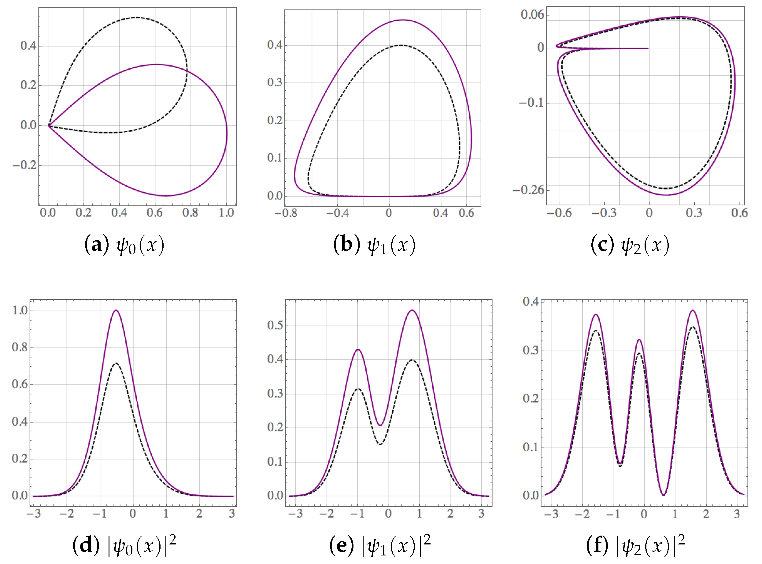
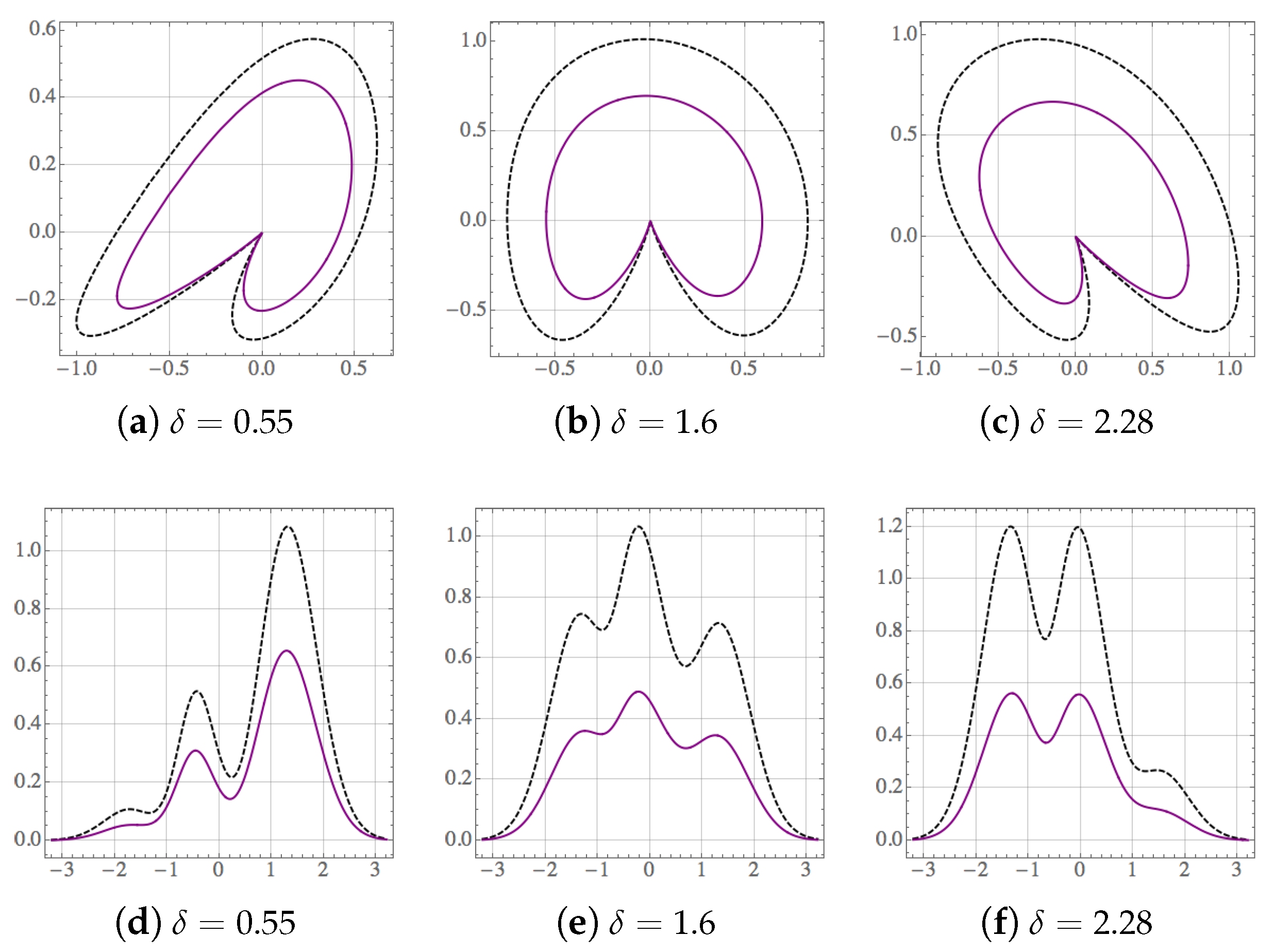
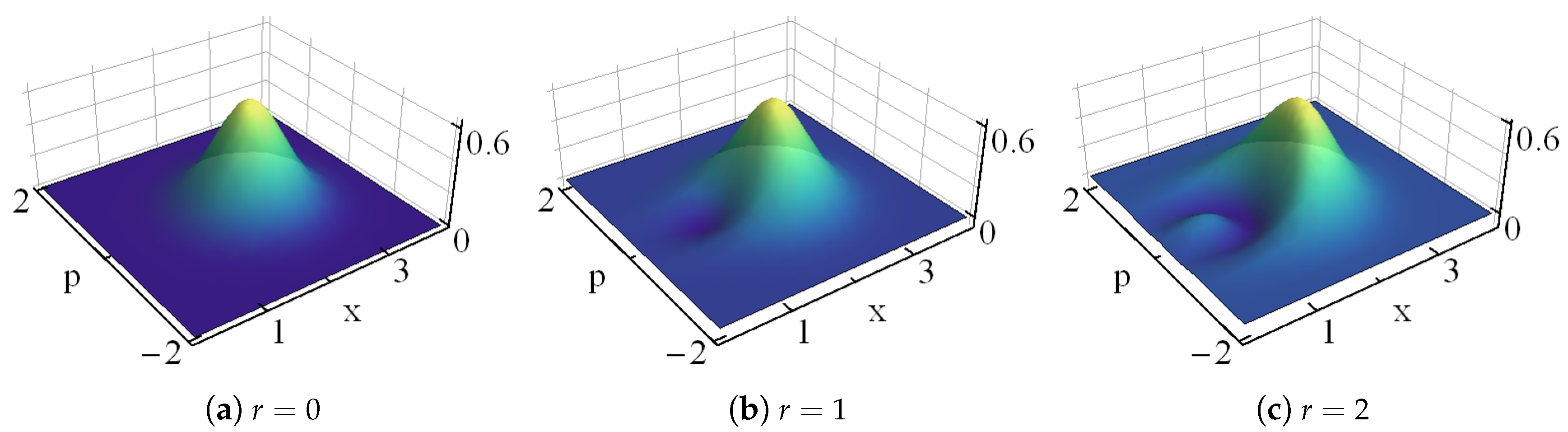
- Bi-orthogonality. While the functions are normalizable, they form a peculiar set since is orthogonal to all the while the latter are not mutually orthogonal. As a result, in contrast with the Hermitian case, the norm of any superposition of states depends not only on the modulus of the related coefficients but also on the phase shift between them. For instance, the norm ofsatisfieswhere is the complex-conjugate of . The numbers and are, respectively, the modulus and argument of the product between and . Thus, depending on the phase-shift , the non-orthogonality of the set produces the oscillations of . The complexity of such a dependence increases with the number of elements in the superposition.One can face the above difficulties by introducing a bi-orthogonal system (see relevant information in Reference [24]), formed by the eigenfunctions of and those of its Hermitian-conjugate , written as . The main point is that the bi-product is equal to zero if , and serves to define the bi-norm if .Therefore, besides the conventional normalization , we have at hand the bi-normalization , with for . The bi-norm of the ground state depends on the set [24]. The real and imaginary parts of , as well as the probability density , behave qualitatively equal in both normalizations but their bi-normalized values are usually larger than those obtained with the conventional normalization. Such a difference is reduced as n increases. This property is illustrated in Figure 2 for the first three eigenfunctions , and the corresponding probability densities , of the complex-valued oscillator depicted in Figure 1a.The bi-orthogonal approach avoids the interference produced by the non-orthogonality. For instance, if the states in Equation (9) are substituted by their bi-normalized versions, we obtain the bi-orthogonal superpositionThe bi-norm of the latter state does not depend on the phase-shiftso that is uniquely bi-normalized to 1 by the constant . An additional property of the bi-orthogonal superpositions is that the values of their real and imaginary parts, as well as the values of the corresponding probability densities, are shorter than those obtained from the conventional approach. We show this property in Figure 3 for the superpositions of Equations (9) and (11) with , , , and three different values of the phase-shift . Formally, one may say that and represent two different superpositions of the states and . In the sequel we shall take full advantage of the mathematical simplifications offered by the bi-orthogonal approach.
- Operator algebras. It can be shown that there exist at least two different algebras of operators associated with the eigenstates of the complex-valued oscillator [30]. They are generated by two different pairs of ladder operators (see Appendix A for details). The first pair, and , together with the Hamiltonian , satisfy the quadratic polynomial (Heisenberg) algebraThe second pair of ladder operators, denoted by and , together with the Hamiltonian , and an additional operator , satisfy the distorted (Heisenberg) algebrawhere w is a non-negative parameter that defines the ‘distortion’ suffered by the oscillator algebra when one substitutes the operators , , and for the conventional boson operators, , , and , respectively. The algebras of Equations (13) and (14) will serve to the analysis of classicality of the states associated with the complex-valued oscillators of Equation (3).
3. Bi-Orthogonal Superpositions
- (i)
- Bi-normalization to obtain regular probability densities.
- (ii)
- Bi-orthogonality to avoid the interference associated with non-orthogonality.
3.1. Optimized Binomial States
3.2. Generalized Coherent States
4. Nonclassical States for Non-Hermitian Oscillators
4.1. Nonclassical Optimized Binomial States
Nonclassical Optimized Poisson States
4.2. Nonclassical Natural Coherent States
Even and Odd Natural Coherent States
4.3. Nonclassical Distorted Coherent States
Even and Odd Distorted Coherent States
4.4. Nonclassical Displaced Coherent States
5. Conclusions
Author Contributions
Funding
Acknowledgments
Conflicts of Interest
Appendix A. Operator Algebras
- Quadratic polynomial Heisenberg algebra. The first pair of ladder operators, and , together with the Hamiltonian , satisfy the quadratic polynomial (Heisenberg) algebra introduced in Equation (13):The action of and on the eigenvectors of is as followsThus, annihilates the vectors and , and annihilates the vector . In the Hermitian case (), the above operators coincide with the generators of the natural SUSY algebra reported in [43]In the harmonic oscillator limit (6), they are reduced to the following f-oscillator [44] ladder operators:where , , and are, respectively, the number, annihilation and creation operators of the (mathematical) harmonic oscillatorwithandNote that, and operate on the set quite similar to the form in which and operate on . That is, annihilates the vectors and , and annihilates .One may introduce the quadrature operators corresponding to and :which we call the ‘natural quadratures’. They satisfy
- Distorted Heisenberg algebra. The second pair of ladder operators, denoted by and , together with the Hamiltonian , and an additional operator , satisfy the distorted (Heisenberg) algebra introduced in Equation (14):The action of , and on the eigenvectors of is as followswhere and w is a non-negative parameter that defines the ‘distortion’ of the oscillator algebra (A7). In the Hermitian case, these operators coincide with the generators of the distorted SUSY algebra reported in [45,46],In the harmonic oscillator limit one has the f-oscillator ladder operatorsAs in the previous case, annihilates the vectors and while annihilates . The corresponding quadrature operators are given bywhich will be called ‘distorted quadratures’ and they satisfy
Appendix B. Nonclassicality Criteria
- Squeezing. For any two operators A and B with commutator , the variances can be expressed asIf and are both equal to zero then the root-mean-square deviations become equal , and the uncertainty relationship between A and B is minimized, . If we have two different cases (i) and are both positive, then and we say that B is squeezed (ii) and are both negative, then and we say that A is squeezed. This criterion is used along the paper to analyze the inequalities (A9) and (A16) in their respective state spaces.On the other hand, it is well known that the Mandel parameter [47]dictates a sub-Poissonian, Poissonian and super-Poissonian photon number distribution for , and , respectively. Nonclassicality corresponds to the sub-Poissonian distributions, which is associated with the squeezing of the photon number .
- Beam-splitter technique. The action of a beam splitter on a given state is that it produces non-separable outputs in general [11]. If is entangled, then the signal is nonclassical, even if the ancilla is a classical state. The latter criterion is used with , which is classical, and being any of the bi-orthogonal superpositions at the oscillator limit (6). Thus, we may writewhere the super-label “” means that the oscillator limit (6) has been applied. The action of the beam-splitter is represented by the unitary operator [11]where and are the ladder operators acting on the input states , with . Up to a phase, the reflection and transmission coefficients of the beam-splitter are, respectively, given by and , with . Using , the straightforward calculation shows that the output state is of the formwhereThe purity (linear entropy) of the signal state is given bywithClassical states satisfy the separability condition while the maximal entanglement is obtained for . Then, the nonclassicality is associated with .
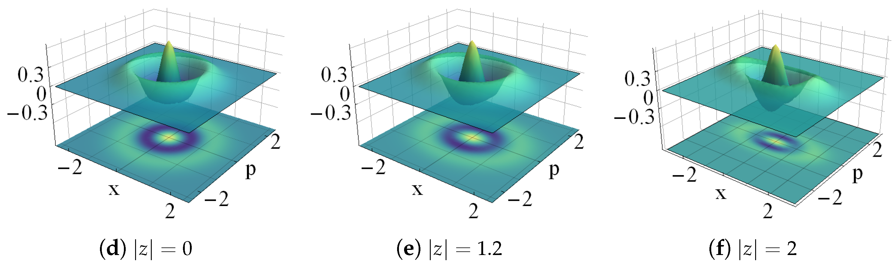
- Wigner function. In the basis of the Glauber states [2]:the Wigner function [1] of the state , with given either by (17) or (25), is expressed asIf the Wigner function is negative in at least a definite region of the phase-space, then the state is nonclassical.
References
- Wigner, E. On the Quantum Correction For Thermodynamic Equilibrium. Phys. Rev. 1932, 40, 749–759. [Google Scholar] [CrossRef]
- Glauber, R.J. Quantum Theory of Optical Coherence; Selected Papers and Lectures; Wiley: Hoboken, NJ, USA, 2007. [Google Scholar]
- Rosas-Ortiz, O. Coherent and Squeezed States: Introductory Review of Basic Notions, Properties and Generalizations. In Integrability, Supersymmetry and Coherent States; CRM Series in Mathematical Physics; Kuru, S., Negro, J., Nieto, L.M., Eds.; Springer: Berlin/Heidelberg, Germany, 2019. [Google Scholar]
- Walls, D.F. Squeezed states of light. Nature 1983, 306, 141–146. [Google Scholar] [CrossRef]
- Dodonov, V.V.; Malkin, I.A.; Man’ko, V.I. Even and odd coherent states and excitations of a singular oscillator. Physica 1974, 72, 597–615. [Google Scholar] [CrossRef]
- Stoler, D.; Salek, B.E.A.; Teich, M.C. Binomial states of the quantized radial field. Opt. Acta 1985, 32, 345–355. [Google Scholar] [CrossRef]
- Lee, C.T. Photon antibunching in a free-electron laser. Phys. Rev. A 1985, 31, 1213–1215. [Google Scholar] [CrossRef]
- Agarwal, A.S.; Tara, K. Nonclassical properties of states generated by the excitations on a coherent state. Phys. Rev. A 1991, 43, 492–497. [Google Scholar] [CrossRef]
- Aczel, A.D. Entanglement; Plume: New York, NY, USA, 2013. [Google Scholar]
- Nielsen, M.A.; Chuang, I.L. Quantum Theory and Quantum Information; Cambridge University Press: Cambridge, UK, 2000. [Google Scholar]
- Kim, M.S.; Son, W.; Buzek, V.; Knight, P.L. Entanglement by a beam splitter: Nonclassicality as a prerequisite for entanglement. Phys. Rev. A 2002, 65, 032323. [Google Scholar] [CrossRef]
- Scheel, S.; Welsch, D.G. Entanglement generation and degradation by passive optical devices. Phys. Rev. A 2001, 64, 063811. [Google Scholar] [CrossRef]
- Rosas-Ortiz, O.; Castanos, O.; Schuch, D. New supersymmetry-generated complex potentials with real spectra. J. Phys. A: Math. Theor. 2015, 48, 445302. [Google Scholar] [CrossRef]
- Blanco-Garcia, Z.; Rosas-Ortiz, O.; Zelaya, K. Interplay between Riccati, Ermakov and Schrödinger equations to produce complex-valued potentials with real energy spectrum. Math. Meth. Appl. Sci. 2019, 42, 4925–4938. [Google Scholar] [CrossRef]
- Bagarello, F.; Passante, R.; Trapani, C. (Eds.) Non-Hermitian Hamiltonians in Quantum Physics; Springer: Cham, Switzerland, 2016. [Google Scholar]
- Moiseyev, N. Non-Hermitian Quantum Mechanics; Cambridge University Press: New York, NY, USA, 2011. [Google Scholar]
- Mosk, A.P.; Lagendijk, A.; Lerosey, G.; Fink, M. Controlling waves in space and time for imaging and focusing in complex media. Nat. Photonics 2012, 6, 282–292. [Google Scholar] [CrossRef]
- Bender, C.M. Making sense of non-Hermitian Hamiltonians. Rep. Prog. Phys. 2007, 70, 947–1018. [Google Scholar] [CrossRef]
- Fernandez, H.M.; Guardiola, R.; Ros, J.; Znojil, M. Strong-coupling expansions for the PT-symmetric oscillators V(x) = a(ix) + b(ix)2 + c(ix)3. J. Phys. A: Math. Gen. 1998, 31, 10105–10112. [Google Scholar] [CrossRef]
- Fakhri, H.; Mojaveri, B.; Dehghani, A. Coherent states and Schwinger models for pseudo generalization of the Heisenberg algebra. Mod. Phys. Lett. A 2009, 24, 2039–2051. [Google Scholar] [CrossRef]
- Faisal, F.H.M. Theory of Multiphoton Processes; Springer: New York, NY, USA, 1987. [Google Scholar]
- Simon, D.S.; Jaeger, G.; Sergienko, A.V. Quantum Metrology, Imaging, and Communication; Springer: New York, NY, USA, 2017. [Google Scholar]
- Dey, S.; Fring, A.; Hussin, V. A Squeezed Review on Coherent States and Nonclassicality for Non-Hermitian Systems with Minimal Length. In Coherent States and Their Applications; Springer Proceedings in Physics; Antoine, J.P., Bagarello, F., Gazeau, J.P., Eds.; Springer: Cham, Switzerland, 2018; Volume 205. [Google Scholar]
- Rosas-Ortiz, O.; Zelaya, K. Bi-Orthogonal Approach to Non-Hermitian Hamiltonians with the Oscillator Spectrum: Generalized Coherent States for Nonlinear Algebras. Ann. Phys. 2018, 388, 26–53. [Google Scholar] [CrossRef]
- Jaimes-Nájera, A.; Rosas-Ortiz, O. Interlace properties for the real and imaginary parts of the wave functions of complex-valued potentials with real spectrum. Ann. Phys. 2017, 376, 126–149. [Google Scholar] [CrossRef]
- Zelaya, K.D.; Rosas-Ortiz, O. Optimized Binomial Quantum States of Complex Oscillators with Real Spectrum. J. Phys. Conf. Ser. 2016, 698, 012026. [Google Scholar] [CrossRef]
- Olver, F.W.J.; Lozier, D.W.; Boisvert, R.F.; Clark, C.W. (Eds.) NIST Handbook of Mathematical Functions; Cambridge University Press: Cambridge, UK, 2010. [Google Scholar]
- Abraham, P.B.; Moses, H.E. Changes in potentials due to changes in the point spectrum: Anharmonic oscillators with exact solutions. Phys. Rev. A 1980, 22, 1333–1340. [Google Scholar] [CrossRef]
- Mielnik, B. Factorization method and new potentials with the oscillator spectrum. J. Math. Phys. 1984, 25, 3387–3389. [Google Scholar] [CrossRef]
- Zelaya, K. Non-Hermitian and Time-Dependent Systems: Exact Solutions, Generating Algebras and Nonclassicality of Quantum States. Ph.D. Thesis, Cinvestav: Physics Department, Mexico City, Mexico, 2019. [Google Scholar]
- Mielnik, B.; Rosas-Ortiz, O. Factorization: Little or great algorithm? J. Phys. A Math. Gen. 2004, 37, 10007–10035. [Google Scholar] [CrossRef]
- Glauber, R.J. Coherent and incoherent states of the radiation field. Phys. Rev. 1963, 131, 2766–2788. [Google Scholar] [CrossRef]
- Sudarshan, E.C.G. Equivalence of semiclassical and quantum mechanical descriptions of statistical light beams. Phys. Rev. Lett. 1963, 10, 277–279. [Google Scholar] [CrossRef]
- Hollenhorst, J.N. Quantum limits on resonant-mass gravitational-radiation detectors. Phys. Rev. D 1979, 19, 1669–1679. [Google Scholar] [CrossRef]
- Caves, C.M. Quantum-mechanical noise in an interferometer. Phys. Rev. D 1981, 23, 1693–1708. [Google Scholar] [CrossRef]
- Dodonov, V.V.; Man’ko, V.I. (Eds.) Theory of Nonclassical States of Light; Taylor and Francis: New York, NY, USA, 2003. [Google Scholar]
- Dey, S.; Hussin, V. Entangled squeezed states in noncommutative spaces with minimal length uncertainty relations. Phys. Rev. D 2015, 91, 124017. [Google Scholar] [CrossRef]
- Dey, S. Q-deformed noncommutative cat states and their nonclassical properties. Phys. Rev. D 2015, 91, 044024. [Google Scholar] [CrossRef]
- Dey, S.; Fring, A.; Hussin, V. Nonclassicality versus entanglement in a noncommutative space. Int. J. Mod. Phys. B 2017, 31, 1650248. [Google Scholar] [CrossRef]
- Zelaya, K.; Rosas-Ortiz, O.; Blanco-Garcia, Z.; Cruz, S. Completeness and Nonclassicality of Coherent States for Generalized Oscillator Algebras. Adv. Math. Phys. 2017, 2017, 7168592. [Google Scholar] [CrossRef]
- Mojaveri, B.; Dehghani, A.; Bahrbeig, R.J. Excitation on the para-Bose states: Nonclassical properties. Eur. Phys. J. Plus 2018, 133, 346. [Google Scholar] [CrossRef]
- Mojaveri, B.; Dehghani, A.; Bahrbeig, R.J. Nonlinear coherent states of the para-Bose oscillator and their non-classical features. Eur. Phys. J. Plus 2018, 133, 529. [Google Scholar] [CrossRef]
- Fernandez, D.J.; Hussin, V.; Rosas-Ortiz, O. Coherent states for Hamiltonians generated by supersymmetry. J. Phys A: Math. Theor. 2007, 40, 6491–6511. [Google Scholar] [CrossRef]
- Man’ko, V.I.; Marmo, G.; Sudarshan, E.C.G.; Zaccaria, F. F-oscillators and nonlinear coherent states. Phys. Scr. 1997, 55, 528–541. [Google Scholar] [CrossRef]
- Fernandez, C.D.J.; Nieto, L.M.; Rosas-Ortiz, O. Distorted Heisenberg Algebra and Coherent States for Isospectral Oscillator Hamiltonians. J. Phys. A Math. Gen. 1995, 28, 2693–2708. [Google Scholar] [CrossRef]
- Rosas-Ortiz, J.O. Fock-Bargman Representation of the Distorted Heisenberg Algebra. J. Phys. A Math. Gen. 1996, 29, 3281–3288. [Google Scholar] [CrossRef]
- Mandel, L. Sub-Poissonian photon statistics in resonance fluorescence. Opt. Lett. 1979, 4, 205–207. [Google Scholar] [CrossRef]


© 2019 by the authors. Licensee MDPI, Basel, Switzerland. This article is an open access article distributed under the terms and conditions of the Creative Commons Attribution (CC BY) license (http://creativecommons.org/licenses/by/4.0/).
Share and Cite
Zelaya, K.; Dey, S.; Hussin, V.; Rosas-Ortiz, O. Nonclassical States for Non-Hermitian Hamiltonians with the Oscillator Spectrum. Quantum Rep. 2020, 2, 12-38. https://doi.org/10.3390/quantum2010002
Zelaya K, Dey S, Hussin V, Rosas-Ortiz O. Nonclassical States for Non-Hermitian Hamiltonians with the Oscillator Spectrum. Quantum Reports. 2020; 2(1):12-38. https://doi.org/10.3390/quantum2010002
Chicago/Turabian StyleZelaya, Kevin, Sanjib Dey, Veronique Hussin, and Oscar Rosas-Ortiz. 2020. "Nonclassical States for Non-Hermitian Hamiltonians with the Oscillator Spectrum" Quantum Reports 2, no. 1: 12-38. https://doi.org/10.3390/quantum2010002
APA StyleZelaya, K., Dey, S., Hussin, V., & Rosas-Ortiz, O. (2020). Nonclassical States for Non-Hermitian Hamiltonians with the Oscillator Spectrum. Quantum Reports, 2(1), 12-38. https://doi.org/10.3390/quantum2010002