Detection of Traffic Lights and Status (Red, Yellow and Green) in Images with Different Environmental Conditions Using Architectures from Yolov8 to Yolov12

Abstract

Given that approximately 70% of traffic accidents are attributable to driver-related factors, it is necessary for vehicles to incorporate technologies that reduce risk through preventive actions derived from traffic-scene analysis. Interpreting the driving environment is non-trivial and is commonly decomposed into sub-tasks; among them, traffic light perception is critical due to its role in regulating vehicular flow. This paper evaluates five YOLO CNN families (YOLOv8–YOLOv12) on two tasks: (i) traffic light detection and (ii) traffic light state recognition (green, yellow, red). The evaluation uses a hybrid dataset comprising the public LISA traffic light dataset and a custom dataset with images from Mexico City captured under diverse lighting conditions—a relevant setting given the city’s high traffic intensity. The results show mAP@0.50 = 94.4–96.3% for traffic light detection and mAP@0.50 = 99.3–99.4% for traffic light state recognition, indicating that modern YOLO variants provide highly reliable performance for both tasks under natural illumination variability.

1. Introduction

According to the 2025 TomTom Traffic Index report [1], Mexico City ranks as the most congested urban area worldwide, a condition that contributes to several mobility-related issues, including an increased incidence of traffic accidents. Findings from studies conducted by the Mexican Ministry of Communications and Transportation (SCT) indicate that approximately 71% of traffic incidents are attributable to driver-related factors. Of this percentage, 20% result from recklessness or inattention, 12% from speeding, 11% from lane violations, and another 11% from failing to maintain a safe following distance [2]. Additionally, emerging technologies, particularly mobile phones, have rapidly become a major source of driver distraction [3]. In response, various intelligent vehicular technologies have been developed to support preventive actions and reduce accident rates [4].

Recent advances in intelligent transportation systems have significantly impacted road safety, mobility, and the development of autonomous vehicles (AVs) [5], one of the aspects that has benefited greatly is automated driving systems (ADSs) [6], which are expected to improve road accident rates attributed to drivers by 94% [7,8]. Consequently, intelligent decision-making modules embedded within AVs aim to minimize these human-factor failures by generating safe and consistent driving actions [9,10].

Within the broader framework of advanced driver assistance systems (ADASs), several perception and decision-making challenges must be solved to achieve Levels 3–5 autonomy, as defined in the SAE taxonomy. These challenges include vehicle detection and tracking [11], traffic sign and traffic light recognition [12,13,14], pedestrian detection [15,16], lane and curve detection [17], road object localization [18,19,20], and traffic scene analysis [21], among others [22]. Addressing these tasks requires the integration of specialized hardware capable of processing multimodal sensor data (camera, LiDAR, radar), as well as software based on artificial intelligence (AI) capable of interpreting such information and generating optimal driving decisions [23].

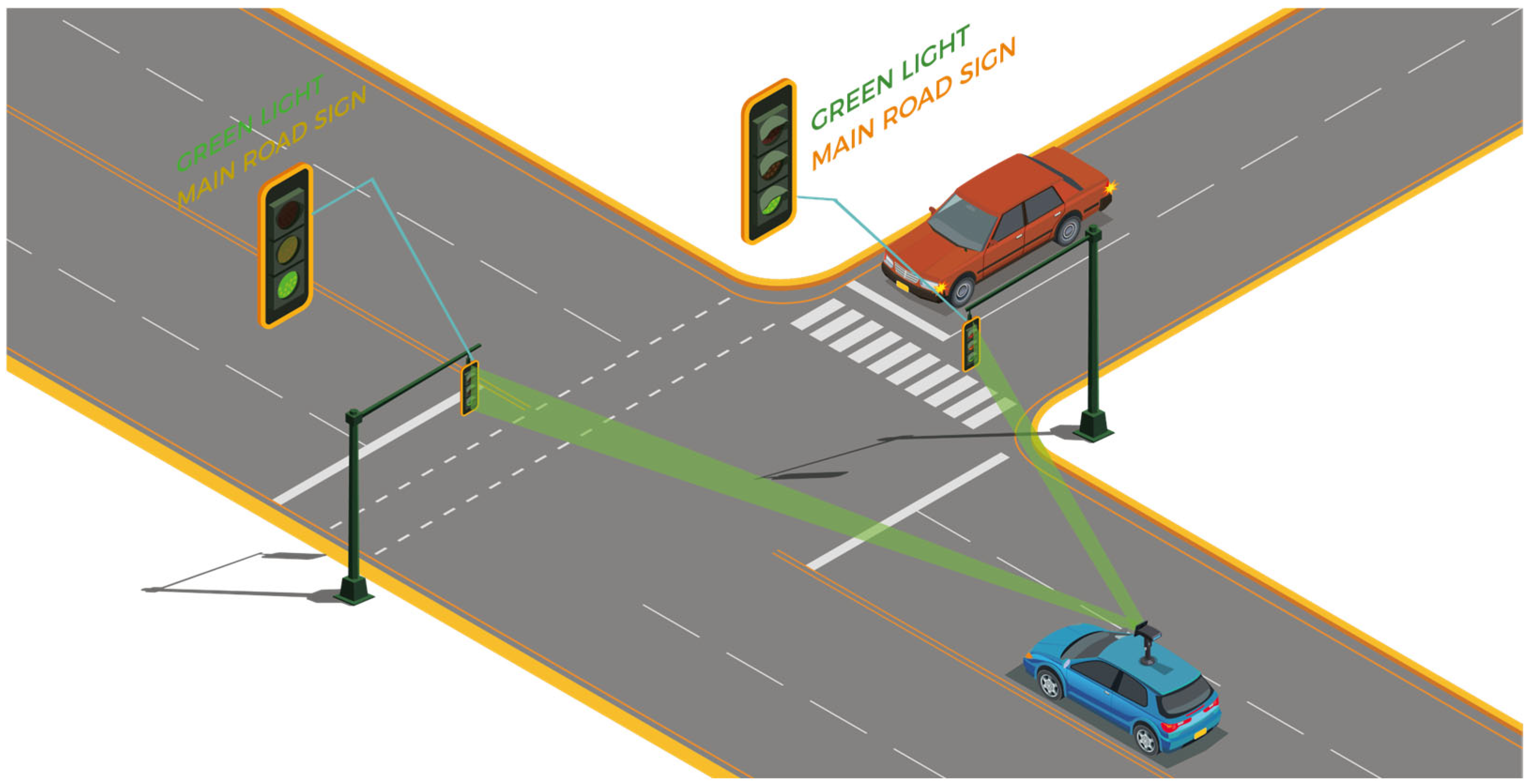
Traffic lights represent a fundamental component for regulating vehicle flow at intersections; therefore, an autonomous vehicle must be capable of detecting them and correctly identifying their state (green, yellow, or red) to comply with traffic regulations and operate safely within the road network [14]. Figure 1 illustrates an example of an AV equipped with an ADS module for traffic light detection and state recognition.

1.1. Introduction Background and Scope of This Study

Traffic lights are a core element within the broader problem of perceiving and interpreting the navigation environment for autonomous vehicles equipped with automated driving systems (ADSs) and advanced driver assistance systems (ADASs). As regulatory devices, traffic lights regulate vehicular flow at intersections and crossings; consequently, their detection and state recognition constitute a recognized research challenge in autonomous driving [24]. Improving reliability in traffic light perception is essential to enhancing road safety and optimizing traffic flow. Despite remarkable progress, several open challenges remain. A clear understanding of the relevance of traffic light perception and the associated failure modes is therefore crucial to developing more effective solutions.

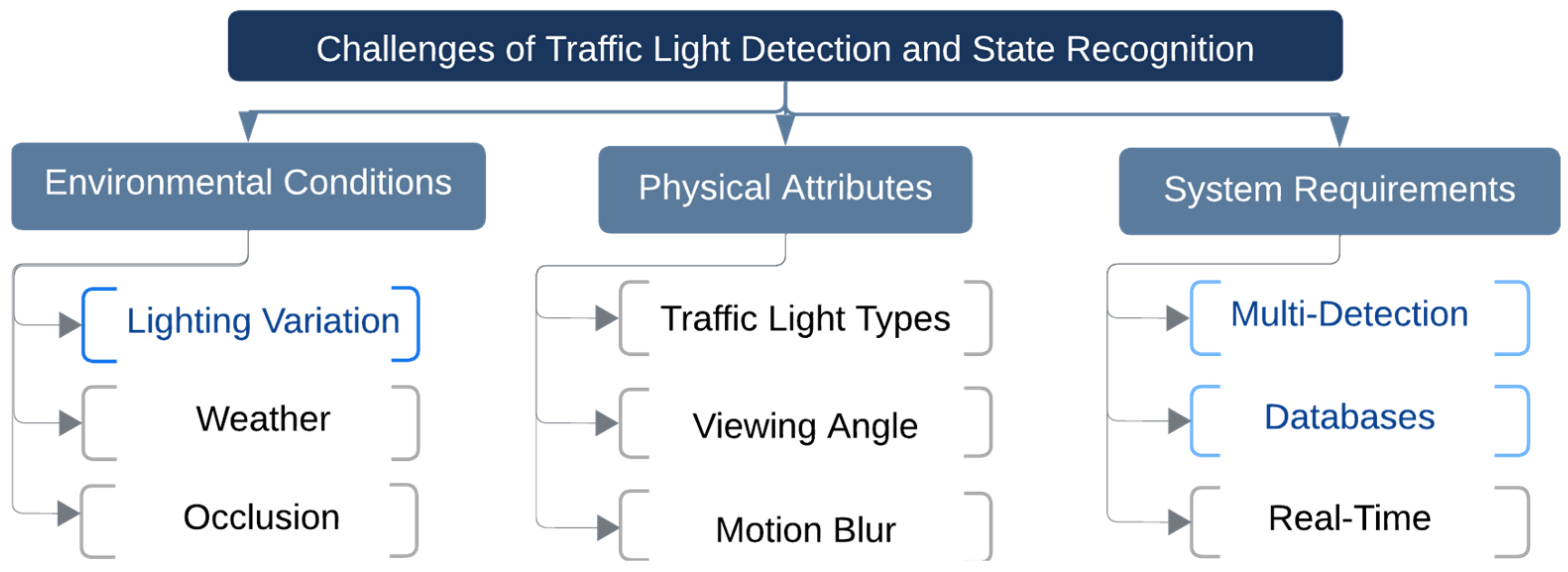
Automatic traffic light interpretation must operate in uncontrolled outdoor environments, where performance depends on environmental variability (e.g., illumination, weather, occlusions) and system-level response requirements (latency, throughput, memory). These challenges can be organized into three overarching categories—environmental conditions, physical attributes, and system requirements—within which learning-based algorithms typically provide task-specific responses depending on the primary difficulty being addressed.

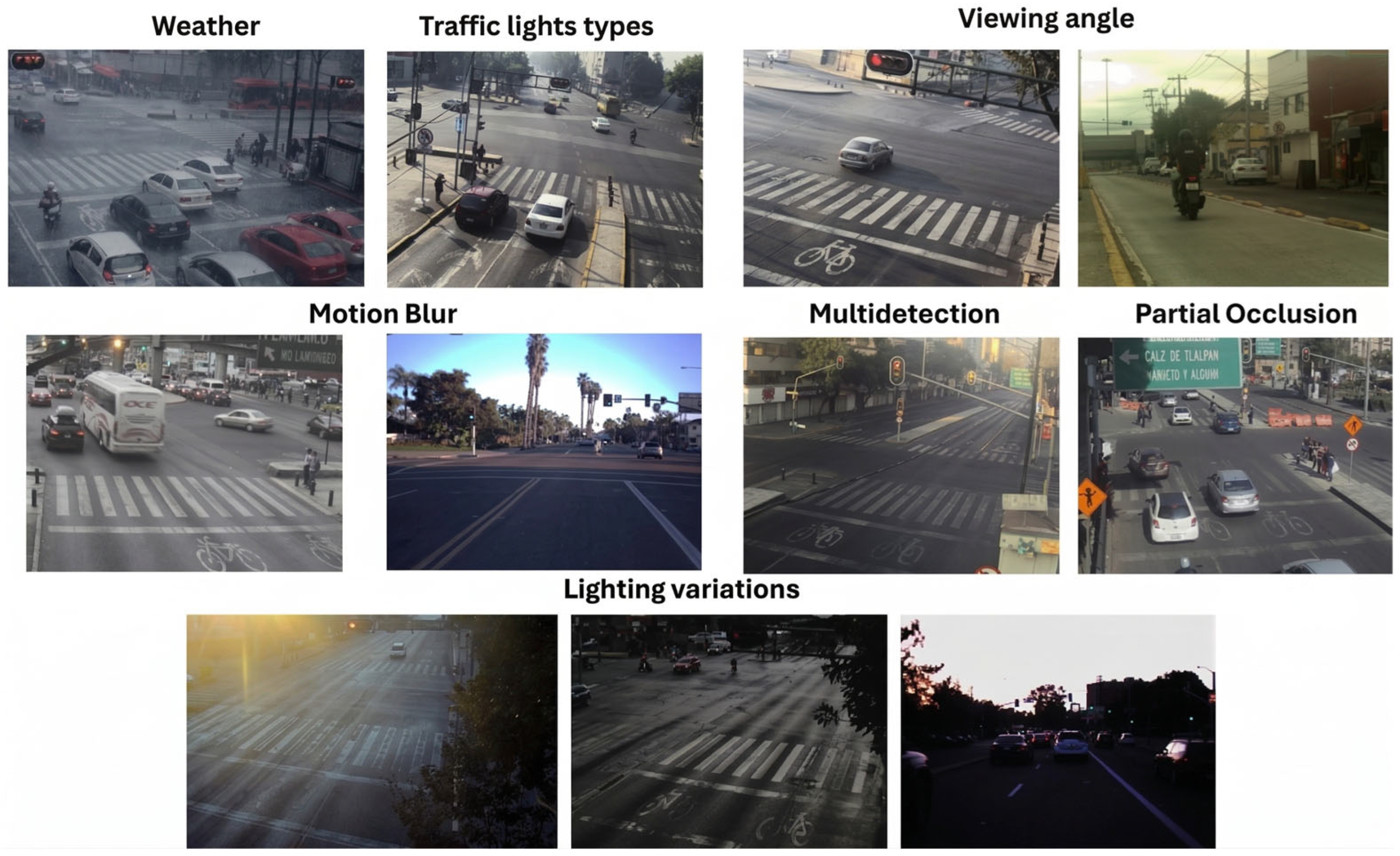
Figure 2 illustrates the challenges involved in traffic light detection and state recognition, grouped into environmental conditions, physical attributes, and system requirements. Figure 3 presents example images illustrating representative challenges faced by automatic traffic light detection.

Within this context, the present study focuses on the challenge of natural illumination variability, which falls under environmental conditions. Because traffic lights are installed outdoors, they are exposed to changes in illumination caused by sunlight and indirect lighting effects. Addressing this problem is non-trivial; automatic detection and state-interpretation systems can be adversely affected by shadows, specular reflections that alter apparent color, insufficient illumination, and over-exposure, among other factors.

A second challenge tackled in this work is simultaneous multi-instance detection a system-level requirement for practical deployment since intersections commonly contain “multiple traffic lights”. This is compounded by the heterogeneity of signal types (vehicular, pedestrian, and bicycle signals) that may coexist and interact within the same scene; accordingly, the algorithm is trained to detect all vehicular traffic lights present in the field of view.

Finally, we address the challenge of dataset design and domain specificity, which has a significant impact on real-world deployment (e.g., in Mexico City). Cities exhibit distinctive traffic-scene characteristics such as extreme congestion and complex intersection layouts that induce domain shifts the CNN must learn to model and generalize over. Consequently, dataset composition and curation become critical to ensure robust performance beyond controlled benchmarks.

1.2. State of the Art

Research in computer vision and artificial intelligence has produced a broad family of Convolutional Neural Network (CNN)-based detectors that underpin robust perception technologies across domains; a key application is ADAS/ADS perception for identifying and recognizing elements in the driving environment [18]. Humans acquire driving cues visually; building on this premise, current perception pipelines aim to replicate these capabilities artificially [25]. Within road-scene understanding, traffic signals constitute a critical source of regulatory information. For example, Galvão et al. [16] summarize perception systems for traffic light and vehicle detection, reporting a strong shift toward deep learning for object detection in driving environments. Prominent detector families include YOLO (You Only Look Once), SSD (Single-Shot MultiBox Detector), Faster R-CNN, and Mask R-CNN; common challenges remain adverse weather, illumination changes, and occlusion. Liang et al. [26] examine object detectors for autonomous vehicles (AVs) and highlight sensor fusion processed through CNN-based architectures (e.g., YOLO, Faster R-CNN) as an effective strategy, while emphasizing persistent issues such as real-time performance, robustness under adverse conditions, the accuracy–efficiency trade-off, and multimodal learning. Regarding datasets, Karangwa et al. [27] compile corpora widely used for vehicle detection, and Liu et al. [28] analyze 265 autonomous-driving datasets from the perspectives of sensing modality, data volume, tasks, and contextual conditions. Complementarily, Song et al. [29] evaluate synthetic datasets, discussing their benefits and drawbacks for training intelligent models. In traffic-sign analysis, Zhao et al. [30] propose TSD-YOLO, a hybrid model for four signal categories (Warning, Information, Regulatory, Complementary) leveraging Mamba and YOLO, trained on MTSD, TT100K, and GTSDB; they report mean accuracies of 86.44%, 70.95%, 82.72%, and 76.59% for each class, respectively. Finally, beyond detection, recognition and interpretation of traffic signals [31], information remain essential for enforcing driving rules, where CNN-based approaches are widely adopted [28]. Pavlitska et al. [32] survey the main traffic light detection datasets and compare representative methods, noting the prevalence of YOLO, Faster R-CNN, and ResNeSt backbones.

Yang et al. [33] detect traffic lights using an improved YOLOv4-based detector trained on the LISA dataset, reporting 90% accuracy with 15 ms inference time. In comparisons against Faster R-CNN and SSD, YOLOv4 achieves a more favorable speed–accuracy trade-off. Yoneda et al. [34] develop a method to identify sun-glare regions using CNN-based visual explanations: the network produces Grad-CAM attention maps, and the general direction of glare is then estimated via time-series analysis. This approach supports robust image recognition by explicitly modeling how direct and building-reflected sunlight degrades visibility.

Wang et al. [35] propose detecting traffic lights using an improved YOLOv4 trained on the LISA database, achieving 90% accuracy with inference times of 15 ms. They compare YOLOv4 with Faster R-CNN and SSD, finding the former to perform better and show a better balance of speed and accuracy. Song et al. [36] introduce Mosaic-9 to augment the training set and enhance generalization to real-world scenarios; they curate 2000 images containing traffic lights in diverse positions and states (red, green, yellow) and integrate a Squeeze-and-Excitation (SE) attention mechanism, achieving 99.5% accuracy at 74 FPS. Meanwhile, Kumar et al. [21] present 3D YOLO-SM (3D Depth Perception based on 2D Object Detection with YOLO, with an integrated Neural State Machine (NSM)), which combines an enhanced YOLOv8-based detector with an NSM and uses images from a stereo camera. Their model attains mAP@0.5 scores of 92.5% on LISA and 89.3% on Bosch.

Table 1. Summary of the most relevant studies focused on the detection and state recognition of traffic lights: a comparative analysis of datasets, methods, and model performance.

Author	Dataset	Problem	Image	Model	Accuracy	Observations
Ma et. al. 2026 [40]	Owned with images from Indonesia and China	Traffic light status recognition	1000	YOLO v12n	0.73 during real-time operation	Includes day and night conditions, and various weather conditions (clear and rainy)
Munir and Lin 2025 [41]	Public TN-TLD Dataset (Taiwan Nighttime Traffic Light)	Traffic light status recognition	36,050	LNT-YOLO	mAP@0.5 = 0.781	Traffic light detection during night driving
Tammisetti et. 2025 [42]	Mixed public datasets: Kitty, Kaggle, Carla, LISA, Cityscapes and Eurocity	Traffic light status recognition	335	YOLOv8, Meta-YOLOv8	0.93	Meta-YOLOv8 is used to improve YOLOv8 performance
Yagob and Sasiadek 2025 [43]	Github dataset 2023 GitHub y de Roboflow	Traffic light status recognition	650	YOLOv8	Traffic light 0.943 Red 0.992 Yellow 0.995 Green 0.853	Depthwise Separable Convolutions (DISCs) are integrated throughout the backbone and head
Khaled et. al. 2025 [44]	Own, real Mississippi data and simulated data using RoadRunner	Traffic light recognition and classification of flashing traffic lights	54,000	YOLOv10n ResNet-18 LSTM	Red (1.00), Yellow (1.00), Green (0.98), Flashing Red (0.92) and Flashing Yellow (0.92)	NVIDIA A100 GPUs were used, achieving a performance of 67.15 FPS
Proposed 2026	Mixed database: Own database of images of Mexico City and public LISA database	Traffic light recognition and status classification	Frames of complete scenarios 22,217 and 36,000 traffic light segments	Yolov8, Yolov9 Yolov10, Yolov11, Yolov12	Traffic light 0.93 Red 1.0 Yellow 1.0 Green 0.98	Performance comparison of YOLO v8 to YOLO v12 in real-time images under different natural lighting conditions

presents a concise summary of recent studies addressing traffic light detection and state recognition (green, yellow, red). Most works adopt YOLO-based CNNs in different versions; the last row reports the approach proposed in this study. The contribution of our work focuses on detecting and interpreting traffic light information with YOLO [37,38,39], one of the most frequently cited detector families for this task. A key challenge is illumination variability, since performance is highly sensitive to diurnal changes in light level. To mitigate this, we train with a hybrid dataset that combines the public LISA dataset with a proprietary dataset captured at 10 locations in Mexico City across different times of day. Our goal is to identify the YOLO version and hyperparameter regime that best address detection and state recognition under varying illumination. Accordingly, we evaluate the five latest YOLO versions—YOLOv8m, YOLOv9m, YOLOv10m, YOLOv11m, and YOLOv12m—and determine which offers the best accuracy–inference-speed trade-off.

Section 1 reviews related studies and methodologies. Section 2 describes the proposed system and methodology and outlines the theoretical foundations of the models and techniques employed. Section 3 details the experimental setup used to demonstrate the competitiveness of the proposed approach and reports the results. Section 4 presents conclusions and a discussion.

2. Materials and Methods

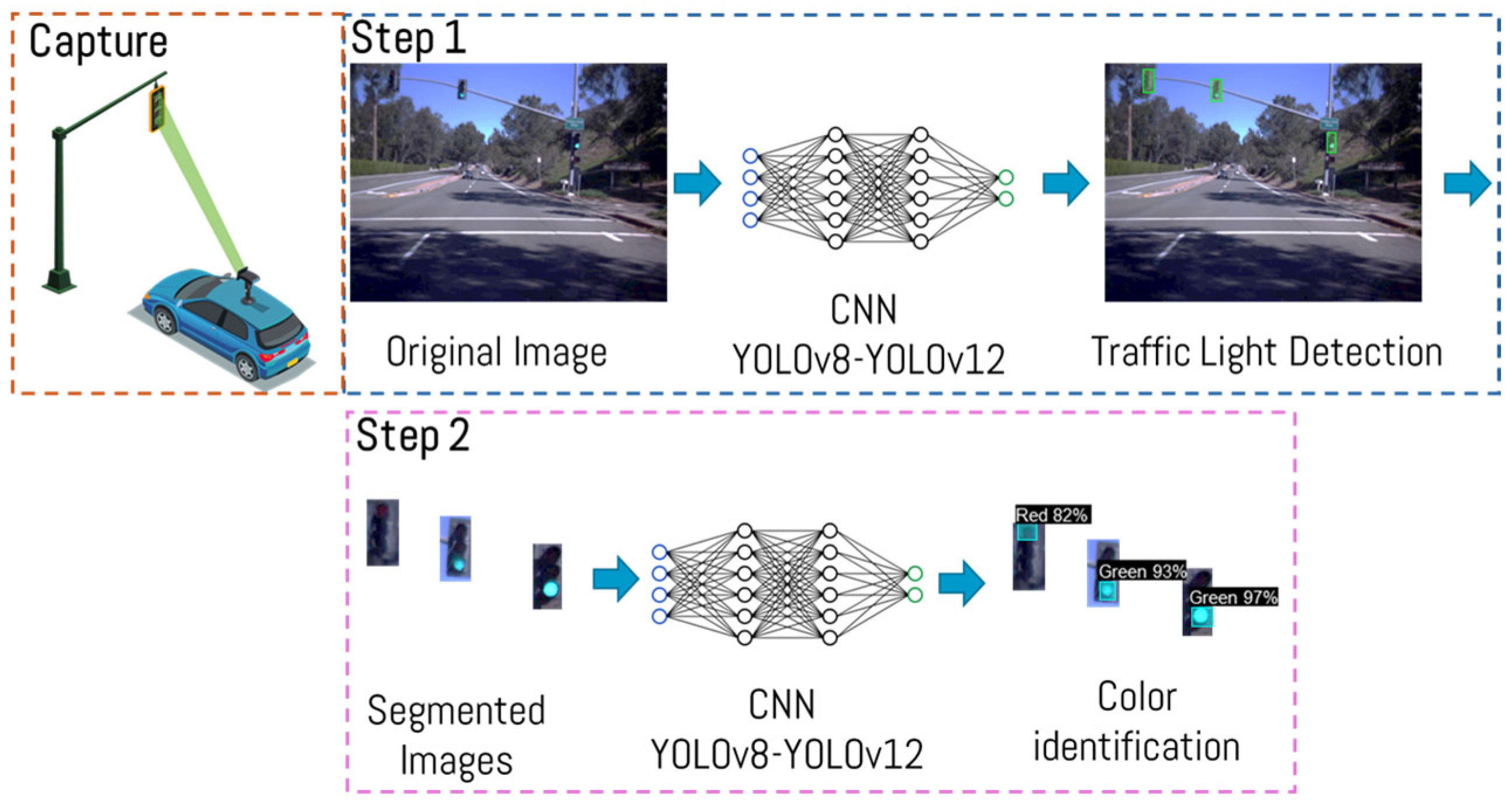
We propose a two-step methodology for traffic light perception in images. Step 1 (detection): identify all traffic lights present in the scene using YOLO-based CNNs, specifically YOLOv8m, YOLOv9m, YOLOv10m, YOLOv11m, and YOLOv12m, and report their detection performance. Step 2 (state recognition): determine the state (green, yellow, red) of each traffic light detected in Step 1. The same YOLO versions are evaluated for this second task, and their results are likewise reported.

Figure 4 depicts the end-to-end pipeline. The input image is first processed by one of the YOLO models (versions v8–v12) to perform simultaneous multi-instance detection of traffic lights. Predictions meeting a confidence threshold of 0.90 are retained, and the corresponding regions are cropped. Each crop is then passed again through the YOLO v8–v12 variants to perform the state recognition task.

2.1. Methodology

The problem is decomposed into two tasks because preliminary experiments (beyond the scope of this paper) attempting single-network joint detection and state classification by labeling each state as a separate class produced suboptimal results, particularly under natural illumination variability. Additionally, intersections in Mexico City contain numerous non-signal objects that resemble traffic lights; under low-light conditions, this visual ambiguity is exacerbated. Consequently, we adopt a two-stage strategy: (i) traffic light detection, followed by (ii) state recognition (green, yellow, red).

A primary objective is to ensure balanced generalization under varying natural lighting (i.e., across different times of day). Moreover, since the algorithm will be assessed in Mexico City, a highly congested urban setting with many distractors, we construct a hybrid dataset combining (i) the LISA public dataset and (ii) a custom dataset captured at 10 intersection locations across the city and at multiple times of day (see Section 2.2). This enables a controlled study to identify the YOLO version and hyperparameter configuration that best address detection and state recognition under illumination shifts.

We select the latest YOLO families (v8–v12, “m” variants) due to their high real-time accuracy, single-stage design that naturally supports joint localization and classification, and robustness to variations in illumination, weather, and distance. YOLO also performs well on small objects such as traffic lights; it is straightforward to fine-tune for task-specific classes and can be deployed on low-cost embedded systems, making it an efficient, accurate, and practical solution for intelligent mobility and autonomous driving applications.

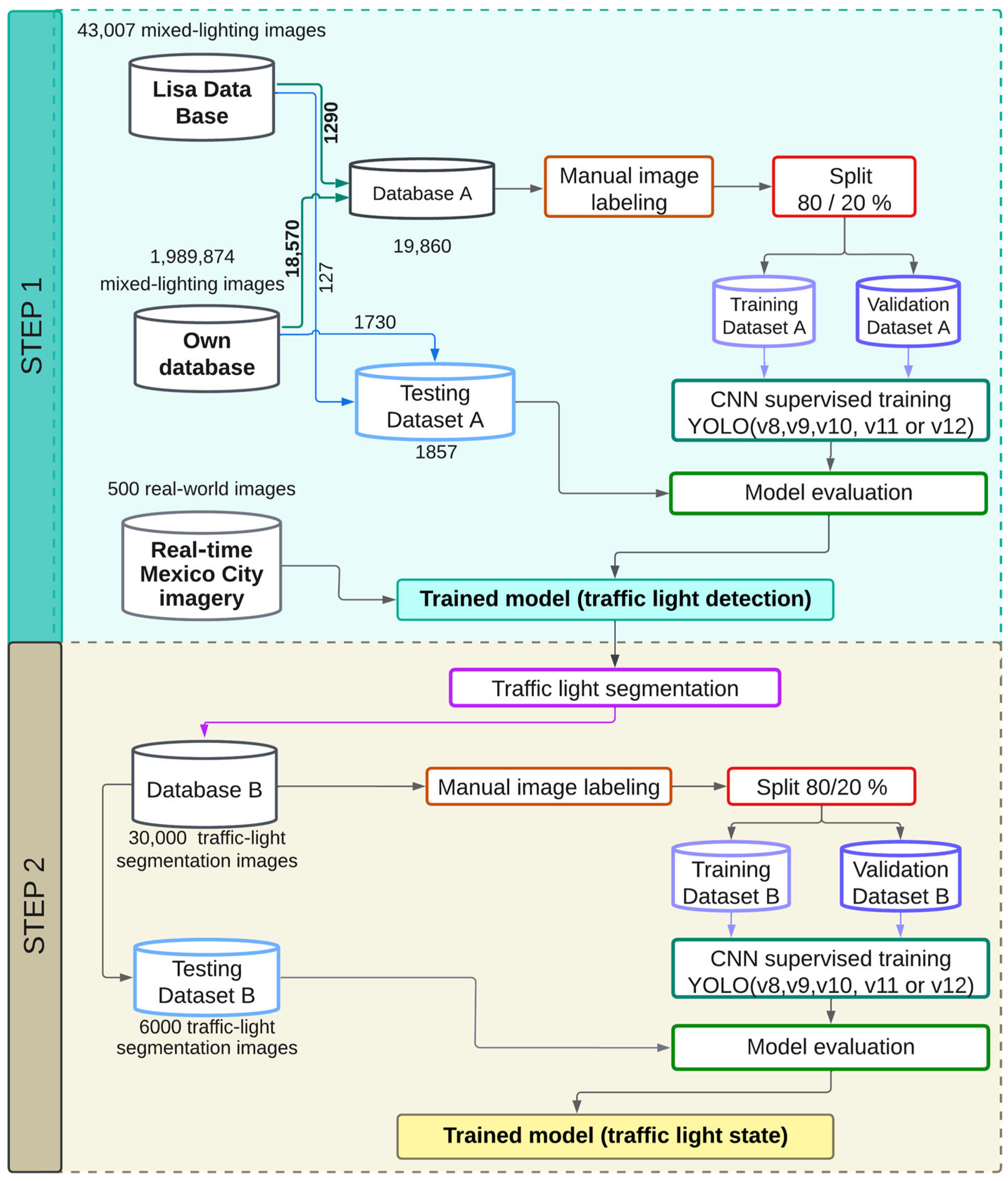
Step 1 (Traffic Light Detection). As shown in Figure 5, the first stage detects all traffic lights in road-intersection scenes. We selected 1290 images from the LISA dataset [40,41] and 18,570 images from an in-house dataset and merged them into Dataset A (19,860 images) with a single label, traffic_light. We applied an 80/20 holdout split to create Training Set A (80%) and Validation Set A (20%). Additionally, we built an independent real-time test set with 500 images captured at 10 intersections in Mexico City; this set was never used during training or validation and serves to assess model performance under real operating conditions.

Step 2 (State Recognition). After training the five YOLO variants for simultaneous multi-instance detection, we proceeded to state recognition (red/yellow/green). We generated a new image set by cropping the regions where traffic lights were detected in Step 1 (noting that multiple traffic lights may appear per scene). These crops compose Dataset B (30,000 images) annotated with three labels: trafficlight_green, trafficlight_red, and trafficlight_yellow. We applied an 80/20 holdout to obtain Training Set B (80%) and Validation Set B (20%), and we created Testing Set B with 6000 images to evaluate the state recognition models under real-world conditions.

2.2. Dataset

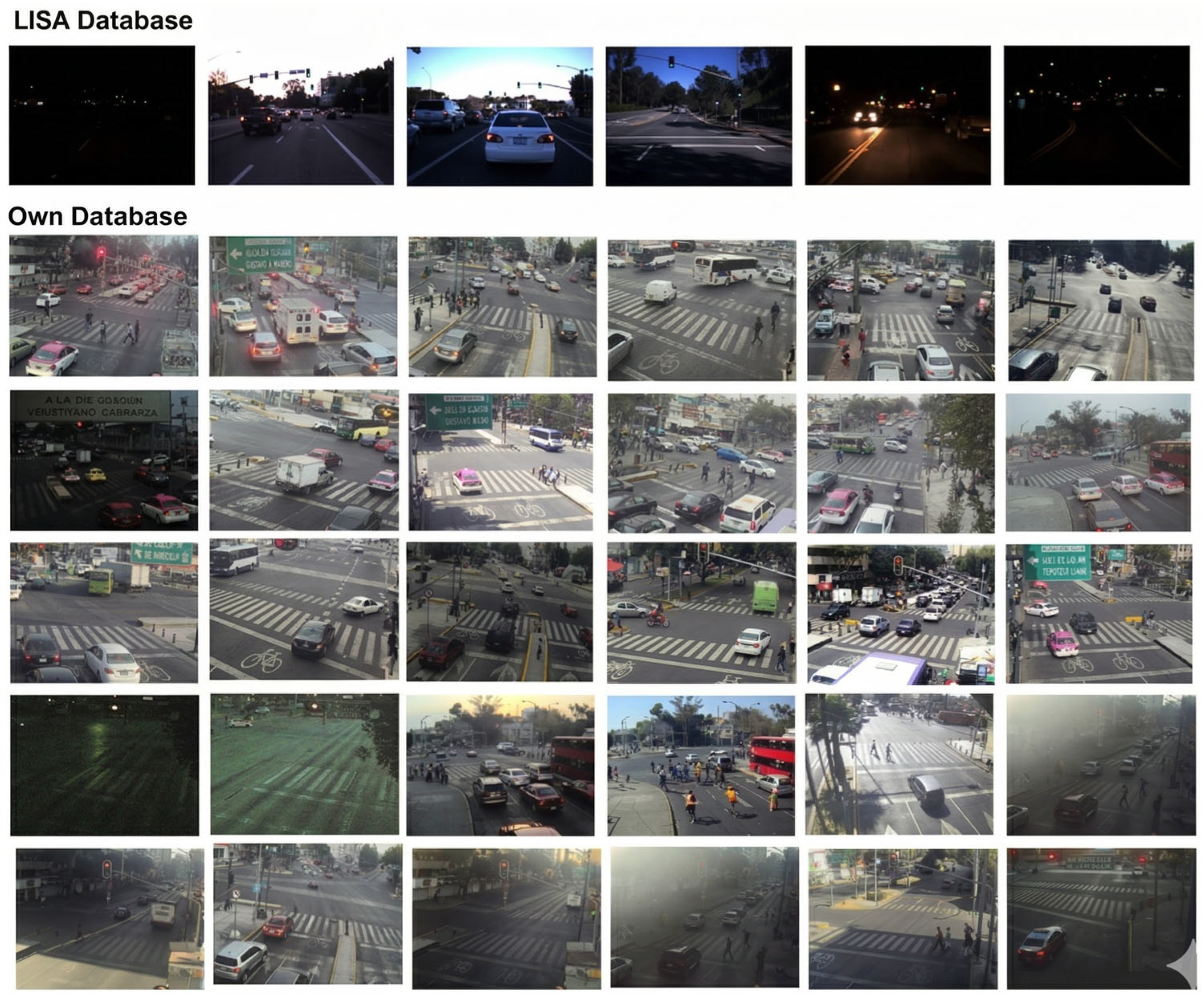
For this study, we used two data sources (see

Table 2. Datasets used for traffic light detection and state recognition.

Database	Set	Characteristics
		# Images	# Class	Class	Resolution
LISA	Traffic light detection training	1290	1	traffic_light	1280 × 960
Own		18,570			4000 × 2992
LISA	Traffic light detection testing	127	1	traffic_light	1280 × 960
Own		1730			4000 × 2992
Own and LISA mix	State recognition training	30,000	3	trafficlight_green trafficlight_yellow trafficlight_red	1280 × 960 4000 × 2992
Own and LISA mix	State recognition test	6000	3	trafficlight_green trafficlight_yellow trafficlight_red	1280 × 960 4000 × 2992
Own	Real-time traffic light detection test	500	1	traffic_light trafficlight_green trafficlight_yellow trafficlight_red	4000 × 2992

). The first is the public LISA Traffic Light Dataset [40,41], which provides sequences captured in San Diego, California (USA), under daytime and nighttime conditions at 1280 × 960 px. From LISA, we selected 1290 images for training and 127 for testing.

The second source is a proprietary dataset comprising 1,989,874 images collected at 10 intersection locations in Mexico City across different times of day, yielding variations in illumination (diurnal changes and reflectance) and environmental conditions. From this dataset, 18,570 images were selected for training and 1730 for testing. Additionally, 500 real-time images were captured from the same locations/cameras to test the trained models under operational conditions, both for traffic light detection and state recognition.

Figure 6 illustrates representative samples employed in our experiments across the training, validation, and test splits for all evaluated YOLO versions.

2.3. You Only Look Once (YOLO) Architecture

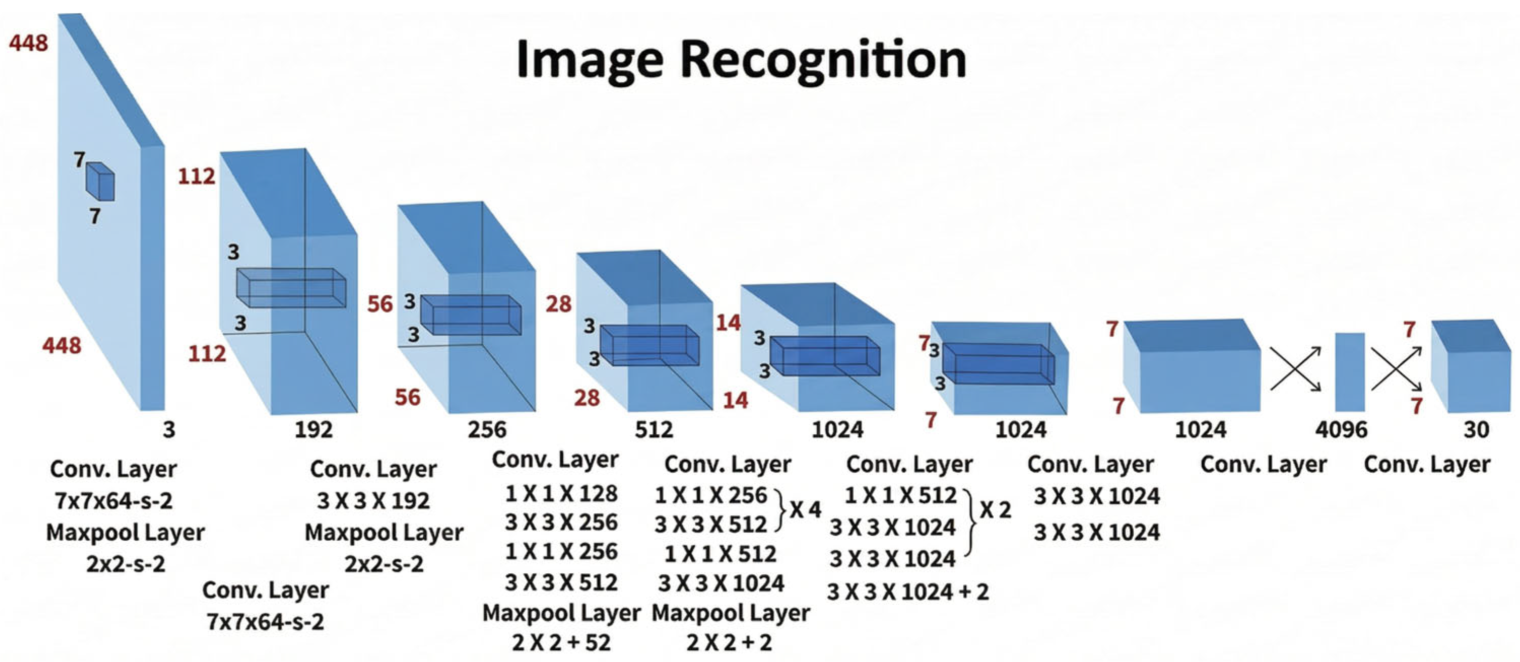
Because one objective of this study is to analyze the performance of five YOLO versions on vehicular traffic light detection and state recognition, we first provide a concise overview of the YOLO family considered in our experiments. The original YOLOv1 architecture was inspired by GoogLeNet [45]. It comprises 24 convolutional layers followed by 2 fully connected layers, producing a 7 × 7 × 30 prediction tensor for grid-based detection. Instead of the early Inception modules used in GoogLeNet, YOLOv1 employs 1 × 1 reduction layers followed by 3 × 3 convolutions, in line with the design principles popularized by Lin et al. [46].

As detailed in Figure 7, input images are resized to 448 × 448 px (RGB) before inference. Subsequent layers specify the kernel sizes, number of filters, and strides for each convolutional block; certain blocks repeat (×2, ×4). The output layer encodes the model’s prediction bounding boxes and class probabilities for each grid cell.

2.3.1. YOLOv8

The YOLOv8 model [47] supports complex tasks such as instance segmentation, keypoint/pose estimation, and oriented object detection. Key features include real-time performance, high inference speed, comprehensive Ultralytics Python tooling for training and deployment, and multiple model variants (n, s, m, l, x).

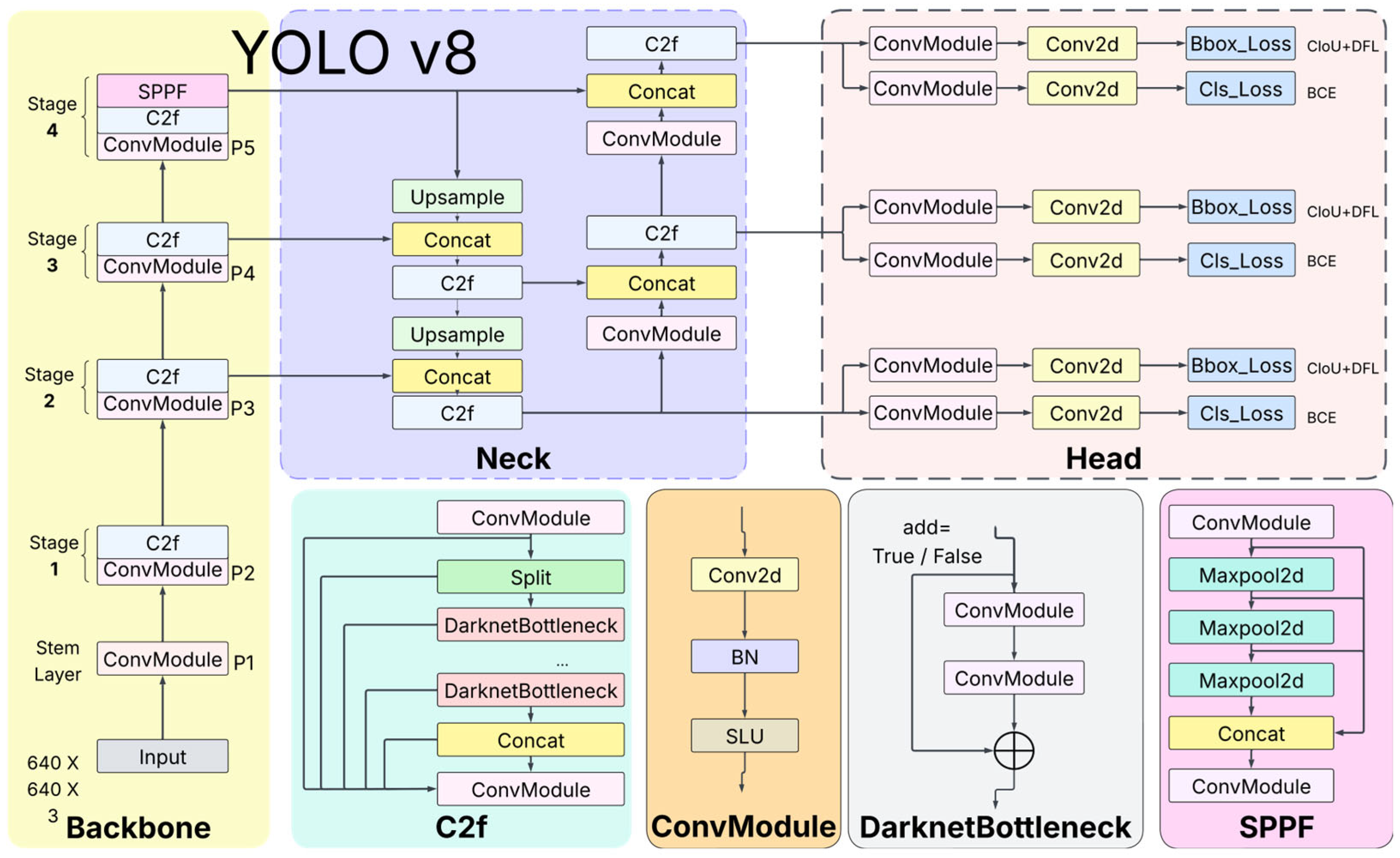
Training is simplified through an anchor-free head. However, several limitations are anticipated, including reduced sensitivity to very small objects, a higher computational cost than some earlier versions, and an increased dependence on training-data quality. As shown in Figure 8, the YOLOv8 architecture comprises three main blocks: the Backbone (feature extraction), the Neck (multi-scale feature aggregation), and the Head (prediction of classes and boxes).

2.3.2. YOLOv9

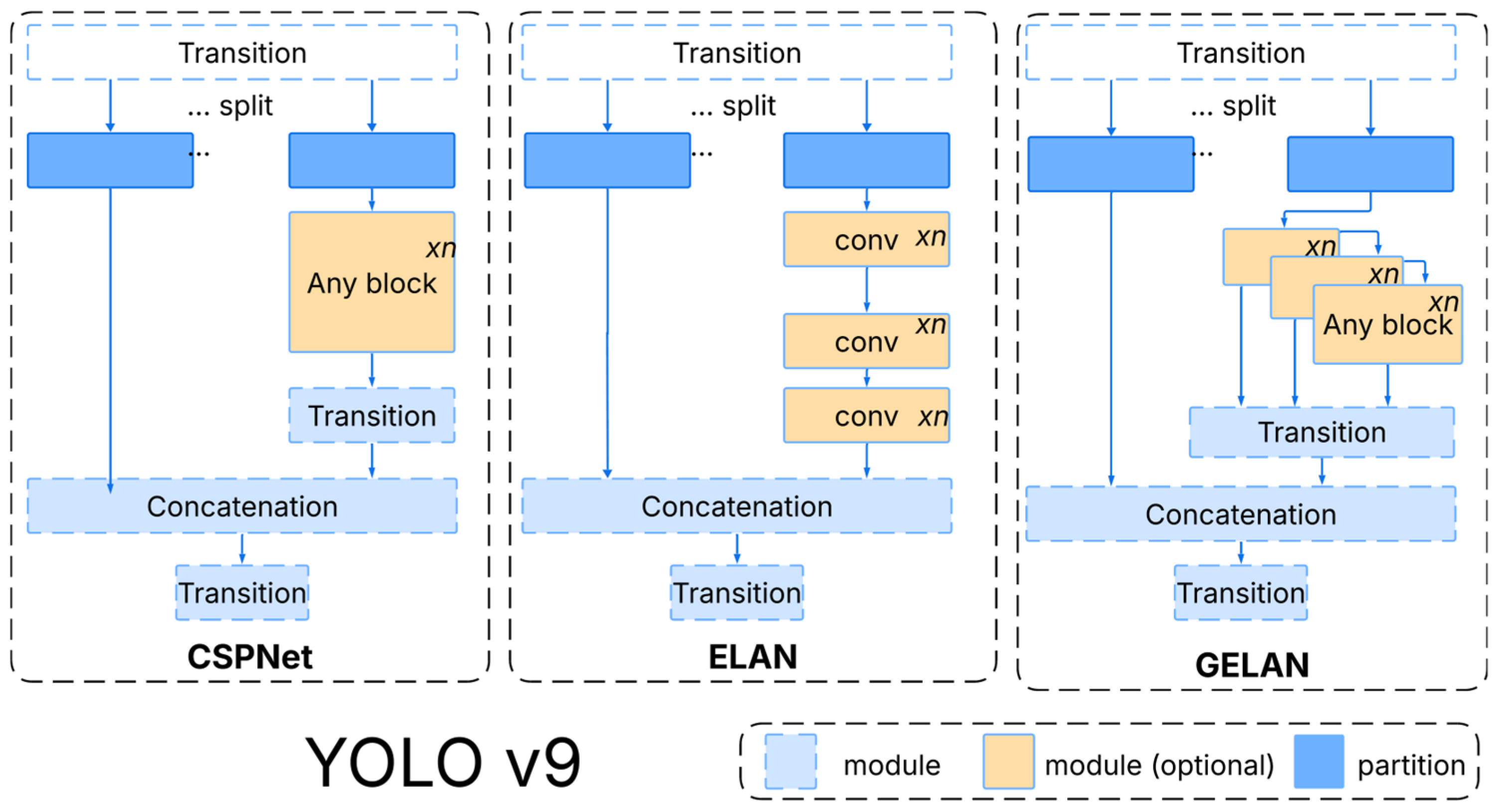
YOLOv9 [48,49] explicitly addresses information loss as network depth increases. To this end, it introduces Programmable Gradient Information (PGI), a supervisory framework to preserve gradient quality, and a hybrid architecture, the Generalized Efficient Layer Aggregation Network (GELAN), which combines the strengths of CSPNet and ELAN to improve efficiency, accuracy, and adaptability while remaining conceptually aligned with prior YOLO designs.

As shown in Figure 9, there are three significant differences compared to previous versions. The first is the incorporation of reversible functions that address the information bottleneck problem. Their use guarantees reduced information loss by reconstructing the original input from the network outputs. The second change is the integration of Programmable Gradient Information (PGI). Implementing reversible functions necessitates a training method that ensures accurate gradient descent for both deeper and surface layers. PGI optimizes inference in the main branch, while mitigating information loss from deeper layers in the reversible auxiliary branch. Additionally, it ensures monitoring for information loss in multilevel information, enabling the detection of objects of varying sizes. Finally, YOLOv9 incorporates the Generalized Efficient Layer Aggregation Network (GE-LAN), which aims to achieve a connection adapted to GPIs, allowing for the integration of the various blocks.

2.3.3. YOLOv10

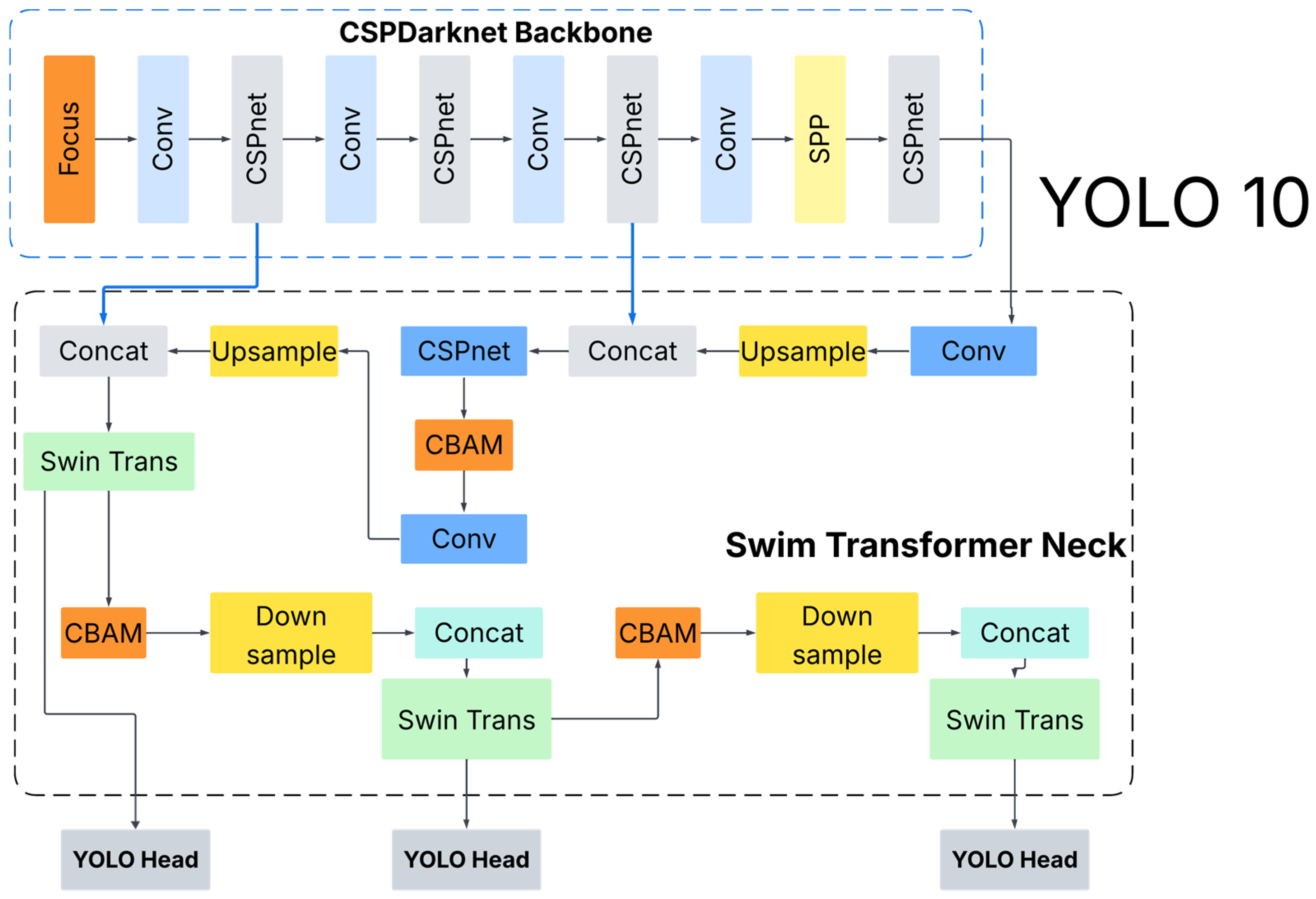
YOLOv10 is released in several variants (n, s, m, b, l, x) and targets post-processing bottlenecks that limited end-to-end latency in prior YOLO versions. It reduces computational redundancy by adopting an NMS-free training/inference strategy and improves gradient flow with an enhanced CSPNet Backbone. The architecture uses dual heads: a one-to-many head during training to strengthen supervision and a one-to-one head at inference for object-level predictions without external NMS.

As summarized in Figure 10, the Backbone integrates an improved CSPNet to enhance gradient flow and reduce redundancy [47]. The Neck employs PAN (Path Aggregation Network) layers for multi-scale feature fusion.

The One-to-Many Head supports multiple predictions per object to improve label assignment during training, while the One-to-One Head enables NMS-free deployment, yielding improved accuracy–latency characteristics.

2.3.4. YOLOv11

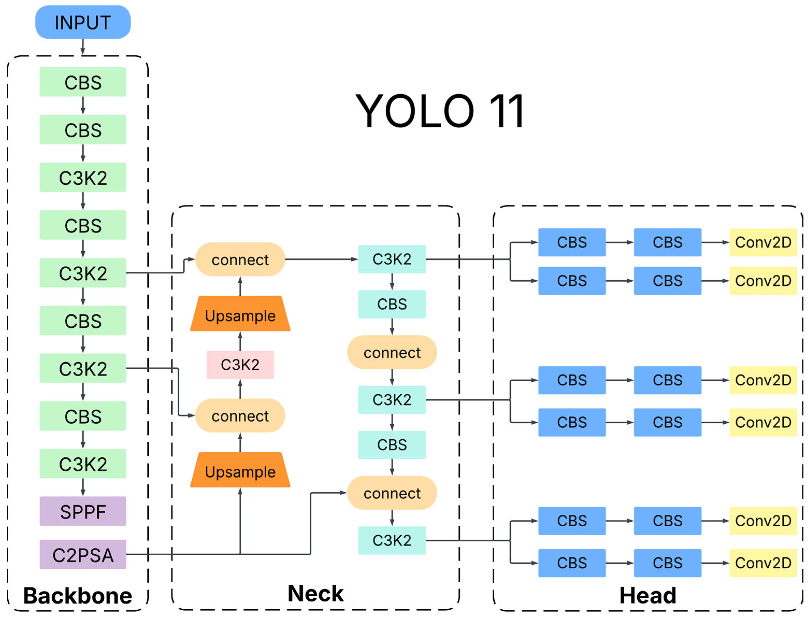
YOLOv11 [47,50,51] introduces architectural refinements that improve compatibility with cloud platforms and NVIDIA-GPU systems, while increasing accuracy (mAP) with fewer parameters. The design adopts PANet (Path Aggregation Network) in the neck for multi-scale feature aggregation.

It employs C3k2 blocks to enhance feature extraction in the Backbone and uses two CSP (Cross-Stage Partial) modules placed before the C2PSA blocks to alleviate bottlenecks and improve gradient flow. These modules operate independently and subsequently concatenate features (see Figure 11).

YOLOv11 models are memory-efficient during both training and inference, facilitating deployment on dedicated hardware and real-time pipelines. They support exports to ONNX, TensorRT, CoreML, and TFLite.

2.3.5. YOLOv12

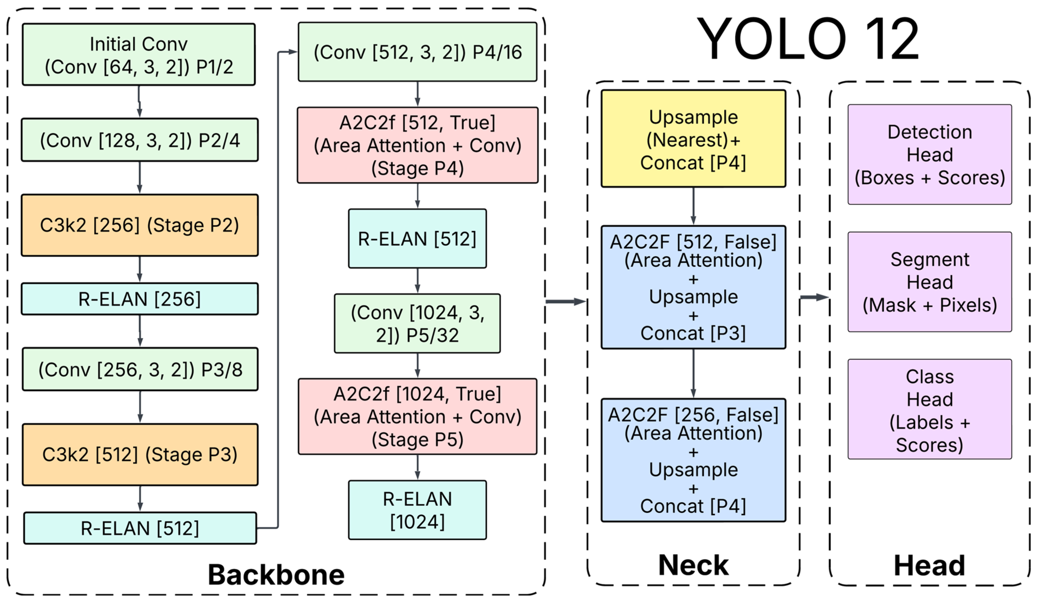
YOLOv12 [52,53,54] adopts a Residual-ELAN (R-ELAN) architecture derived from ELAN to address optimization challenges in large-scale models. It introduces residual connections (akin to layer scaling), together with feature aggregation mechanisms that function similarly to bottleneck designs. The architecture leverages FlashAttention to reduce memory overhead. Additionally, the MLP ratio in attention blocks is lowered (e.g., to 1–2 rather than the typical 4) to reduce computation in the attention layers. It also incorporates separable 7 × 7 convolutions (often referred to as a position perceptor) to implicitly encode positional information (see Figure 12).

A notable limitation is the higher computational cost; exploiting the model’s full potential typically requires GPUs compatible with FlashAttention. Nevertheless, YOLOv12 provides broad task coverage, including object detection, instance segmentation, image classification, pose estimation, and oriented object detection (OBB).

3. Results

This section reports 10 training runs, 5 per methodological stage (see Figure 5). We evaluate five YOLO versions (v8m–v12m). For each stage, we conduct hyperparameter ablation studies and select the best-performing configuration per model for subsequent comparison. Stage 1 addresses traffic light detection, and Stage 2 addresses state recognition (green/yellow/red). After completing all runs, we compare results per model and across configurations to identify the optimal baseline for each version.

All experiments were conducted on a laptop running Windows 11 Home, equipped with an Intel^® Core™ i9-14900HX (2.2 GHz base; Intel Corp., Ho Chi Minh, Vietnam) CPU, an NVIDIA^® GeForce RTX™ 4070 (8 GB GDDR6; NVIDIA Corp., Santa Clara, CA, manufactured in Tainan, Taiwan) GPU, 32 GB DDR5 RAM (SK Hynix Inc., Icheon, Republic of Korea), and a 1 TB NVMe PCIe SSD (Samsung Electronics, Suwon, Republic of Korea). The software stack comprised Conda 23.1.0+, Python 3.10.12, CUDA 12.4, PyTorch 2.5.1+cu121, and Ultralytics 8.3.22.

3.1. Traffic Light Detection (Stage 1) and Traffic Light State Recognition (Stage 2)

The process is divided into two stages: Stage 1 is responsible for detecting traffic lights within the scene, while Stage 2 classifies their operational state (green, yellow, or red). For both stages, five versions of YOLO (v8m through v12m) were trained under the conditions detailed below, and their corresponding performance results are presented in this section.

3.1.1. Hyperparameters for Traffic Light Detection and Traffic Light State Classification

Table 3. Hyperparameters for traffic light detection and traffic light state recognition.

YOLO Model	Hyper-Parameters
	Epochs	Patience	Pretrained	Image Size	lr0	lrf	Batch	Dropout	Batch Size (Step 1: Detection)	Batch Size (Step 2: State)
YOLOv8	500	100	True	640	0.01	0.01	14	0.0	14	10
YOLOv9	500	100	True	640	0.01	0.01	6	0.0	6	10
YOLOv10	500	100	True	640	0.01	0.01	10	0.0	10	8
YOLOv11	500	100	True	640	0.01	0.01	6	0.0	6	8
YOLOv12	500	100	True	640	0.01	0.01	10	0.0	10	8

lists the models and hyperparameters used for Stage 1 and Stage 2. Most default values were retained; however, for both stages, the batch size was varied to examine its effect on the optimization dynamics. As is well established, batch size determines the number of images processed per iteration, influencing convergence speed, gradient noise levels, and generalization capability. Consequently, this parameter was adjusted to stabilize training and maximize detection quality. No explicit regularization (e.g., Dropout) was applied (Dropout = 0.0).

To ensure a fair comparison across YOLOv8–YOLOv12, we adhered to the following normalization practices:

• Same dataset, augmentations, and preprocessing across models.
• Aligned training configuration: epochs, patience, pretrained weights, input size (640), lr0, and lrf.
• Identical validation protocol (holdout split), metrics, and evaluation code path.
• Same input resolution during training and validation.
• Same hardware and software stack.
• Same learning-rate scheduler (cosine decay with lrf = 0.01).

Additionally, we scaled the initial learning rate (lr0) with batch size and adjusted epochs and patience proportionally to approximately preserve the total number of optimization steps. This protocol reduces artificial sensitivity attributable to batch size and lr0, so that observed differences more faithfully reflect architectural effects rather than training-regime artifacts. We kept critical hyperparameters fixed across models (dataset, augmentations, pretrained weights, input size, scheduler, validation protocol, and metrics). As in Step 1, the reported batch size for each model corresponds to the value that achieved the best generalization after a small batch sweep. While Accuracy and Precision remained consistently high across models, results indicate moderate sensitivity to batch size (8 vs. 10), reflecting expected changes in gradient stability; nevertheless, color classification remained stable across illumination conditions.

Note on batch selection. Although we sought to minimize hyperparameter-induced bias, we experimented with batch size and reported for each model the configuration that achieved the best generalization under varying illumination. Because batch size directly affects gradient stability and optimization dynamics, residual performance differences may reflect both model architecture and training regime. We did not apply additional cross-model normalization strategies (e.g., enforcing identical effective batch size via gradient accumulation or strict proportional LR scaling across all settings). Therefore, a fraction of the observed variability may stem from batch-related effects rather than architecture alone.

3.1.2. Performance Evaluation Calculation

The results reported in this paper are derived from the confusion matrices computed for each model. We evaluate Recall (R), Accuracy (A), Precision (P), and Specificity (TNR). In addition, we inspect the F1-score vs. the confidence curve to assess the F1-score at the selected operating threshold. Finally, we report mean Average Precision (mAP) including mAP@0.50 and mAP@0.50–0.95 for each class when applicable.

Let TP, TN, FP, and FN denote true positives, true negatives, false positives, and false negatives, respectively. The metrics are defined as follows:

$$Recall\left(R\right)={\displaystyle \frac{TP}{TP+FN}}$$

(1)

$$Accuracy(Acc.)={\displaystyle \frac{TP+TN}{TP+FN+TN+FP}}$$

(2)

$$Specificity\left(S\right)={\displaystyle \frac{TN}{TN+FP}}$$

(3)

$$Precision\left(P\right)={\displaystyle \frac{TP}{TP+FP}}$$

(4)

$$F1\text{-}Score={\displaystyle \frac{2(R\times R)}{R+P}}$$

(5)

Note. mAP@0.50–0.95 is the mean AP averaged over IoU thresholds 0.50:0.05:0.95; mAP@0.50 is computed at a single threshold (IoU = 0.50).

3.1.3. Results of Traffic Light Detection

Table 4. Traffic light detection performance metrics.

YOLO Model	Class	A	P	R	F1-Score	mAP50	mAP5-95
YOLOv8	traffic_light	0.91	0.963	0.907	0.935	0.944	0.756
YOLOv9	traffic_light	0.93	0.981	0.902	0.940	0.957	0.883
YOLOv10	traffic_light	0.92	0.980	0.915	0.946	0.957	0.812
YOLOv11	traffic_light	0.92	0.947	0.907	0.926	0.941	0.843
YOLOv12	traffic_light	0.91	0.982	0.924	0.952	0.963	0.892

summarizes the performance of the five YOLO versions (v8–v12) trained for the traffic light detection task. The columns report the YOLO version, Class, A (Accuracy), P (Precision), R (Recall), F1-score, mAP@0.50, and mAP@0.50–0.95.

Overall, all YOLO variants achieve high performance, with minor variations across metrics. YOLOv12 attains the highest scores in five of the six metrics, emerging as the best-performing model for traffic light detection, with Accuracy = 0.91, Precision = 0.98, and Recall = 0.92.

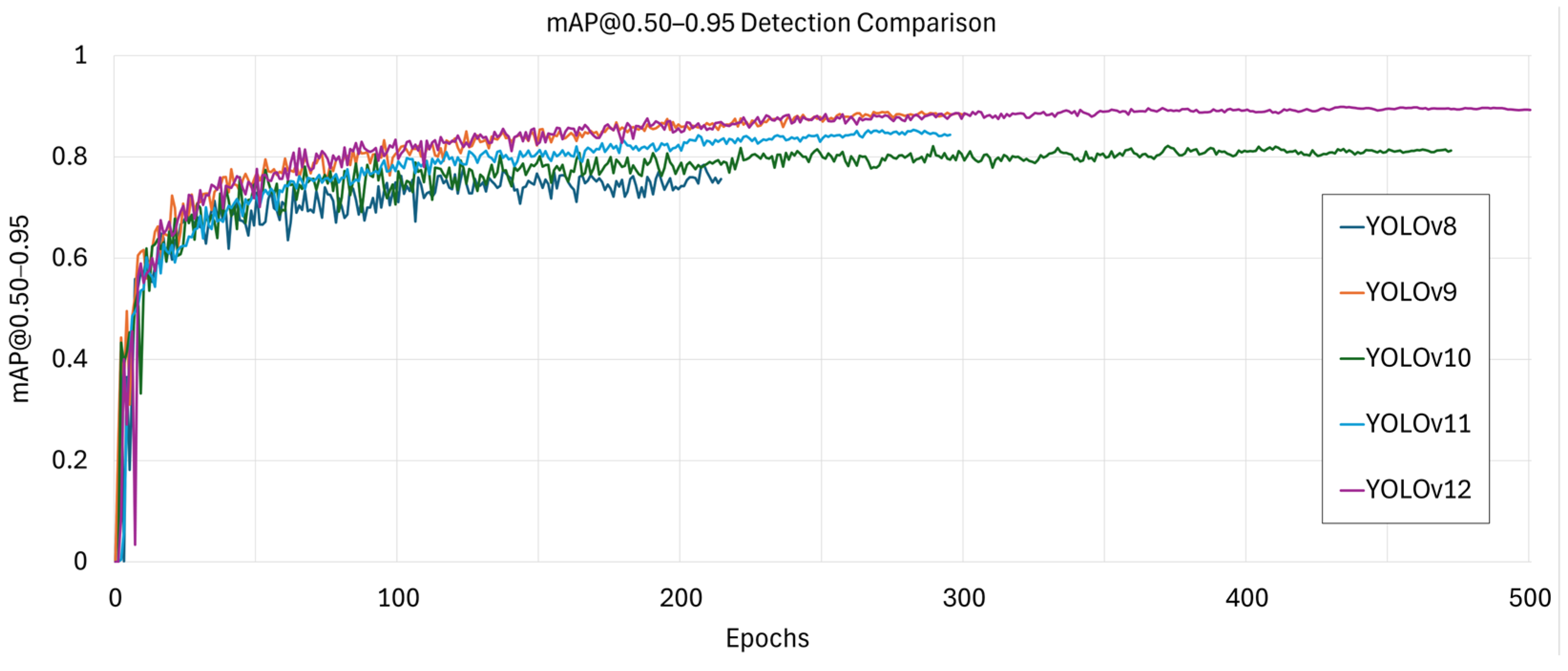
Figure 13 plots mAP@0.50–0.95 vs. epochs, showing consistent improvements during training. YOLOv12 (purple curve) reaches the highest value, followed by YOLOv11 (red), whereas YOLOv8 records the lowest value at the end of training. As the number of epochs increases, the curves converge, suggesting stabilization of performance.

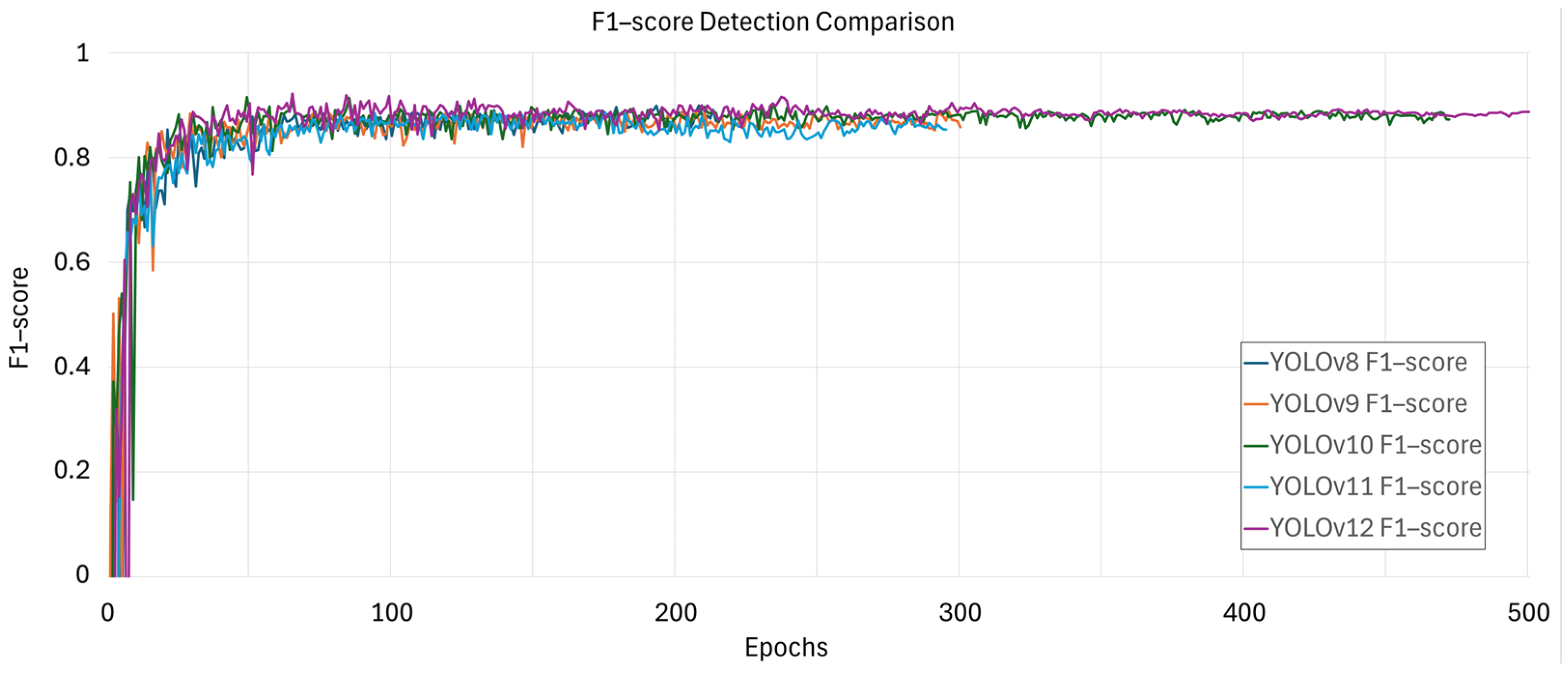
Figure 14 presents the F1-score trajectories across epochs for each YOLO version. Values range from 0 to 1; a higher F1-score indicates a better balance between Precision and Recall at the selected operating threshold.

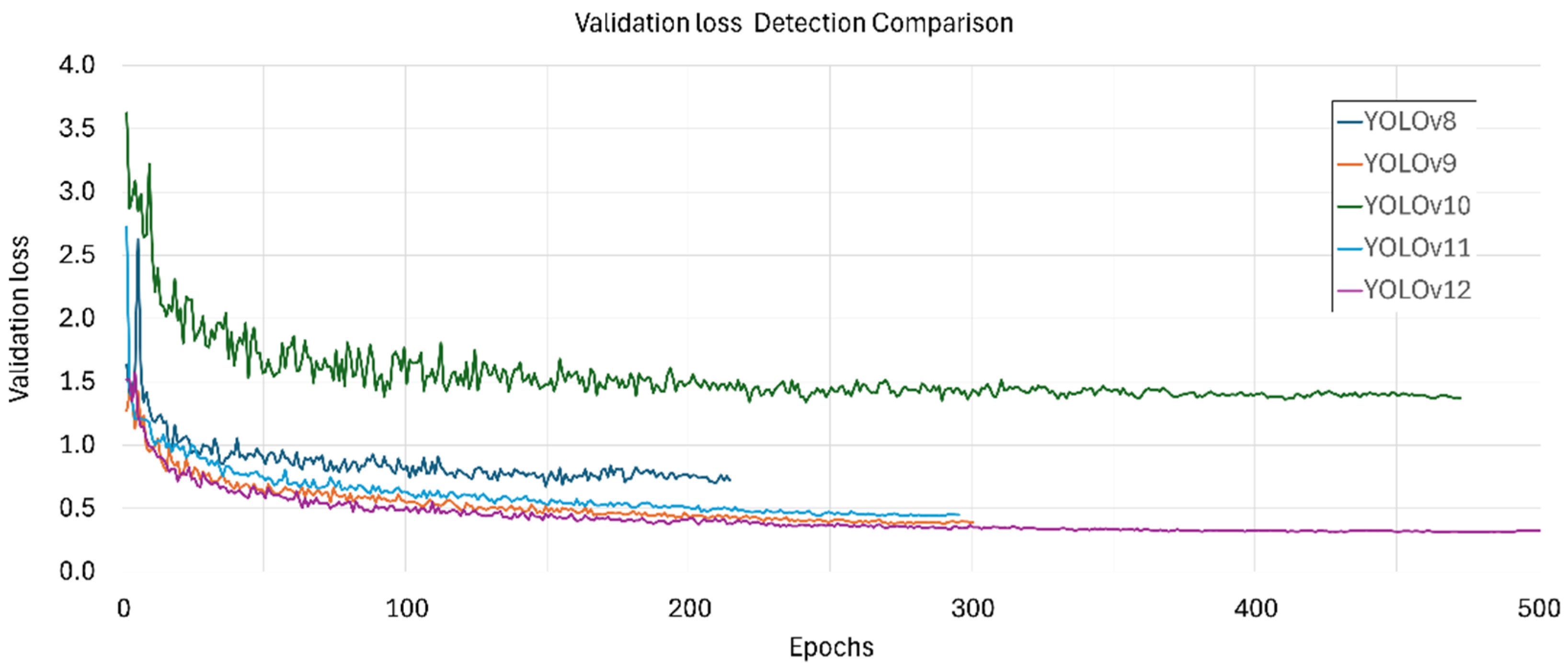
Figure 15 shows the validation loss over epochs, illustrating generalization behavior. YOLOv12 demonstrates the most consistent generalization, whereas YOLOv10 exhibits larger fluctuations. This variability may be linked to its NMS-free training/inference regime, suggesting that further hyperparameter ablation could be beneficial.

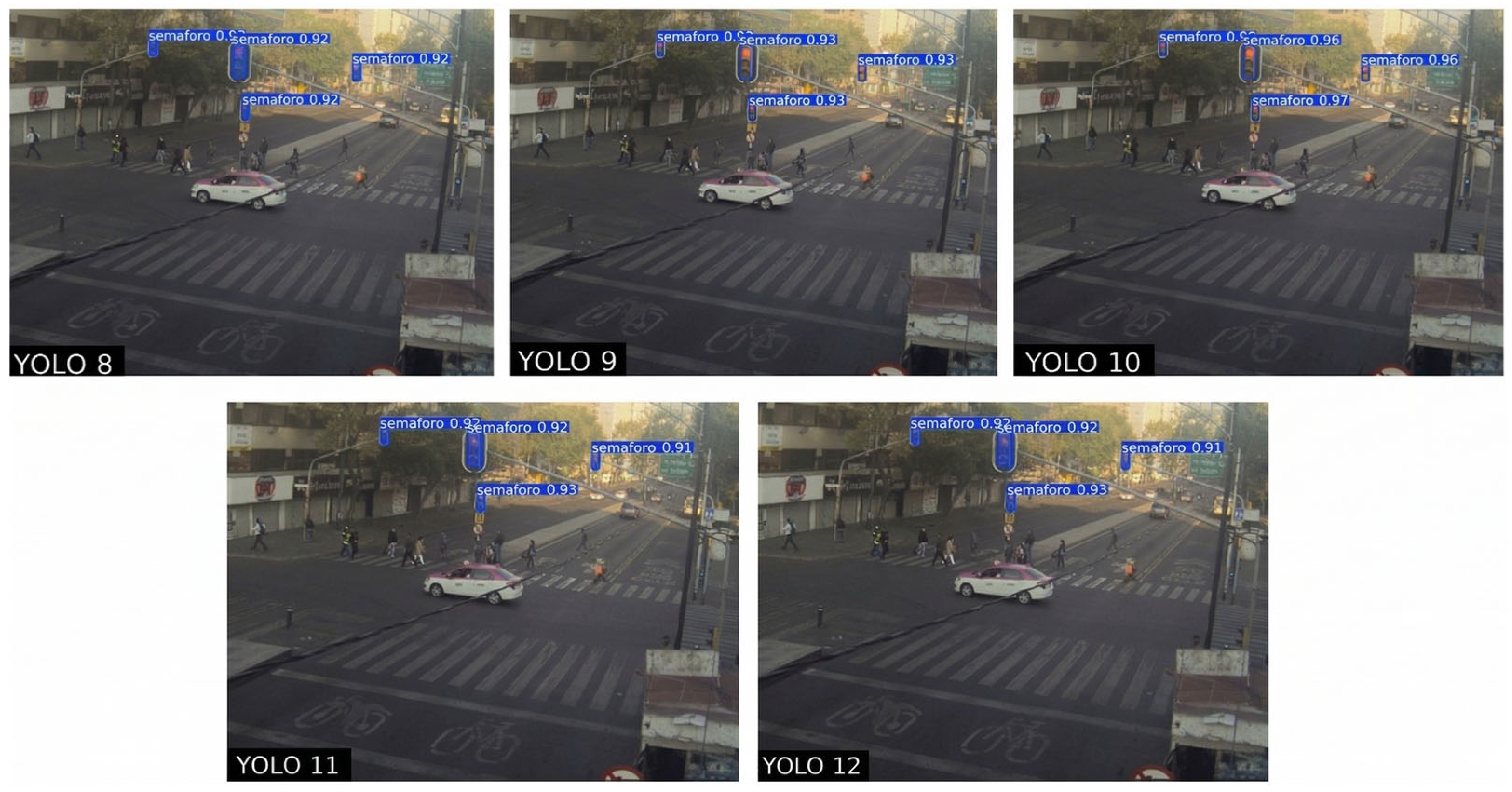
Figure 16 presents qualitative results for the five networks trained for simultaneous multi-instance detection of traffic lights at intersections in Mexico City under real-world conditions; the image is drawn from the 500-image real-time set (see Figure 5). Evaluating all trained networks on the same image reveals their operational behavior beyond aggregate plots.

All five networks correctly detected every traffic light in the scene, each with confidence scores ≥ 0.90. YOLOv10 produced the highest confidence across the four traffic lights (≈0.96–0.97, predominantly 0.97). In contrast, YOLOv8, YOLOv9, YOLOv11, and YOLOv12 yielded confidence scores that were 0.01–0.02 lower on this image, with none exceeding 0.95.

3.1.4. Results of Traffic Light State Recognition

Table 5. Performance metrics for traffic light state recognition (green, yellow, red).

YOLO Model	Class	A	P	R	F1-Score	mAP50	mAP5-95
YOLOv8	trafficlight_green	0.98	0.99	0.993	0.993	0.993	0.869
	trafficlight_yellow	0.99	0.99	0.993	0.993	0.993	0.869
	trafficlight_red	1.00	0.99	0.993	0.993	0.993	0.869
YOLOv9	trafficlight_green	0.98	0.998	0.990	0.994	0.992	0.868
	trafficlight_yellow	1.00	0.998	0.990	0.994	0.992	0.868
	trafficlight_red	1.00	0.998	0.990	0.994	0.992	0.868
YOLOv10	trafficlight_green	0.98	0.993	0.993	0.993	0.994	0.864
	trafficlight_yellow	1.00	0.993	0.993	0.993	0.994	0.864
	trafficlight_red	0.99	0.993	0.993	0.993	0.994	0.864
YOLOv11	trafficlight_green	0.98	0.996	0.993	0.995	0.993	0.869
	trafficlight_yellow	1.00	0.996	0.993	0.995	0.993	0.869
	trafficlight_red	1.00	0.996	0.993	0.995	0.993	0.869
YOLOv12	trafficlight_green	0.98	0.998	0.993	0.996	0.994	0.868
	trafficlight_yellow	0.99	0.998	0.993	0.996	0.994	0.868
	trafficlight_red	1.00	0.998	0.993	0.996	0.994	0.868

indicates that all models achieved high performance, with several reaching values near 1.00. In particular, Recall and F1-score were nearly perfect in multiple cases. Despite the three-class nature of the task, all models successfully identified each traffic light state.

Figure 17 shows rapid improvements during early epochs for all models, indicating a strong ability to focus on the region of interest.

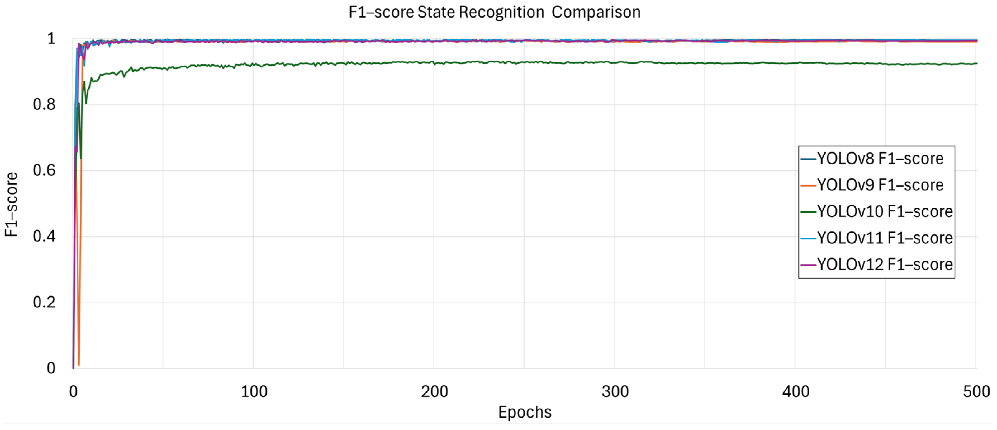
The F1-score trajectories (Figure 18) corroborate the above: curves stabilize with minimal inter-model differences, suggesting that all models learned to identify the region of interest and maintain a balanced Precision–Recall trade-off.

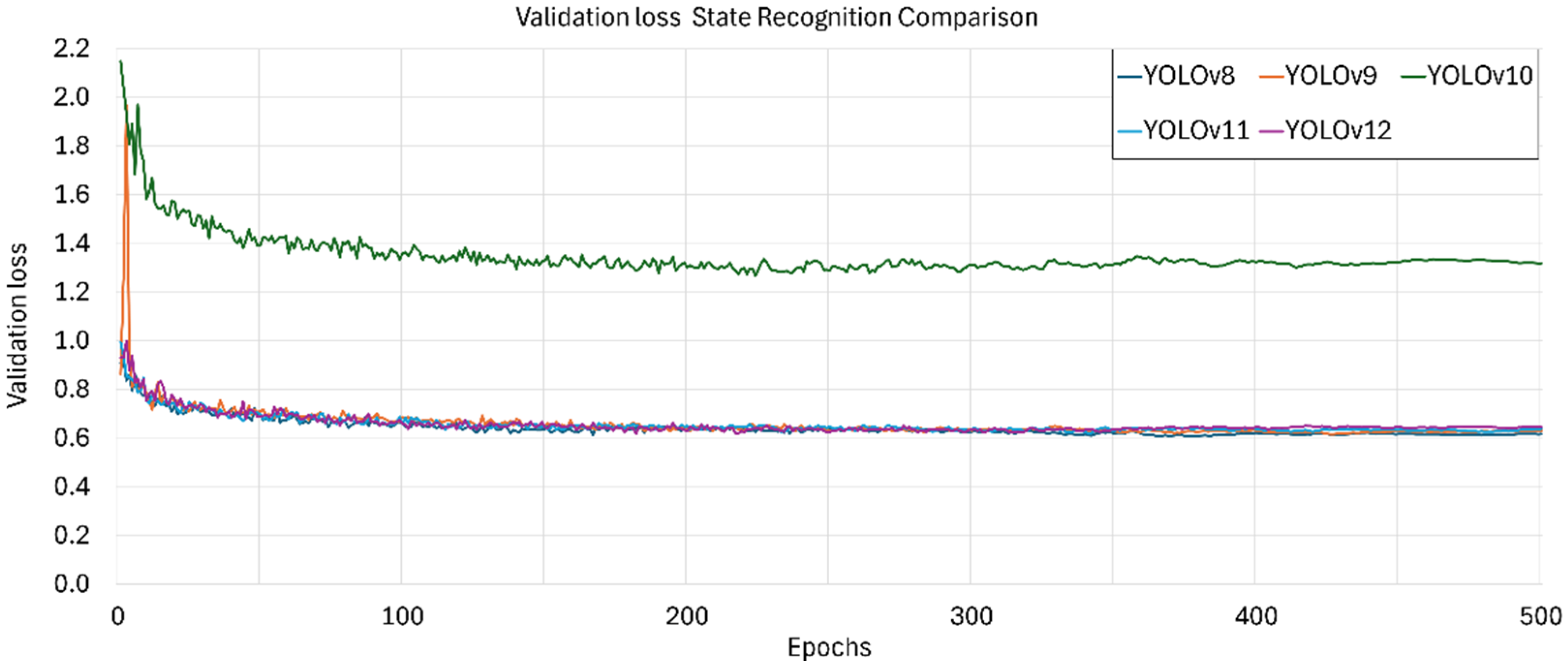
Although earlier plots show minimal fluctuations, Figure 19 reveals that YOLOv10 behaved differently prior to stabilization, indicating initial generalization issues under its default configuration. In contrast, the remaining models reached a stable value toward the end of training, with no significant late-epoch improvements.

3.2. Summary of Findings

3.2.1. Comparative Analysis of YOLO Models

To facilitate the technical comparison,

Table 6. Comparative analysis of models considering inference time.

YOLO Model	mAP50-95 Step 1: Detection	mAP50-95 Step 2: State *	Inference Time (ms) Step 1: Detection	Inference Time (ms) Step 2: State	Loss Stability
YOLOv8	0.756	0.869	14.04	20.28	Medium (Initial Fluctuations)
YOLOv9	0.883	0.868	13.22	24.52	High
YOLOv10	0.812	0.864	11.90	13.42	Very High (More Stable)
YOLOv11	0.843	0.869	12.92	18.66	High
YOLOv12	0.892	0.868	12.90	21.91	High

* Note: The mAP50–95 value for the state classification corresponds to the average across the three classes (green, yellow, red).

summarizes the most relevant findings obtained in both stages of the methodology. In the Detection phase (Step 1), the YOLOv12 model emerged as the most robust architecture, achieving an accuracy of 98.2% and a mAP50–95 of 0.892, representing a substantial improvement over YOLOv8 (mAP50–95 of 0.756). This gain suggests that the optimizations introduced in the most recent versions, particularly in the feature extraction modules and attention mechanisms, significantly enhance performance in visually complex urban environments.

In the State Recognition phase (Step 2), which focused on identifying the traffic light color (green, yellow, red), all evaluated models exhibited outstanding metrics, with F1-score and Recall values approaching 1.00. However, YOLOv10 demonstrated the highest stability and consistency across all three classes, especially in the accurate identification of the “yellow” state, where it slightly outperformed the other versions.

Regarding computational performance, YOLOv10 also emerged as the most efficient model, achieving the lowest inference times in both stages (11.90 ms in detection and 13.42 ms in classification). This performance contrasts with YOLOv9, which, despite offering high accuracy, showed the greatest delay in state classification, with an inference time of 24.52 ms.

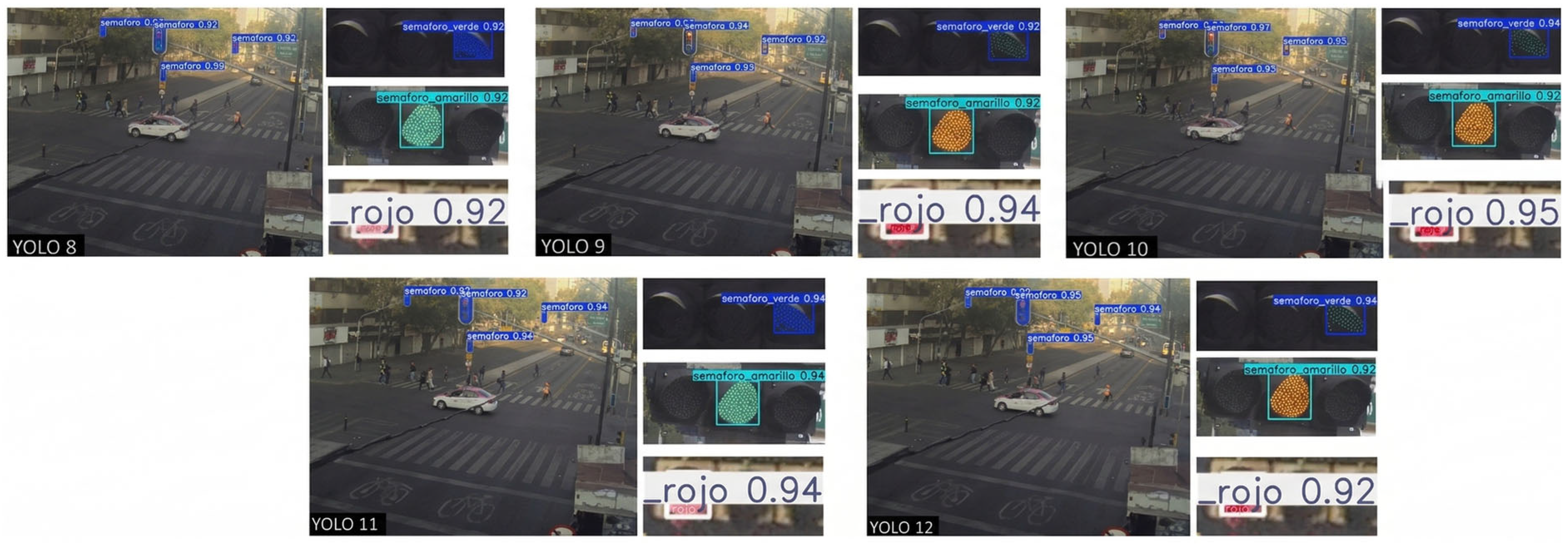
Figure 20 presents the qualitative results obtained from the five architectures trained for the simultaneous detection of multiple traffic light instances and the estimation of their operational state in urban intersections of Mexico City under real-world conditions. The analyzed image originates from the real-time evaluation set, composed of 500 images (see Figure 5). Evaluating all networks on the same scene enables a direct observation of their operational behavior beyond aggregated metrics.

All five architectures correctly identified each traffic light present in the scene, achieving confidence scores of ≥0.90. Among them, YOLOv10 produced the highest confidence scores across the four traffic lights, with values ranging from 0.96 to 0.97 (predominantly 0.97). In contrast, YOLOv8, YOLOv9, YOLOv11, and YOLOv12 yielded confidence scores that were 0.01 to 0.02 lower for this image, with none exceeding 0.95.

In the second evaluation step (state recognition), a visual convergence in model performance is observed: all versions correctly identified the color state of each traffic light with a high level of reliability. This qualitative validation confirms that although precision metrics among the more recent versions are comparable, YOLOv10 exhibits a marginal advantage in detection robustness, reflected in the higher stability and magnitude of its confidence scores.

3.2.2. Evaluation of Overfitting

• Step 1. Traffic Light Detection

To assess the presence of overfitting in the YOLOv8–YOLOv12 models during Step 1, the mAP@0.50–0.95, F1-score, and validation loss curves obtained over 500 training epochs were analyzed. These three metrics allow for identifying divergences between training and validation behavior, which constitute the characteristic indicator of overfitting.

First, the mAP@0.50–0.95 curves (see Figure 13) exhibited a sustained increase during the first 50 epochs, reaching values close to 0.80 for all versions. Subsequently, the mAP stabilized without showing late-epoch degradation:

• YOLOv12 achieved the highest value, with an mAP of approximately 0.88–0.89.
• YOLOv9 and YOLOv11 converged between 0.82 and 0.85.
• YOLOv10, although less accurate, maintained a consistent mAP of around 0.78 without regressions throughout the epochs.

This stability indicates that none of the models experience a loss of generalization capability, since the validation metric does not decrease in the later stages of training. Consistently, the F1-score (see Figure 14) exhibited stable behavior across all models. After the initial convergence observed during the first ~20 epochs, all versions maintained F1 values between 0.85 and 0.90 during the remaining 480 epochs. No abrupt drops or progressive degradation were observed, confirming a stable Precision–Recall balance in validation. The small oscillations present in the curves are minimal and attributable to validation batch variability rather than overfitting.

Finally, the most sensitive metric for detecting overtraining, the validation loss (see Figure 15), showed a descending trend followed by a stabilization phase in all configurations. The final loss values were:

• YOLOv12: ~0.30–0.35, the lowest validation error among the models.
• YOLOv9 and YOLOv11: ~0.40–0.55, with smooth trends and no late-epoch increments.
• YOLOv8: ~0.80–0.90, remaining stable after epoch 100.
• YOLOv10: ~1.50–1.70, the highest loss but without progressive increases over the 500 epochs.

Since in none of the cases does the validation loss exhibit a sustained increase—the classic pattern of overfitting, where training loss continues to decrease while validation loss deteriorates—it is concluded that the models are not memorizing the training set. Overall, the stability observed in the mAP, F1-score, and validation loss confirms that none of the evaluated YOLO models show evidence of overfitting, even under prolonged training over 500 epochs. The curves demonstrate healthy convergence and sustained generalization capacity in the traffic light detection task.

• Step 2. Traffic Light State Recognition

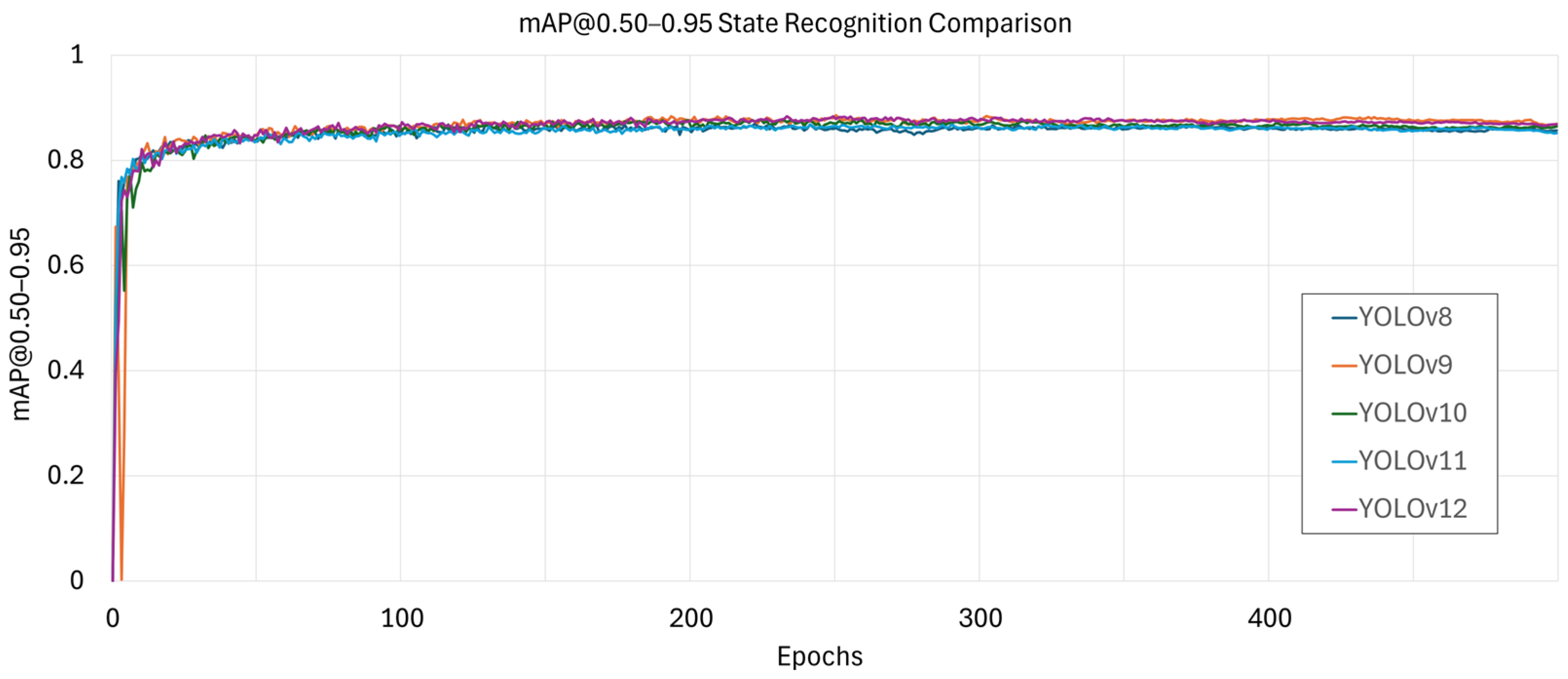
To determine the presence of overfitting in the YOLOv8–YOLOv12 models during Step 2 (traffic light state recognition), the mAP@0.50–0.95, F1-score, and validation loss curves obtained over 500 training epochs were analyzed. As in Step 1, these three metrics allow for detecting divergences between training and validation behavior, which constitute the primary indicator of overfitting. First, the mAP@0.50–0.95 curves (see Figure 17) showed a sharp increase during the first ~20 epochs, reaching values between 0.78 and 0.82 for all YOLO versions. After this initial rise, the mAP stabilized without showing late-epoch decreases:

• YOLOv9 and YOLOv12 reached the highest final values, approximately 0.86.
• YOLOv11 converged around 0.85.
• YOLOv8 and YOLOv10 maintained slightly lower values, around 0.83.

This stability—particularly over the last 400 epochs—indicates that none of the models exhibit a loss of generalization, as the validation metric remains stable without the downward trends characteristic of overfitting. Consistently, the F1-score (see Figure 18) displayed highly stable behavior. After the initial convergence during the first ~10 epochs, YOLOv8, YOLOv9, YOLOv11, and YOLOv12 maintained F1 values close to 0.97–0.99 for the remainder of the training. YOLOv10 showed a lower but stable F1-score around 0.90–0.92, without degradation across epochs. No abrupt decreases or progressive deterioration were observed, confirming that the Precision–Recall balance remains stable in validation. The small oscillations visible in the curves are attributable to minibatch variability rather than indications of overfitting. Finally, the validation loss (see Figure 19) exhibited a sharp decline during the initial epochs, followed by an extended stabilization phase. The final loss values were:

• YOLOv11: ~0.68, the lowest validation loss observed.
• YOLOv8, YOLOv9 and YOLOv12: ~0.70–0.75, with smooth, stable curves.
• YOLOv10: ~1.30–1.40, the highest loss value, but without progressive increases across the 500 epochs.

In no case did the validation loss exhibit the sustained upward trend typical of overfitting, the scenario in which the training loss continues to decrease while the validation loss increases. Therefore, the models are not memorizing the training data. Overall, the stability observed in mAP, F1-score, and validation loss confirms that none of the YOLO models evaluated exhibit evidence of overfitting during the traffic light state recognition stage, even under prolonged 500-epoch training. All curves display healthy convergence and robust generalization capacity in this phase of the system.

4. Conclusions and Discussion

This work investigated traffic light detection and state recognition (green, yellow, red) under natural illumination variability, benchmarking the five most recent YOLO families (YOLOv8m–YOLOv12m). A hybrid dataset was used, combining the public LISA traffic light dataset with a custom corpus acquired at ten intersections in Mexico City across different times of day, thus reflecting uncontrolled real-world conditions. The study sought to identify the YOLO variant and hyperparameter regime that best address both tasks under challenging lighting.

A two-stage pipeline was adopted. Step 1 performs traffic light detection on full-scene images; the detected regions are cropped. Step 2 performs state recognition on those crops. This decomposition was motivated by preliminary trials (not included here) where single-network joint detection and state classification degraded under illumination shifts and scene clutter; separating the tasks improved stability, generalization, and interpretability of errors.

4.1. Findings for Step 1: Traffic Light Detection

Training configurations were aligned across models (epochs, patience, pretrained weights, input size = 640, lr0, lrf, dropout), while batch size was explored as the principal degree of freedom due to its known impact on gradient noise, convergence, and generalization. Under this regime, YOLOv12 achieved the best aggregate performance, leading in F1 (0.952), mAP@0.50 (0.963), and mAP@0.50–0.95 (0.892), and obtaining the highest Precision (0.982) and Recall (0.924) among the compared models. These results indicate that YOLOv12 combines reliable detection with more precise boxes, which are especially valuable under illumination changes where contour quality often degrades. Although the batch size was not fully normalized across models and the learning rate was kept constant, YOLOv12 consistently dominated the most sensitive metrics, suggesting an intrinsic architectural advantage. Normalizing the effective batch (e.g., via gradient accumulation) and/or scaling the LR with the batch would likely sustain or reinforce its superiority.

4.2. Findings for Step 2: Traffic Light State Recognition

For state recognition, all five YOLO versions exhibited fast initial learning and high stability thereafter, with minor differences among the models. Across the three states, the red class generally achieved the best scores, while green/yellow showed small confidence variations (~0.01–0.05). The models converged steadily, and F1-score trajectories stabilized with minimal divergence, providing evidence that all versions learned to focus on the region of interest and to maintain a balanced Precision–Recall trade-off under changing illumination.

4.3. Real-Time Qualitative Evaluation and Model Behavior

Despite YOLOv12’s leadership in the standard offline metrics, the real-time evaluation (500 in-the-wild images from Mexico City) revealed that YOLOv10 produced the highest predicted confidences (≈0.96–0.97 in the exemplar case) across all three states and for all traffic lights in the scene, whereas the other versions were 0.01–0.02 lower on the same image. This divergence is consistent with the architectural philosophies: YOLOv12, with attention-centric and fusion refinements, prioritizes accuracy (higher mAP, tighter boxes) at a higher compute cost; YOLOv10, with NMS-free inference and dual label assignment, reduces post-processing latency and often yields strong confidence under real-time constraints. In short, YOLOv12 excels in aggregate accuracy/IoU-sensitive metrics, whereas YOLOv10 exhibits operational advantages for edge/real-time deployments.

4.4. Model Suitability for Edge-Based Inference

The joint analysis of the five YOLO models shows that their suitability for deployment on edge platforms critically depends on the balance between accuracy, stability, and inference latency. In this regard, although YOLOv12 achieves the highest mAP@0.50–0.95 value during the detection step (0.892), its longer inference time (12.90 ms for detection and 21.91 ms for classification) limits its performance in scenarios with strict real-time constraints. Conversely, YOLOv10 stands out as the architecture with the greatest potential for embedded deployment, as it records the lowest latencies in both stages (11.90 ms and 13.42 ms) and exhibits the highest training stability (“Very High”). This reflects the advantages of its NMS-free design and its optimized label-assignment strategy, both essential properties for supporting typical edge-hardware optimization processes such as quantization, pruning, and TensorRT conversion. Overall, the results indicate that YOLOv10 offers the best trade-off between accuracy, robustness, and computational efficiency, making it the most suitable preliminary candidate for edge systems. However, this conclusion remains subject to future validation on real embedded hardware, such as Jetson Xavier or Orin, to evaluate the effects of thermal, power, and memory constraints that are not reflected in tests performed within a conventional computing environment.

4.5. Representation Choice: Bounding Boxes Are Sufficient

In both detection and state recognition, bounding boxes proved sufficient and appropriate to represent the object of interest. The rectangular ROI aligns with the rigid, quasi-rectangular morphology of traffic lights, stably capturing position and extent without resorting to polygonal annotation. This choice balances geometric alignment, semantic consistency, IoU stability, and model parsimony (Occam’s razor), lowering annotation and computation costs while maintaining high performance.

4.6. Limitations: Domain Coverage and Generalization

Although the five YOLO models remained stable under illumination variation, such stability does not guarantee full generalization. The hybrid dataset, while balanced by time of day and location, does not fully cover adverse weather and rare conditions (e.g., rain, fog, strong backlight, glare on wet pavement). Given that CNN generalization is strongly tied to dataset breadth and diversity, broader environmental stratification is needed to mitigate domain shift at deployment.

4.7. State of the Art

The proposed work stands out by training with a hybrid dataset (LISA + proprietary captures from Mexico City) and by performing an inter-version performance evaluation of YOLOv8–YOLOv12 on real-time video streams under variable natural lighting conditions, achieving 0.93 in detection and 1.0/1.0/0.98 for state recognition (red/yellow/green). These results match or surpass approaches that incorporate specific architectural enhancements or operate within more restricted domains. Considering Table 1, the studies most comparable to the proposed work are those by Kunekar et al. [37] (0.73 in real-time operation) and Sani et al. [38] (mAP@0.5 = 0.781 in nighttime driving). In contrast, the proposed approach demonstrates greater robustness by covering both daytime and nighttime conditions without specializing in a single illumination regime. Another closely related study is that of Munir and Lin [41], which achieves comparable per-class results and even classifies flashing states through a YOLOv10n + ResNet-18 + LSTM pipeline. In our case, the results reveal a performance comparison across the latest YOLO versions under real-world conditions, showing that careful dataset curation combined with recent YOLO families is sufficient to attain competitive performance.

4.8. Practical Implications and Model Selection

• When latency and deployment constraints on embedded/edge devices dominate, YOLOv10 offers structural advantages (NMS-free, simpler post-processing) and strong confidence in real-time inference. However, further experimentation with different edge platforms is needed to determine its actual performance.
• For production, a tiered strategy is feasible: YOLOv12 as the high-fidelity model and YOLOv10 as a low-latency fallback under tight compute budgets.

4.9. Recommendations and Future Work

• Dataset expansion and stratification. Augment the corpus with weather-stratified data (rain, fog, nighttime glare), multiple viewpoints, and context diversity, while preserving class balance and location-wise group splits to avoid scene leakage.
• Controlled hyperparameter normalization. Equalize effective batch size (e.g., gradient accumulation) and apply LR∝batch scaling. Keep total optimization steps constant across models to isolate architectural effects.
• Calibration-aware evaluation. Report ECE/Brier and PR curves by class; re-tune operating thresholds per deployment scenario (e.g., prioritize Recall in safety-critical contexts).
• Ablations for NMS-free regimes. For YOLOv10, run finer ablation studies (label assignment, confidence matching, loss weighting) to temper early-epoch instability while preserving speed.
• Edge-deployment profiling. Benchmark latency/FPS, VRAM, and power on representative edge hardware (e.g., Jetson Xavier/Orin) to produce a cost–benefit analysis before field deployment.

4.10. Final Statement

Under illumination variability, YOLOv12 delivers the best accuracy–localization profile, while YOLOv10 provides operational efficiency and higher real-time confidence. The two-step pipeline with box-level supervision is adequate for both detection and state recognition of traffic lights, and the hybrid dataset approach improves robustness to real-world conditions. Extending environmental coverage, tightening hyperparameter normalization, and profiling on edge hardware are the immediate next steps toward reliable field deployment.

References

1. TomTom Newsroom. Annual TomTom Traffic Index: Unveiling Data-Driven Insights from over 450 Billion Miles Driven in 2024. 2025. Available online: https://www.tomtom.com/ (accessed on 8 March 2026).
2. World Health Organization. Global Status Report on Road Safety 2023; World Health Organization: Geneva, Switzerland, 2023; Available online: https://www.who.int/publications/i/item/9789240086517 (accessed on 8 March 2026).
3. Secretaría de Comunicaciones y Transportes. Uso del Celular, una de las Principales Causas de Accidentes Viales. 2024. Available online: https://www.gob.mx/sct (accessed on 8 March 2026).
4. Soria, A.G. Concientización y prevención de accidentes viales a través de campañas de seguridad vial. In Proceedings of the XXIVth World Road Congress; Instituto Mexicano del Transporte: Querétaro, Mexico, 2021; Available online: https://proceedings-mexico2011.piarc.org/ressources/files/4/0306-es.pdf (accessed on 8 March 2026).
5. Parekh, D.; Poddar, N.; Rajpurkar, A.; Chahal, M.; Kumar, N.; Joshi, G.P.; Cho, W. A review on autonomous vehicles: Progress, methods and challenges. Electronics 2022, 11, 2162. [Google Scholar] [CrossRef]
6. Hasanujjaman, M.; Chowdhury, M.Z.; Jang, Y.M. Sensor fusion in autonomous vehicle with traffic surveillance camera system: Detection, localization, and AI networking. Sensors 2023, 23, 3335. [Google Scholar] [CrossRef] [PubMed]
7. National Highway Traffic Safety Administration (NHTSA). Traffic Safety Facts 2021: A Compilation of Motor Vehicle Traffic Crash Data; U.S. Department of Transportation: Washington, DC, USA, 2023. Available online: https://rosap.ntl.bts.gov/view/dot/78020/dot_78020_DS1.pdf (accessed on 8 March 2026).
8. Alawadhi, M.; Almazrouie, J.; Kamil, M.; Khalil, K.A. A systematic literature review of the factors influencing the adoption of autonomous driving. Int. J. Syst. Assur. Eng. Manag. 2020, 11, 1065–1082. [Google Scholar] [CrossRef]
9. Almaskati, D.; Kermanshachi, S.; Pamidimukkula, A. Autonomous vehicles and traffic accidents. Transp. Res. Procedia 2023, 73, 321–328. [Google Scholar] [CrossRef]
10. Chen, S.; Zong, S.; Chen, T.; Huang, Z.; Chen, Y.; Labi, S. A taxonomy for autonomous vehicles considering ambient road infrastructure. Sustainability 2023, 15, 11258. [Google Scholar] [CrossRef]
11. Kumar, S.; Singh, S.K.; Varshney, S.; Singh, S.; Kumar, P.; Kim, B.-G.; Ra, I.-H. Fusion of DeepSORT and YOLOv5 for effective vehicle detection and tracking in real-time traffic management sustainable system. Sustainability 2023, 15, 16869. [Google Scholar] [CrossRef]
12. Flores-Calero, M.; Astudillo, C.A.; Guevara, D.; Maza, J.; Lita, B.S.; Defaz, B.; Ante, J.S.; Zabala-Blanco, D.; Armingol Moreno, J.M. Traffic sign detection and recognition using YOLO object detection algorithm: A systematic review. Mathematics 2024, 12, 297. [Google Scholar] [CrossRef]
13. Liu, Y.; Luo, P. YOLO-TS: A lightweight YOLO model for traffic sign detection. IEEE Access 2024, 12, 169013–169023. [Google Scholar] [CrossRef]
14. Chauhan, A.; Chorge, O.; Chaudhari, R.; Patil, K.T. A survey paper on intelligent traffic lights. Int. Res. J. Eng. Technol. (IRJET) 2021, 8, 1054–1057. [Google Scholar] [CrossRef]
15. Gautam, S.; Kumar, A. Image-based automatic traffic light detection system for autonomous cars: A review. Multimed. Tools Appl. 2023, 82, 26135–26182. [Google Scholar] [CrossRef]
16. Galvao, L.G.; Abbod, M.; Kalganova, T.; Palade, V.; Huda, M.N. Pedestrian and vehicle detection in autonomous vehicle perception systems—A review. Sensors 2021, 21, 7267. [Google Scholar] [CrossRef] [PubMed]
17. Zakaria, N.J.; Shapiai, M.I.; Ghani, R.A.; Yassin, M.N.M.; Ibrahim, M.Z.; Wahid, N. Lane detection in autonomous vehicles: A systematic review. IEEE Access 2023, 11, 3729–3765. [Google Scholar] [CrossRef]
18. Ghahremannezhad, H.; Shi, H.; Liu, C. Object detection in traffic videos: A survey. IEEE Trans. Intell. Transp. Syst. 2023, 24, 6780–6799. [Google Scholar] [CrossRef]
19. Boukerche, A.; Hou, Z. Object detection using deep learning methods in traffic scenarios. ACM Comput. Surv. 2021, 54, 1–35. [Google Scholar] [CrossRef]
20. Dewi, C.; Chen, R.-C.; Jiang, X.; Yu, H. Deep convolutional neural network for enhancing traffic sign recognition developed on YOLOv4. Multimed. Tools Appl. 2022, 81, 37821–37845. [Google Scholar] [CrossRef]
21. Kumar, K.; Santhosh Reddy, D.; Rajalakshmi, P. 3D YOLO-SM: End-to-end approach for real-time traffic light detection and recognition in complex scenarios. In Proceedings of the 2024 IEEE 100th Vehicular Technology Conference (VTC2024-Fall), Washington, DC, USA, 7–10 October 2024. [Google Scholar] [CrossRef]
22. Pavel, M.I.; Tan, S.Y.; Abdullah, A. Vision-based autonomous vehicle systems based on deep learning: A systematic literature review. Appl. Sci. 2022, 12, 6831. [Google Scholar] [CrossRef]
23. Karakan, A. Detection of red, yellow, and green lights in real-time traffic lights with YOLO architecture. Celal Bayar Univ. J. Sci. 2024, 20, 28–36. [Google Scholar] [CrossRef]
24. Wali, S.B.; Abdullah, M.A.; Hannan, M.A.; Hussain, A.; Samad, S.A.; Ker, P.J.; Mansor, M.B. Vision-based traffic sign detection and recognition systems: Current trends and challenges. Sensors 2019, 19, 2093. [Google Scholar] [CrossRef]
25. Rana, C. Artificial intelligence-based object detection and traffic prediction by autonomous vehicles—A review. Expert Syst. Appl. 2024, 255, 124664. [Google Scholar] [CrossRef]
26. Liang, L.; Ma, H.; Zhao, L.; Xie, X.; Hua, C.; Zhang, M.; Zhang, Y. Vehicle detection algorithms for autonomous driving: A review. Sensors 2024, 24, 3088. [Google Scholar] [CrossRef]
27. Karangwa, J.; Liu, J.; Zeng, Z. Vehicle detection for autonomous driving: A review of algorithms and datasets. IEEE Trans. Intell. Transp. Syst. 2023, 24, 11568–11594. [Google Scholar] [CrossRef]
28. Liu, M.; Yurtsever, E.; Fossaert, J.; Zhou, X.; Zimmer, W.; Cui, Y.; Zagar, B.L.; Knoll, A.C. A survey on autonomous driving datasets: Statistics, annotation quality, and a future outlook. IEEE Trans. Intell. Veh. 2024, 9, 7138–7164. [Google Scholar] [CrossRef]
29. Song, Z.; He, Z.; Li, X.; Ma, Q.; Ming, R.; Mao, Z.; Pei, H.; Peng, L.; Hu, J.; Yao, D.; et al. Synthetic datasets for autonomous driving: A survey. IEEE Trans. Intell. Veh. 2024, 9, 1847–1864. [Google Scholar] [CrossRef]
30. Zhao, R.; Tang, S.H.; Shen, J.; Supeni, E.E.B.; Rahim, S.A. Enhancing autonomous driving safety: A robust traffic sign detection and recognition model TSD-YOLO. Signal Process. 2024, 225, 109619. [Google Scholar] [CrossRef]
31. Ayegbusi, O.A.; Akinwumi, A.O.; Ogbeide, O.; Akingbesote, A.O.; Obafemi, J.R.; Akinrolabu, O.D.; Rotiba, O. A deep learning-based model for traffic signal control using the YOLO algorithm. Int. J. Comput. Appl. 2025, 186, 43–54. [Google Scholar] [CrossRef]
32. Pavlitska, S.; Lambing, N.; Bangaru, A.K.; Zöllner, J.M. Traffic light recognition using convolutional neural networks: A survey. In Proceedings of the 2023 IEEE 26th International Conference on Intelligent Transportation Systems (ITSC), Bilbao, Spain, 24–28 September 2023. [Google Scholar] [CrossRef]
33. Yang, L.; He, Z.; Zhao, X.; Fang, S.; Yuan, J.; He, Y.; Li, S.; Liu, S. A deep learning method for traffic light state recognition. J. Intell. Connect. Veh. 2023, 6, 173–182. [Google Scholar] [CrossRef]
34. Yoneda, K.; Ichihara, N.; Kawanishi, H.; Okuno, T.; Cao, L.; Suganuma, N. Sun-glare region recognition using visual explanations for traffic light detection. In Proceedings of the 2021 IEEE Intelligent Vehicles Symposium (IV), Nagoya, Japan, 11–17 July 2021. [Google Scholar] [CrossRef]
35. Wang, Q.; Zhang, Q.; Liang, X.; Wang, Y.; Zhou, C.; Mikulovich, V.I. Traffic lights detection and recognition method based on the improved YOLOv4 algorithm. Sensors 2021, 22, 200. [Google Scholar] [CrossRef]
36. Song, J.; Hu, T.; Gong, Z.; Zhang, Y.; Cui, M. TLDM: An enhanced traffic light detection model based on YOLOv5. Electronics 2024, 13, 3080. [Google Scholar] [CrossRef]
37. Kunekar, P.; Narule, Y.; Mahajan, R.; Mandlapure, S.; Mehendale, E.; Meshram, Y. Traffic management system using YOLO algorithm. Eng. Proc. 2024, 59, 210. [Google Scholar] [CrossRef]
38. Sani, Z.M.; Saari, M.I.F.; Izzudin, T.A. Traffic light (circle) detection and recognition using YOLO and image processing technique. In Proceedings of the 6th International Conference on Electrical, Control and Computer Engineering (InECCE2021), Kuantan, Malaysia, 23 August 2021. [Google Scholar] [CrossRef]
39. Sarhan, N.H.; Al-Omary, A.Y. Traffic light detection using OpenCV and YOLO. In Proceedings of the 2022 International Conference on Innovation and Intelligence for Informatics, Computing, and Technologies (3ICT), Sakheer, Bahrain, 20–21 November 2022. [Google Scholar] [CrossRef]
40. Ma, Y.; Arifah, F.; Afifah, Q.; Bun, L.; Zhang, K.; Tang, M. Traffic light recognition assistant for color vision deficiency using YOLO with multilingual audio feedback. Sensors 2026, 26, 1093. [Google Scholar] [CrossRef]
41. Munir, S.; Lin, H.-Y. LNT-YOLO: A lightweight nighttime traffic light detection model. Smart Cities 2025, 8, 95. [Google Scholar] [CrossRef]
42. Tammisetti, V.; Stettinger, G.; Cuellar, M.P.; Molina-Solana, M. Meta-YOLOv8: Meta-learning-enhanced YOLOv8 for precise traffic light color detection in ADAS. Electronics 2025, 14, 468. [Google Scholar] [CrossRef]
43. Yagob, F.; Sasiadek, J.Z. Enhanced real-time method traffic light signal color recognition using advanced convolutional neural network techniques. World Electr. Veh. J. 2025, 16, 441. [Google Scholar] [CrossRef]
44. Khaled, L.B.; Rahman, M.; Ebu, I.A.; Ball, J.E. FlashLightNet: An end-to-end deep learning framework for real-time detection and classification of static and flashing traffic light states. Sensors 2025, 25, 6423. [Google Scholar] [CrossRef]
45. Redmon, J.; Divvala, S.; Girshick, R.; Farhadi, A. You only look once: Unified, real-time object detection. In Proceedings of the IEEE Conference on Computer Vision and Pattern Recognition (CVPR), Las Vegas, NV, USA, 27–30 June 2016; pp. 779–788. Available online: https://www.cv-foundation.org/openaccess/content_cvpr_2016/html/Redmon_You_Only_Look_CVPR_2016_paper.html (accessed on 8 March 2026).
46. Lin, M.; Chen, Q.; Yan, S. Network in network. arXiv 2013, arXiv:1312.4400. [Google Scholar] [CrossRef]
47. Jocher, G.; Chaurasia, A.; Qiu, J. Ultralytics YOLOv8. 2023. Available online: https://docs.ultralytics.com/models/yolov8/ (accessed on 8 March 2026).
48. Yaseen, M. What is YOLOv9: An in-depth exploration of the internal features of the next-generation object detector. arXiv 2024, arXiv:2409.07813. [Google Scholar] [CrossRef]
49. Wang, C.-Y.; Yeh, I.-H.; Liao, H.-Y.M. YOLOv9: Learning what you want to learn using programmable gradient information. arXiv 2024, arXiv:2402.13616. [Google Scholar] [CrossRef]
50. Khanam, R.; Hussain, M. YOLOv11: An overview of the key architectural enhancements. arXiv 2024, arXiv:2410.17725. [Google Scholar] [CrossRef]
51. Rasheed, A.F.; Zarkoosh, M. YOLOv11 optimization for efficient resource utilization. arXiv 2024, arXiv:2412.14790. [Google Scholar] [CrossRef]
52. Alif, M.A.R.; Hussain, M. YOLOv12: A breakdown of the key architectural features. arXiv 2025, arXiv:2502.14740. [Google Scholar] [CrossRef]
53. Tian, Y.; Ye, Q.; Doermann, D. YOLOv12: Attention-centric real-time object detectors. arXiv 2025, arXiv:2502.12524. [Google Scholar] [CrossRef]
54. Khanam, R.; Hussain, M. A review of YOLOv12: Attention-based enhancements vs. previous versions. arXiv 2025, arXiv:2504.11995. [Google Scholar] [CrossRef]
Figure 1. Example scenario of an advanced driver assistance system (ADAS) detecting traffic lights.
Vehicles 08 00090 g001
Figure 2. Schematic of the main challenges in automatic traffic light detection and state recognition.
Vehicles 08 00090 g002
Figure 3. Example images illustrating representative challenges faced by automatic traffic light detection.
Vehicles 08 00090 g003
Figure 4. Proposed pipeline for traffic light detection and state recognition.
Vehicles 08 00090 g004
Figure 5. Dataset structure, management, and training workflow. Each YOLO variant (v8m, v9m, v10m, v11m, v12m) was trained on Training Set A and validated on Validation Set A. We conducted ablation studies to select task-appropriate hyperparameters for traffic light detection. After achieving stable convergence for each version, we evaluated the models on the real-time test set to quantify performance in the wild.
Vehicles 08 00090 g005
Figure 6. Example images from the LISA dataset and the custom dataset used during the training, validation, and testing phases.
Vehicles 08 00090 g006
Figure 7. Schematic of the YOLOv1 architecture, showing kernel sizes, the number of filters, and strides; repeated blocks are indicated by multiplicity markers (e.g., ×2, ×4).
Vehicles 08 00090 g007
Figure 8. YOLOv8 structure, divided into Backbone, Neck, and Head.
Vehicles 08 00090 g008
Figure 9. YOLOv9 structure showing the integration of reversible functions, PGI, and GELAN.
Vehicles 08 00090 g009
Figure 10. YOLOv10 structure integrating an NMS-free strategy with dual label assignments (one-to-many for training, one-to-one for inference).
Vehicles 08 00090 g010
Figure 11. YOLOv11 structure integrating C3k2 blocks and SPPF (Spatial Pyramid Pooling–Fast) within the Backbone/Neck/Head pipeline.
Vehicles 08 00090 g011
Figure 12. YOLOv12 structure illustrating R-ELAN-based optimization within the Backbone, with FlashAttention and separable 7 × 7 convolutions for positional encoding.
Vehicles 08 00090 g012
Figure 13. mAP@0.50–0.95 vs. epochs in traffic light detection training.
Vehicles 08 00090 g013
Figure 14. F1-score vs. epochs in traffic light detection training.
Vehicles 08 00090 g014
Figure 15. Validation loss vs. epochs during traffic light detection training.
Vehicles 08 00090 g015
Figure 16. Real-time images used to qualitatively evaluate each trained network (traffic light detection, YOLO v8–v12).
Vehicles 08 00090 g016
Figure 17. Learning curves (state recognition): metric trajectories vs. epochs.
Vehicles 08 00090 g017
Figure 18. F1-score vs. epochs in traffic light state recognition.
Vehicles 08 00090 g018
Figure 19. Validation loss vs. epochs in traffic light state recognition.
Vehicles 08 00090 g019
Figure 20. Example predictions for the three traffic light states (green, yellow, red) evaluated with each trained model (YOLO v8–v12).
Vehicles 08 00090 g020