Optimisation-Based Tuning of a Triple-Loop Vehicle Controller to Mimic Professional Driver Performance in a DiL Simulator

Abstract

This paper presents a simulation-based methodology for automated tuning of a triple-loop controller (steering, throttle, and braking) for a Dallara single-seater race car. The approach targets on-track driving at handling limits, where strong nonlinearities and coupled dynamics dominate, treating the vehicle as a black box. Five controller gains are optimized via derivative-free pattern search, using reference trajectories from a professional driver in a Driver-in-the-Loop (DiL) simulator. Human-likeness is promoted by penalty terms on state and control trajectories while maximizing distance over a fixed horizon as a proxy for lap-time reduction. The application uses a high-fidelity multibody vehicle model with realistic tire, suspension, and actuator dynamics in the DiL environment, rather than simplified single-track representations. Contributions are: (i) effective application of derivative-free optimization to complex, high-dimensional, black-box vehicle systems; and (ii) a systematic, reproducible procedure for automatic tuning of controller parameters with a predetermined architecture to reproduce a professional driver’s performance and embed human-likeness. Optimization required approximately 2.4 h. Results show that the optimized controller improves track coverage by 63.6 m (1.1% increase) compared to manual tuning while maintaining a realistic driving style, offering a more systematic and reliable solution than manual, trial-and-error calibration.

1. Introduction

Systematically tuning complex multi-loop controllers for vehicles operating at the limits of handling presents a significant challenge in high-performance vehicle control. At these operating conditions, the vehicle dynamics are highly nonlinear, with strong coupling between lateral and longitudinal subsystems, tire saturation effects, and complex interactions between suspension, aerodynamics, and actuation systems. Traditional manual tuning approaches, while often effective, are time-consuming, require substantial expertise, and struggle to consistently balance competing objectives such as trajectory tracking accuracy, human-likeness, and performance maximization.

In motorsport engineering and high-fidelity simulation applications, controllers must replicate the behavior of skilled human drivers operating vehicles near their dynamic limits, following aggressive trajectories that maximize performance. This requires control architectures with multiple sub-controllers, each responsible for specific actuation systems (braking, acceleration, steering), and each potentially adopting different control strategies (proportional, integral, derivative, or combinations thereof) depending on the subsystem dynamics and desired behavior.

In such scenarios, the controller must act as a virtual driver, capable of replicating complex decision-making and dynamic responses that would normally come from a human operating the vehicle at high speeds. A common approach in this domain involves generating reference trajectories from real driver input—often obtained from hardware-in-the-loop or Driver-in-the-Loop (DiL) simulators—and designing controllers that can reproduce those trajectories with high precision.

To achieve this level of fidelity, the control architecture is often decomposed into multiple sub-controllers, each responsible for a specific actuation system such as braking, acceleration, and steering. These sub-controllers may adopt different control strategies—proportional, integral, derivative, or combinations thereof—depending on the dynamics of the corresponding subsystem and the desired control behavior.

This setting presents unique challenges in terms of control design and tuning, particularly when the goal is to match or exceed human-level driving performance under dynamic conditions.

1.1. Related Work

Trajectory tracking controllers have been widely explored in the context of autonomous and assisted driving, typically relying on simplified vehicle models and targeting standard road conditions rather than high-performance scenarios. In [1], a PD steering controller with speed-dependent look-ahead distance is implemented on a single-track model, assuming constant longitudinal velocity at the front wheel. Similarly, ref. [2] introduces a feedback-feedforward controller incorporating road slope estimation via an optimal control formulation but applies a linear longitudinal model suited for connected, road-going vehicles.

Other works, such as [3], focus on control design for small-scale RC cars using basic linear models identified from data and compare different strategies like PID, MPC, and LQR. In [4], a hybrid controller combines PID, feedforward preview, and LQR control to address both lateral and longitudinal dynamics, again using a single-track model with linear tire assumptions, suitable for non-racing autonomous platforms.

A more detailed tire representation is used in [5], where an ESC system distributes torque among four in-wheel motors to control yaw rate while avoiding tire saturation. Despite the inclusion of a combined-slip tire model, the control is still based on a simplified single-track vehicle structure.

Beyond the design of trajectory tracking controllers, several studies have focused on tuning methodologies to improve control performance, often employing optimization strategies or adaptive mechanisms. These works, while varied in approach, continue to rely on simplified vehicle representations and are not tailored for racing scenarios.

In [6], a PID controller is combined with an adaptive feedforward strategy that adjusts based on lateral deviation, heading error, and road curvature. Although tested on real roads in China, the method is implemented on a single-track vehicle model, limiting its applicability to more complex dynamics. A similar structure is adopted in [7], where the authors employ the Twiddle algorithm to tune a PID controller by minimizing the positional error of the vehicle on a desired path, again using a single-track formulation.

More advanced optimization techniques are explored in [8], where a genetic algorithm is used for the multi-objective tuning of a PID controller governing the rear wing flap angles, with the goal of maximizing downforce and optimizing the lift-to-drag ratio. Despite addressing a racing-relevant component, the control logic is not integrated into a full vehicle dynamics context.

In [9], a fuzzy logic layer is introduced to dynamically tune PID gains based on lateral and heading errors, improving tracking performance on a basic curved path. Likewise, ref. [10] proposes a Human-Simulating Intelligent Control (HSIC) system that adjusts control strategies based on the error magnitude, mimicking different human driving behaviors within a simplified single-track model.

Finally, ref. [11] integrates a single-neuron neural network into a PID tuning process, adapting the controller gains in real time while assuming a fixed longitudinal velocity. As with the other approaches, the model’s simplicity restricts its application to lower-speed or less demanding driving scenarios.

Overall, while these studies demonstrate a broad range of tuning techniques—from heuristic search to machine learning and fuzzy logic—their implementation on low-order vehicle models and lack of integration with high-performance dynamics underscore the gap in addressing the challenges posed by racing or near-limit driving conditions.

Besides the variety of tuning strategies discussed above, a key challenge in controller parameterization arises when the overall closed-loop system, composed of both the vehicle and its controller, cannot be easily expressed in analytical form. In such cases, the system behaves effectively as a black box, making gradient-based optimization impractical. This motivates the use of derivative-free methods such as the patternsearch algorithm, which iteratively explores the search space without requiring explicit model gradients and is particularly well-suited for noisy or highly nonlinear systems.

The patternsearch method has been successfully applied in different engineering domains. For example, in [12] it was used to optimize the dynamic allocation of rectifying weight coefficients in a combined direction control law for a small UAV (Unmanned Aerial Vehicle), integrating differential braking and nose-wheel steering during ground operations. The algorithm efficiently adapted the control strategy to varying speeds, improving stability and directional control without relying on gradient information. In [13], patternsearch was employed for parameter identification of a flexible ring tire model, showing robustness against noisy data and fast convergence, although with the known limitation of being prone to local minima.

Beyond vehicle-related applications, patternsearch has also been adopted in biomechanics and mechanical design. In [14], it was integrated into a bilevel inverse optimal control framework to identify human motor control objectives during walking, enabling efficient multiobjective optimization consistent with experimental gait data. Similarly, ref. [15] applied the algorithm within a multiobjective optimization scheme for spiral bevel gears, balancing conflicting targets such as noise, vibration, and efficiency by efficiently identifying Pareto-optimal solutions.

These works highlight the versatility of patternsearch in addressing nonlinear, noisy, or multiobjective problems across different domains, confirming its value as a robust optimization strategy when conventional gradient-based methods are not applicable.

1.2. Paper’s Contributions

This paper proposes an automated tuning procedure for a high-performance vehicle controller designed for on-track driving. Unlike previous studies that focus on road vehicles or simplified models, the presented approach addresses the challenge of controlling a vehicle operating at the limits of handling, where nonlinearities and complex dynamic interactions play a dominant role.

The tuning process is based on a derivative-free optimization method, Patternsearch, which is particularly suitable for systems provided as black boxes, where the underlying dynamic equations are inaccessible or too complex to manipulate analytically. In the proposed framework, the optimization seeks to replicate the behavior of a skilled human driver by minimizing deviations from reference trajectories generated by the same driver operating the vehicle in a Driver-in-the-Loop (DiL) simulator developed by Dallara. This allows the controller to emulate real driving strategies under high-performance conditions, including aggressive cornering, braking, and throttle management.

A key advancement of this work lies in the vehicle model complexity. While prior works typically rely on single-track or other simplified representations, the proposed procedure is applied to a high-fidelity vehicle model embedded in the DiL simulator, incorporating realistic tire dynamics, suspension effects, and actuator limitations. This enables the tuning procedure to produce controller gains that are effective under true racing conditions, rather than only in low-speed or idealized scenarios.

While optimization-based tuning methodologies exist and have been successfully applied to various control problems, there is limited evidence of their successful application to high-fidelity, multi-body vehicle models using reference data from professional drivers in a realistic Driver-in-the-Loop (DiL) environment. Most existing studies rely on simplified single-track models or basic linear representations, which fail to capture the complex nonlinear dynamics and coupled interactions that dominate vehicle behavior at the limits of handling. This gap between the capabilities of existing tuning methods and the requirements of high-performance vehicle control motivates the present work.

The main contributions of this paper are threefold: (i) an effective application of derivative-free optimization to complex, high-dimensional, black-box vehicle systems operating at the limits of handling; (ii) a systematic, reproducible procedure for automatic tuning of controller parameters with predetermined architecture to best reproduce a professional driver’s performance and embed human-likeness, using reference trajectories from a professional driver in a realistic DiL simulator; and (iii) a demonstration of the methodology’s effectiveness on a high-fidelity multibody vehicle model with realistic tire, suspension, and actuator dynamics, rather than simplified single-track representations. The resulting controller achieves improved track coverage while maintaining realistic driving behavior, offering a more systematic and reliable solution than manual, trial-and-error calibration.

2. Vehicle Model

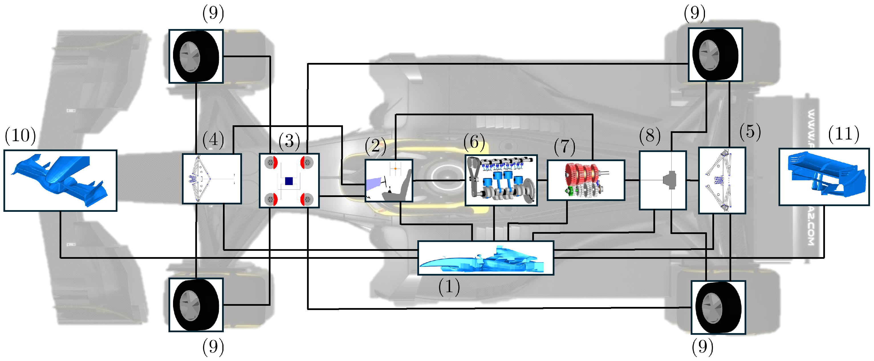
The vehicle model used in this work is a multibody representation integrated within a Driver-in-the-Loop (DiL) simulation environment. The simulated vehicle is a single-seater Formula car manufactured by Dallara (Figure 1), representative of typical modern Formula racing vehicles.

The vehicle model has been developed using the Dymola simulation platform and builds on the VeSyMa Motorsport library [16]. Its overall schematics are depicted in Figure 1. The VeSyMa Motorsport library is specifically designed for the modeling of high-fidelity race cars within simulation environments, with a particular focus on real-time applications such as DiL simulators.

The model features 63 dynamic states and is driven by four inputs: throttle, brake, steering and gear selection. Gear shifts are managed by an engine speed-based control logic that automatically selects gear ratios depending on the current engine RPM, emulating a semi-automatic transmission behavior.

This vehicle model is part of the standard development and validation workflow in Dallara’s DiL simulator, ensuring its fidelity and practical relevance for motorsport applications. The model’s high-fidelity representation is essential for the controller tuning process, as it captures the complex interactions between subsystems that dominate vehicle behavior at the limits of handling.

From a control and optimization perspective, several subsystems are particularly influential for the controller’s inputs and outputs. The tire dynamics are modeled using the Magic Formula formulation [17], capturing nonlinear force-slip relationships and combined slip effects that are critical for accurate lateral and longitudinal force prediction. The tire model directly affects the controller’s ability to track reference trajectories, especially during aggressive cornering and braking maneuvers where tire saturation occurs. The suspension system, implemented as a double wishbone suspension including an anti-roll system, influences vehicle attitude, affecting tire contact forces and thus the effective grip available to the controller. Aerodynamic forces from the front and rear wings are modeled through aerodynamic maps obtained through CFD simulations and wind tunnel tests. These forces generate significant downforce at high speeds, modifying the vertical tire loads and consequently the available lateral and longitudinal forces, which are particularly relevant for the controller’s performance in high-speed sections of the track. Finally, the actuator dynamics (steering, braking, and throttle systems) introduce response delays and limitations that the controller must account for when generating control commands.

Additionally, the model includes a Drag Reduction System (DRS), which can be activated in designated track zones. Its activation is modeled as a variation of the rear wing aerodynamic coefficients, with a reduction in both the lift coefficient ($C_z$) and the drag coefficient ($C_x$), reproducing the real-world mechanism used to decrease drag and increase top speed.

3. Controller Architecture

The vehicle is controlled by a three-loop feedback architecture, with each loop dedicated to a specific actuator: a proportional-derivative (PD) controller for steering, a proportional (P) controller for braking, and a proportional-integral (PI) controller for throttle. These controllers operate in concert to deliver stable, responsive behavior. The selection of this particular controller structure is not arbitrary; it reflects Dallara’s engineering practice, distilled from years of development and application on comparable systems, and is motivated by the physical characteristics and operational requirements of each control loop. Specifically, steering requires damping to prevent oscillations, braking needs a sharp and immediate response, and throttle control employs proportional action for prompt response to speed deviations and integral action to maintain control effort even when the vehicle temporarily exceeds the reference speed.

The optimization process focuses on tuning five specific controller gains: $k_P^{\mathrm{steer}}$, $k_D^{\mathrm{steer}}$, $k_P^{\mathrm{brake}}$, $k_P^{\mathrm{thr}}$, and $k_I^{\mathrm{thr}}$. The role of each gain is discussed in the following subsections of this section. This restricted parameter set is chosen to avoid identifiability issues and redundancy, ensuring a well-posed optimization problem. Several additional coefficients in the control law appear only as multiplicative factors with other terms, and including them as independent decision variables would lead to an over-parameterized problem with redundant solutions.

Each controller combines classical feedback with a preview strategy. The preview term looks ahead along the reference trajectory to anticipate upcoming demands, enabling smoother and more accurate control actions. The preview distance is adjusted online as a function of vehicle speed, allowing the controllers to adapt their responsiveness in both the longitudinal and lateral domains. Separate preview horizons are used for longitudinal control (throttle and brake) and for lateral control (steering), optimizing performance for each subsystem.

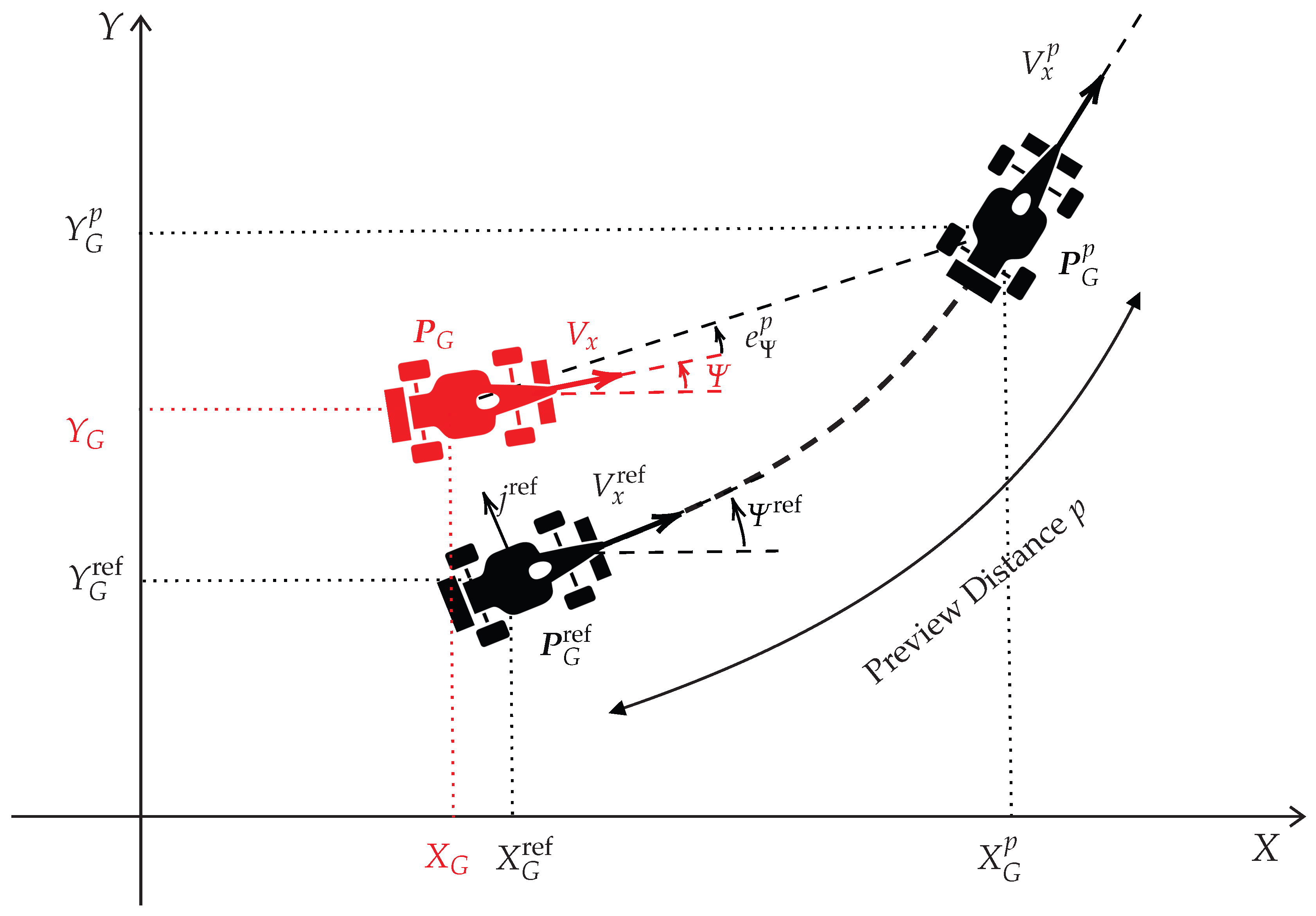
As illustrated in Figure 2, the control strategy relies on the computation of various tracking errors relative to the reference trajectory. Each controller processes these errors to generate the appropriate control signal. Specifically, the current lateral error e represents the instantaneous positional deviation of the vehicle from the reference trajectory, measured in the direction perpendicular to the reference’s forward motion. It is computed as

$$e={\left({\mathbf{P}}_G^{\mathrm{ref}}-{\mathbf{P}}_G\right)}^T{\mathit{j}}^{\mathrm{ref}},$$

(1)

where ${\mathbf{P}}_G^{\mathrm{ref}}$ is the position vector of the reference vehicle, ${\mathbf{P}}_G$ is the position vector of the actual vehicle, and ${\mathit{j}}^{\mathrm{ref}}$ denotes the unit vector normal to the reference trajectory at the current position. Bold symbols are retained to denote vector quantities.

The preview heading error $e_{\Psi }^p$ is defined as the angle between the longitudinal axis of the controlled vehicle and the line from its center of mass to that of the reference vehicle, evaluated at the preview distance (i.e., the origin of the local reference frame at the preview point), as illustrated in Figure 2. This geometric interpretation allows the controller to anticipate heading deviations relative to the future reference trajectory.

The current speed error $e_v$ captures the real-time difference between the vehicle’s longitudinal speed and the reference speed at the current position:

$$e_v=V_x^{\mathrm{ref}}-V_x.$$

(2)

Finally, the preview speed error $e_v^p$ represents the longitudinal speed discrepancy between the vehicle’s current speed and the reference speed at the preview distance. This anticipatory term helps regulate acceleration and braking actions and is given by

$$e_v^p=V_x^p-V_x.$$

(3)

Future tracking errors are obtained by evaluating the reference trajectory at a look-ahead distance, referred to as the preview distance (p). This distance defines a point ahead along the reference path and enables the controller to anticipate forthcoming trajectory states. The preview distance is adaptively scaled with the vehicle’s longitudinal velocity, resulting in longer preview horizons at higher speeds. This adaptive mechanism enhances the controller’s anticipatory behavior, contributing to smoother and more stable responses, particularly during high-speed or highly dynamic maneuvers.

To define the preview distance p, it is convenient to consider the piecewise function defined in (4). This function introduces a saturation behavior between two thresholds, $x_{\mathrm{Thr}}$ and $x_{\mathrm{Lim}}$. For values of x below the lower threshold, the output is kept constant at $y_{\mathrm{Thr}}$, while for values above the upper threshold, it saturates at $y_{\mathrm{Lim}}$. Between these two limits, the function varies linearly, ensuring a smooth transition between the two constant regions.

$$f(x;y_{\mathrm{Thr}},y_{\mathrm{Lim}},x_{\mathrm{Thr}},x_{\mathrm{Lim}})=\left\{\begin{array}{cc}{y}_{\mathrm{Thr}},\hfill & x<x_{\mathrm{Thr}}\hfill \\ y_{\mathrm{Thr}}+{\displaystyle \frac{y_{\mathrm{Lim}}-y_{\mathrm{Thr}}}{x_{\mathrm{Lim}}-x_{\mathrm{Thr}}}}(x-x_{\mathrm{Thr}}),\hfill & x_{\mathrm{Thr}}\le x\le x_{\mathrm{Lim}}\hfill \\ y_{\mathrm{Lim}},\hfill & x>x_{\mathrm{Lim}}\hfill \end{array}\right.$$

(4)

Two distinct preview distances are employed: one for lateral control (steering) and one for longitudinal control (throttle and braking). This distinction reflects the different dynamic requirements of the two subsystems. Specifically, the lateral preview distance is defined as $p=f(V_x;0.4,1,30,75)$, while the longitudinal preview distance is given by $p=f(V_x;0.1,0.7,30,75)$. It is worth noting that the parameters $y_{\mathrm{Thr}}$ and $y_{\mathrm{Lim}}$ are normalized with respect to the maximum value, which corresponds to the longitudinal upper limit $y_{\mathrm{Lim}}$, in order to preserve data confidentiality.

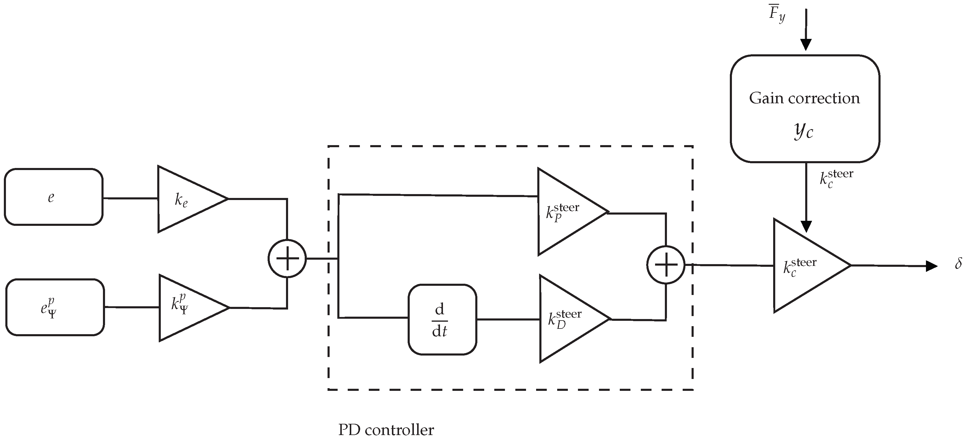
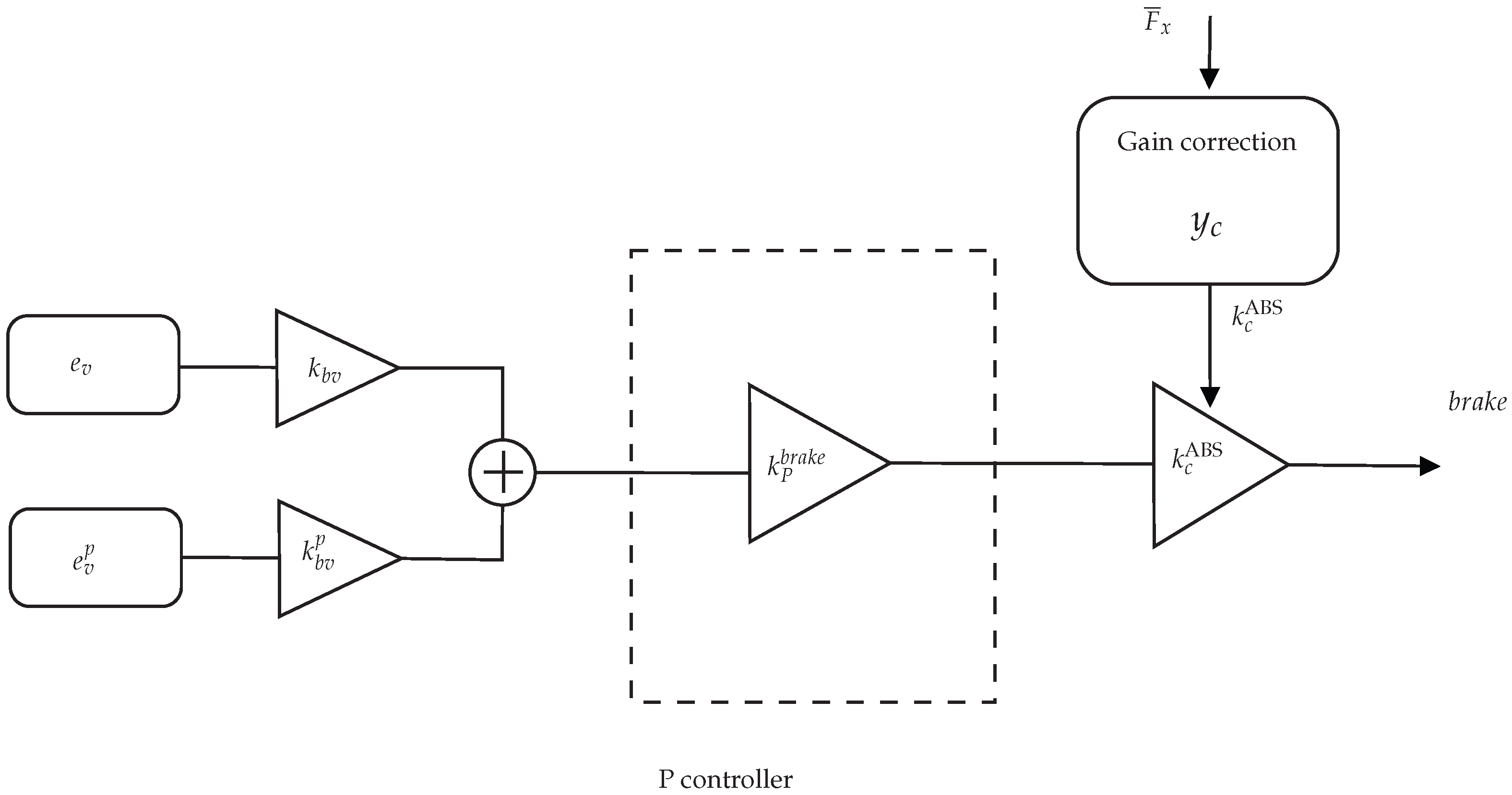
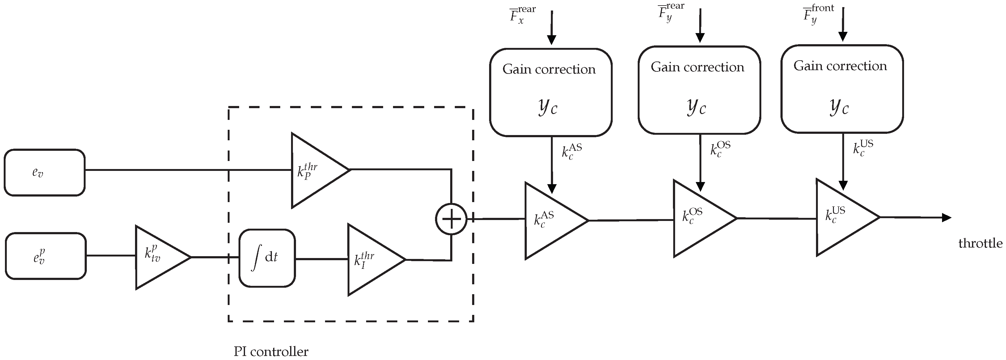
The following sections present schematic representations of the control architectures for steering, throttle, and braking. Although these simplified diagrams do not convey the full implementation details, which are kept confidential due to company policy, they highlight the essential structure and the key tuning parameters employed to optimize controller performance.

3.1. Steering Controller

The controller that generates the steering command ($\delta$) is a Proportional-Derivative (PD) controller that computes the output based on a weighted combination of the current lateral error (e) and the preview heading error ($e_{\Psi }^p$). The PD structure is chosen because steering dynamics require both proportional response to lateral tracking errors and derivative action to provide damping, preventing oscillatory behavior during cornering maneuvers. Figure 3 presents a simplified block diagram of the controller, including the gain parameters that shape its dynamic response.

Downstream of the PD controller, the steering angle command is adjusted based on the level of lateral tire force saturation. The multiplicative correction gain ($y_c$) is computed through the piecewise correction function defined in Equation (4), expressed in its general form as $y_c=f(x;1,0,\mathrm{Thr},\mathrm{Lim})$. The subscript c indicates that the quantity refers to a (multiplicative) correction applied to the nominal control gain. The function takes as input a variable x representing the degree of tire saturation, along with two parameters: a threshold value Thr and a limit value Lim.

This function defines a smooth transition in the applied gain: it outputs the full nominal gain (equal to one) when the tire saturation level is below the threshold value (Thr), then decreases linearly as saturation increases, and finally reaches zero once the saturation exceeds the limit value (Lim), thereby effectively suppressing the control action. In what follows, several correction strategies will be presented; however, the specific values of Thr and Lim are not reported here for confidentiality reasons.

This correction mechanism is applied consistently across all control actions (steering, throttle, and braking) to ensure that commands are attenuated or completely suppressed when tire saturation becomes critical. Such an approach helps prevent excessive slip or instability and maintains control actions within the physical capabilities of the tires, ultimately improving overall vehicle safety and performance.

In the case of the steering controller, the correction is applied through a gain referred to as $k_c^{\mathrm{steer}}=y_c({\overline{F}}_y;1,0,{\mathrm{Thr}}^s,{\mathrm{Lim}}^s)$, which is computed based on the level of lateral tire force saturation ${\overline{F}}_y$ defined as:

$${\overline{F}}_y={\displaystyle \frac{F_y}{\left(D_y-sgn\left(\alpha \right)S{V}_y\right)G_{yk}-S{V}_{yk}sgn\left(\alpha \right)}}$$

(5)

where $\alpha$ denotes the lateral slip angle of the wheel, and $D_y$, $S{V}_y$, $G_{yk}$, and $S{V}_{yk}$ are parameters of the lateral Magic Formula model [17], which serves as the underlying formulation for the tire dynamics implemented in this study. The tire model is parameterized using data from a .tir file corresponding to tires specifically developed for the Dallara Formula car considered in this work. The exact parameter values are not disclosed due to confidentiality constraints.

When the saturation value of any tire exceeds the defined threshold, the correction mechanism is activated and progressively reduces the steering command. This strategy ensures that corrective actions are applied precisely as the tires approach their lateral grip limits, thereby mitigating performance degradation associated with excessive slip angles.

3.2. Brake Controller

The braking controller is implemented as a purely Proportional (P) controller, as the brake signal is intended to be sharp and immediate. The controller structure, illustrated in Figure 4, processes both the current and the preview longitudinal speed errors to compute the braking demand.

As with the steering controller, the braking controller also includes a correction factor based on the saturation of the tire forces, specifically in the longitudinal direction. This correction is applied through a gain called $k_c^{\mathrm{ABS}}$, which is defined as $k_c^{\mathrm{ABS}}=y_c({\overline{F}}_x;1,0,{\mathrm{Thr}}^{\mathrm{ABS}},{\mathrm{Lim}}^{\mathrm{ABS}})$, where $y_c$ is the correction function introduced in (4), and ${\overline{F}}_x$ represents the degree of longitudinal tire saturation. It is explicitly defined as:

$${\overline{F}}_x={\displaystyle \frac{F_x}{\left(D_{x}sgn\left(F_x\right)+S{V}_x\right)G_{x\alpha }}}$$

(6)

where $D_x$, $S{V}_x$, and $G_{x\alpha }$ are parameters of the longitudinal Magic Formula force model [17].

When the value of ${\overline{F}}_x$ exceeds the specified threshold, for at least one tire, the braking command is proportionally reduced. This mechanism, inspired by anti-lock braking system (ABS) logic, helps to prevent wheel lockup during braking phases and ensures safer and more stable vehicle behavior under high deceleration.

3.3. Throttle Controller

The throttle controller, illustrated in Figure 5, is implemented as a Proportional-Integral (PI) controller that processes both current and preview longitudinal speed errors. The proportional component provides a prompt response to speed deviations, enabling quick acceleration when necessary. The integral component, in contrast, maintains a sustained control effort even when the instantaneous speed error $e_v<0$ (i.e., when the vehicle is temporarily faster than the reference). Without this integral action, the control input would drop to zero and could result in a delayed or insufficient throttle response until the error changes sign.

Analogously to the steering and braking loops, the throttle controller employs saturation-based attenuation gains to adapt the commanded drive input under limiting tire conditions. Three complementary correction mechanisms are used, each driven by a specific tire-saturation indicator $\overline{F}$ (normalized utilization, with unity denoting the nominal limit; cf. Equation (4)).

Anti-spin (rear longitudinal). The gain $k_c^{\mathrm{AS}}$ is defined as

$$k_c^{\mathrm{AS}}=y_c\left({\overline{F}}_x^{\mathrm{rear}};1,0,{\mathrm{Thr}}^{\mathrm{AS}},{\mathrm{Lim}}^{\mathrm{AS}}\right),$$

(7)

where ${\overline{F}}_x^{\mathrm{rear}}$ is the rear-axle longitudinal saturation index. This correction mitigates incipient wheelspin by progressively attenuating the throttle as the rear longitudinal utilization approaches and exceeds the limit.

Oversteer mitigation (rear lateral). The gain $k_c^{\mathrm{OS}}$ is defined as

$$k_c^{\mathrm{OS}}=y_c\left({\overline{F}}_y^{\mathrm{rear}};1,0,{\mathrm{Thr}}^{\mathrm{OS}},{\mathrm{Lim}}^{\mathrm{OS}}\right),$$

(8)

based on the rear-axle lateral saturation index. The throttle command is reduced when rear lateral utilization is high, promoting yaw stability and limiting power-oversteer tendencies.

Understeer mitigation (front lateral). The gain $k_c^{\mathrm{US}}$ is defined as

$$k_c^{\mathrm{US}}=y_c\left({\overline{F}}_y^{\mathrm{front}};1,0,{\mathrm{Thr}}^{\mathrm{US}},{\mathrm{Lim}}^{\mathrm{US}}\right),$$

(9)

driven by the front-axle lateral saturation index. By attenuating the throttle under front saturation, the mechanism eases combined-slip demands and induces a mild forward load transfer, thereby improving front-axle cornering authority.

Each correction gain $k_c\in [0,1]$ acts as a scalar attenuation of the nominal throttle command; collectively, these mechanisms enable the controller to maintain stability during traction-limited operation by limiting drive input under critical tire-load conditions.

4. Data Acquisition at Dallara’s Driver-in-the-Loop Simulator

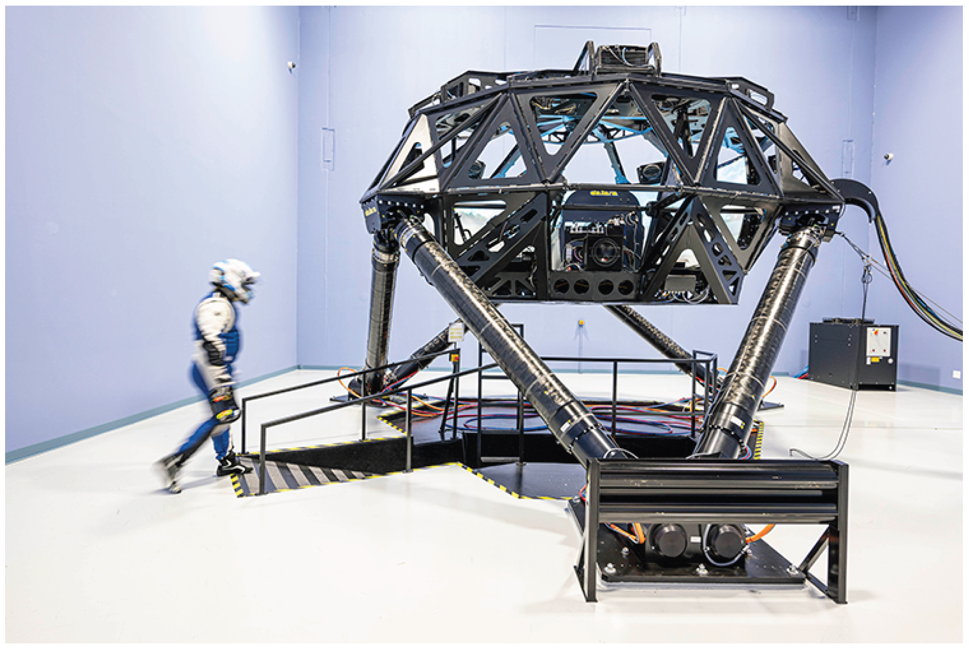
The reference data used by the controller, as well as the data employed for its tuning, were obtained from the company’s Driver-in-the-Loop (DiL) simulator (Figure 6). The simulations within the DiL simulator were performed at a frequency of 1000 Hz, but the output signals were sampled at 100 Hz.

Multiple laps were recorded during the data acquisition session, with the professional driver performing several complete circuits of the Silverstone track. From these recorded laps, a single representative lap was selected as the reference trajectory based on achieving the best balance between lap-time performance and trajectory repeatability, ensuring that the selected lap represents a stable and reproducible driving pattern rather than an outlier with exceptional but non-repeatable performance.

The raw signals from the DiL simulator underwent minimal preprocessing. No explicit filtering was applied, as the simulator’s real-time processing already provides clean, synchronized signals. The data were simply resampled from the internal 1000 Hz simulation frequency to 100 Hz for storage and processing efficiency. The reference trajectory is parameterized as a function of the distance traveled by the vehicle, with position, velocity, and control inputs defined along this spatial coordinate. This parameterization enables the controller to access reference states at any point along the trajectory, supporting the preview strategy employed in the control architecture.

The Dallara DiL is a professional-grade system designed for development and performance engineering. It features a full racing cockpit (monocoque, pedals, steering and braking systems) with high-fidelity force feedback; a multi-channel, high-resolution projection system with a high refresh rate; and a real-time software stack for deterministic, closed-loop operation. The visual system employs dome-calibrated, multi-projector rendering with automated geometric and photometric alignment to ensure seamless imagery across the dome. The overall architecture allows engineers to configure the vehicle model, track environment and controller parameters and log-synchronized channels for both driver inputs and vehicle states.

In the present study, the controller and vehicle model run against the simulator’s real-time clock. Driver commands (throttle, brake, steering and gear selection) are acquired with low-latency interfaces and fed to the vehicle model; the resulting torques, forces and states are returned to the haptic and visualization subsystems within the same real-time cycle. End-to-end timing is engineered to preserve driver controllability at high vehicle dynamics bandwidths. All signals used for reference trajectory generation and controller calibration are time-stamped and synchronized with the simulator clock.

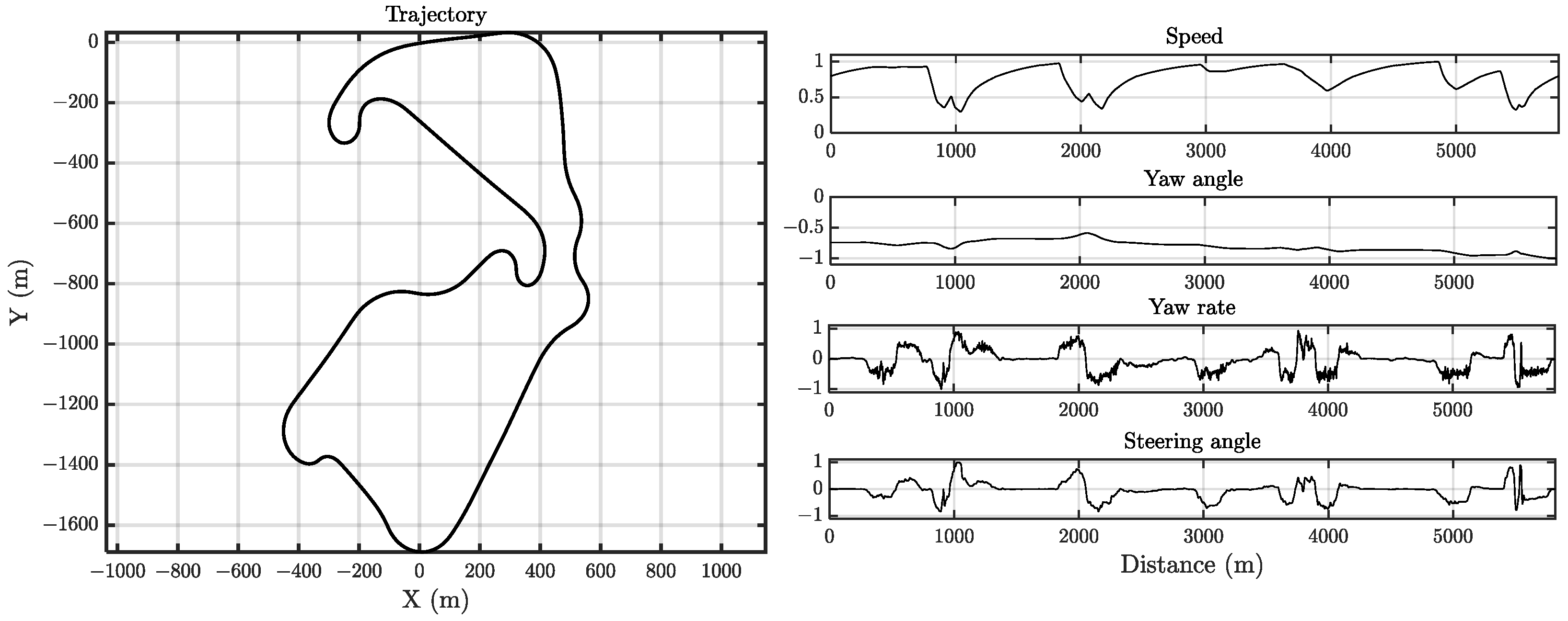
Figure 7 shows the datasets used both for reference trajectory generation and for controller calibration. Due to confidentiality agreements with the company, the data have been normalized.

The professional driver completed the simulator lap in $t_{\mathrm{end}}^{\mathrm{ref}}$ = 99.19 s. This lap time is used as the simulation horizon within the optimization framework, which will be detailed in the next section.

It is important to note that the objective of this study is not to generalize across multiple drivers or circuits, but rather to faithfully reproduce a specific, expert reference performance in a well-defined high-performance scenario. The methodology is tailored to the particular combination of vehicle model, track layout, and professional driver reference data analyzed here. Generalization to other contexts, such as different circuits, drivers, or vehicle configurations, represents an important direction for future research but is beyond the scope of the present work.

5. Optimization-Based Tuning Framework

This section outlines the optimization framework employed for tuning the controller parameters with the objective of minimizing lap time. The optimization process focuses on adjusting the gains of the controllers described in the previous sections. These gains serve as the decision variables within the optimization routine. Specifically, the optimization variable vector is defined as

$$\mathit{k}=[k_P^{\mathrm{steer}},k_D^{\mathrm{steer}},k_P^{\mathrm{brake}},k_P^{\mathrm{thr}},k_I^{\mathrm{thr}}].$$

(10)

We restrict the optimization to the gains in $\mathit{k}$ because several additional coefficients introduced in Section 3 enter the control law only as multiplicative factors with other terms. Including such coefficients as independent decision variables would lead to an over-parameterized problem with redundant solutions, since the closed-loop effect depends on their product rather than on the individual factors.

For instance, if two coefficients $\alpha$ and $\beta$ appear in the controller as a product $\alpha \beta g(·)$, then any rescaling $\alpha \leftarrow \gamma \alpha$, $\beta \leftarrow \beta /\gamma$ with $\gamma >0$ leaves the product $\alpha \beta$ (and therefore the closed-loop behavior) unchanged. Optimizing both $\alpha$ and $\beta$ would thus introduce non-identifiability (flat directions in the cost landscape) and unnecessary ill-conditioning. By fixing such auxiliary scalings to their nominal values and optimizing only the core gains $\mathit{k}$, we preserve the full achievable performance while improving numerical conditioning and interpretability of the solution.

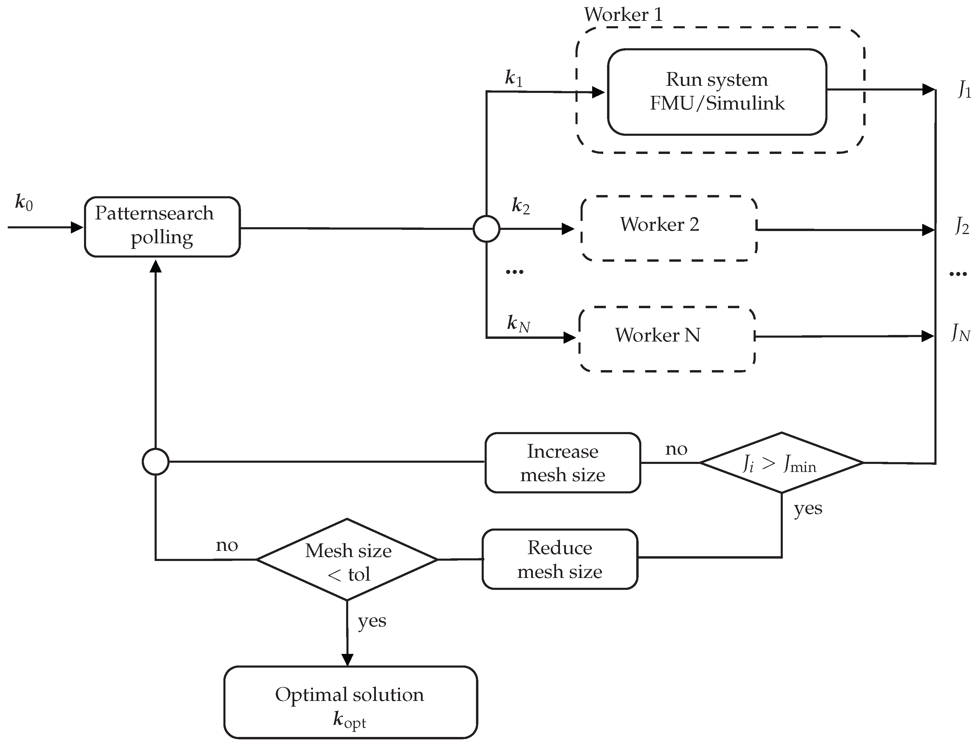
The optimization process (as illustrated in Figure 8) employs the PatternSearch algorithm [18], as implemented in MATLAB’s Global Optimization Toolbox. This is a derivative-free optimization method [19], making it particularly suitable for our application. In fact, the combined Vehicle + Controller system is exported from Dymola as an FMU 2.0 (Functional Mock-up Unit) [20] and integrated into a Simulink environment. As a result, the system behaves as a black-box model, where internal dynamics are not directly accessible. The optimizer can therefore only modify the controller gain values and observe the resulting outputs, which are used to evaluate an appropriately defined cost function.

Starting from an initial set of controller gains ${\mathit{k}}_0$, the optimization begins with a polling phase, during which multiple candidate sets of ${\mathit{k}}_i$ are generated and distributed across parallel workers. Each worker then runs a separate simulation of the system in Simulink at a sampling frequency of 1000 Hz, and the corresponding value of the cost function $J_i$ is evaluated for each candidate.

The patternsearch algorithm is configured with the following operational parameters to ensure reproducibility. The controller gains are normalized with respect to their maximum values to aid the optimization algorithm. The search bounds for each normalized gain are defined as: $k_P^{\mathrm{steer}}\in [0,5]$, $k_D^{\mathrm{steer}}\in [0,0.05]$, $k_P^{\mathrm{brake}}\in [0,50]$, $k_P^{\mathrm{thr}}\in [0,5]$, and $k_I^{\mathrm{thr}}\in [0,5]$, where the upper bounds correspond to the maximum expected values for each gain. The algorithm employs a Generalized Pattern Search (GPS) exploration strategy with a positive basis of $2N$ directions (PollMethod: ‘GSSPositiveBasis2N’), where $N=5$ is the number of optimization variables. The stopping criteria include: (i) a maximum number of iterations set to ${10}^4$, (ii) a maximum number of function evaluations set to ${10}^4$, (iii) a function tolerance of ${10}^{-4}$ (relative change in objective function value), (iv) a mesh tolerance of $0.02$, and (v) a step tolerance of $0.02$. The optimization terminates when any of these criteria is satisfied.

Based on the polling results, the mesh size used for the search is adaptively updated: if a lower cost value is found (a successful poll), the mesh size is increased by a factor of 1.5 (MeshExpansionFactor) to accelerate convergence; otherwise, it is reduced by a factor of 0.7 (MeshContractionFactor) to refine the search. The maximum mesh size is set to 1. This iterative process continues until the stopping criteria of the algorithm are met, yielding the optimal set of controller gains ${\mathit{k}}_{\mathrm{opt}}$.

Preliminary tests investigating the sensitivity of the optimization result to the initial guess ${\mathit{k}}_0$ showed that while different initial conditions can lead to slightly different local optima, the final cost function values and controller performance are consistent across multiple runs, suggesting a well-defined region of good solutions.

During the optimization, certain sets of variables may trigger a simulation failure (e.g., vehicle rollover or numerical instability). Whenever this occurs, we assign a large penalty to the objective (specifically, set the cost to ${10}^6$). This barrier-like penalization effectively discards infeasible solutions by marking the corresponding region of the parameter space as highly unattractive while preserving the cost function landscape for valid solutions without distorting the relative ordering of feasible parameter sets. This approach is particularly important for derivative-free methods like patternsearch, which rely on the relative ordering of function values to navigate the search space effectively.

5.1. Cost Function Structure

This section presents the cost function that underpins our simulation-based optimization framework. Because the vehicle model is handled as a black box, performance and constraint evaluation are carried out via time-domain simulations. The primary objective is to reduce lap time; with a fixed simulation horizon, this is pursued by maximizing the distance covered. Constraint compliance is promoted through embedded penalty terms (penalty-function approach [21]), with weights selected to enforce feasibility without overshadowing the main objective. In particular, penalties are imposed on both the state trajectories and the control-input trajectories generated by the controller under optimization, constraining their deviation from the professional driver’s reference.

In this context, “human-likeness” is operationalized through similarity in three specific aspects: (i) path tracking (lateral error), (ii) speed profile (velocity error), and (iii) frequency content of the steering signal. This definition is not intended as a holistic measure of human driving behavior, but rather as a targeted metric to ensure that the optimized controller reproduces key characteristics of the professional driver’s reference performance in these specific domains.

In this way, the optimization injects an explicit human-likeness prior into the discovered controller while preserving the primacy of lap-time performance. Altogether, the formulation yields a single, tunable criterion that balances lap-time performance with robustness and constraint satisfaction.

The cost function used in this work is

$$J=d\left(s\right)+\left[H_{\delta }+d_{\delta }+{\displaystyle \frac{\rho }{N_{T}N}}\sum _{i=1}^N\left(d_{e_i}+d_{v_i}\right)\right].$$

(11)

Here, $d\left(s\right)$ expresses the primary goal of minimizing lap time, while the terms enclosed in square brackets are the penalty terms enforcing human-likeness. The latter terms must vanish or be very small at the solution compared to $d\left(s\right)$ for the constraints to be satisfied in practical terms.

5.1.1. Lap Time

Since the simulation horizon is fixed, maximizing the distance traveled by the controlled vehicle within that horizon is a proxy for minimizing lap time. To enforce this, which is the primary goal, we minimize $d\left(s\right)={\displaystyle \frac{s^{\mathrm{ref}}-s}{\overline{s}}}$, where $s^{\mathrm{ref}}$ is the arc length covered by the reference lap, s is the arc length covered by the controlled vehicle, and $\overline{s}>0$ is a normalization length. In this study, we set $\overline{s}=0.01s^{\mathrm{ref}}$ for numerical scaling. The term $d\left(s\right)$ is monotonically decreasing in s: $d\left(s\right)=1$ when the distance deficit $(s^{\mathrm{ref}}-s)=\overline{s}$ and $d\left(s\right)=0$ when $s=s^{\mathrm{ref}}$. It is positive and grows linearly with the distance deficit $(s^{\mathrm{ref}}-s)$ and becomes negative if $s>s^{\mathrm{ref}}$, thus rewarding trajectories that cover more distance within the same horizon. Because J is minimized, this term drives s upward (i.e., encourages a larger distance within the fixed time window), thereby indirectly favoring shorter lap times.

5.1.2. Lateral Error and Velocity Error Penalty Terms

The terms $d_{e_i}$ are associated with the constraint on the lateral error e with respect to the reference trajectory, while $d_{v_i}$ are associated with the constraint on the velocity error $e_v$ with respect to the reference. N is the number of samples, and $N_T$ is the number of terms included in the summation ($N_T=2$ in our tests). The normalization by $N_{T}N$ makes the contribution essentially independent of the sampling rate and the number of active terms. The coefficient $\rho$ is used as an exact-penalty weight. Choosing $\rho$ sufficiently large ($\rho =100$ in our tests) ensures that, whenever violations occur, the aggregate penalty dominates J and the optimizer is effectively guided to parameter regions where these penalties are satisfied at the solution. This is consistent with the rationale of exact penalty methods.

In more detail, at the i-th sampling instant, the element $d_{e_i}$ is:

$$d_{e_i}=\left\{\begin{array}{cc}0,\hfill & |e_i|\le b_e\hfill \\ {\displaystyle \frac{|e_i|-b_e}{b_e}},\hfill & |e_i|>b_e\hfill \end{array}\right.,$$

(12)

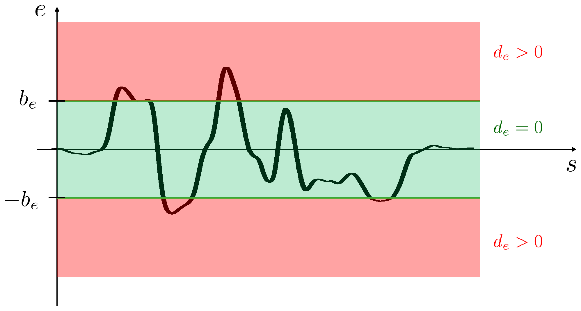
where $b_e$ represents the bound used for the lateral error constraint. $b_e$ is set to 2 m in our tests. By construction, the penalty for the i-th sample activates only when the lateral error exceeds its admissible bound. Specifically, if $|e_i| \le b_e$ then $d_{e_i}=0$; if $|e_i| >b_e$ then $d_{e_i}>0$ and increases with the violation magnitude $|e_i| - b_e$, thereby contributing to the total cost in proportion to the constraint breach. Figure 9 illustrates this dead zone behavior: no penalty within the bound and a growing penalty beyond it.

The second term within the summation $d_{v_i}$ is associated with the constraint on the velocity error with respect to the reference. At each sampling instant, it is defined as:

$$d_{v_i}=\left\{\begin{array}{cc}0,\hfill & e_{v_i}\le b_v\hfill \\ {\displaystyle \frac{e_{v_i}-b_v}{b_v}},\hfill & e_{v_i}>b_v\hfill \end{array}\right.$$

(13)

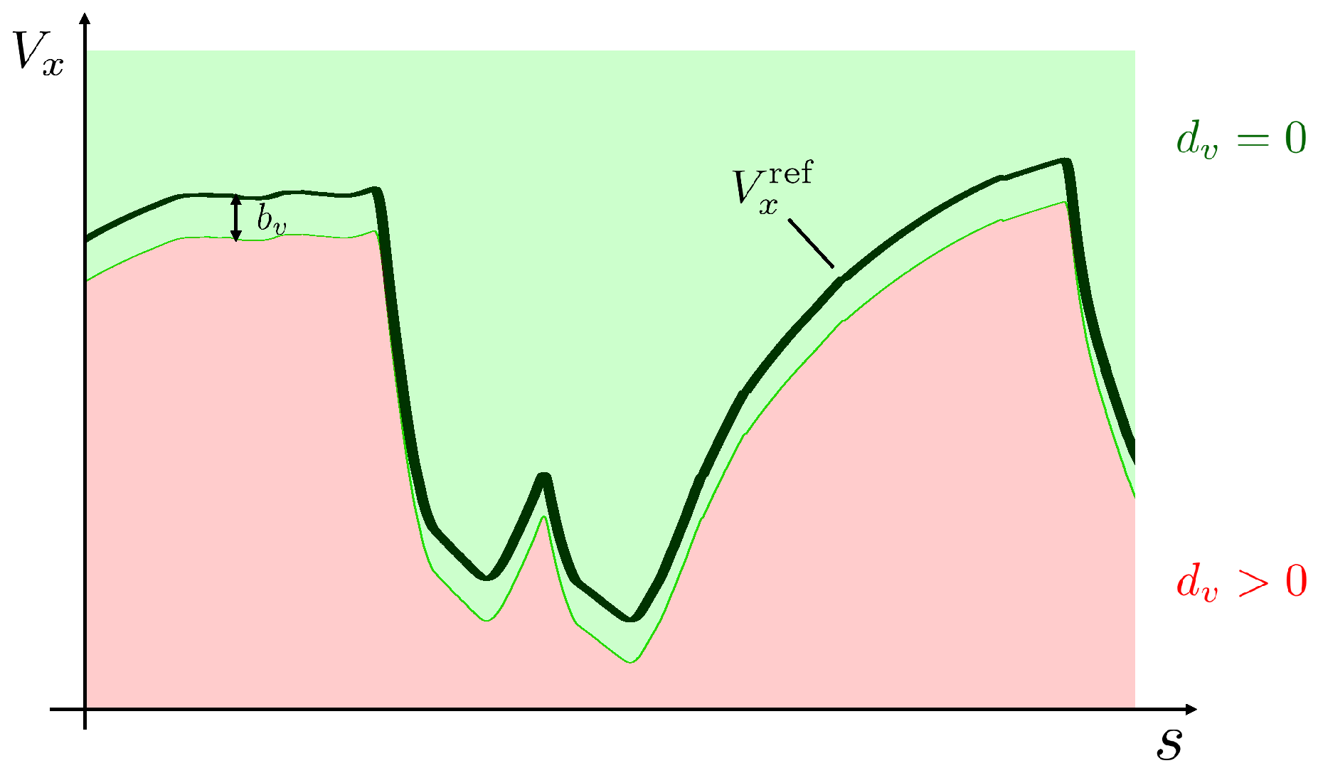
Here, $b_v$ represents the bound for the velocity constraint, which is set to 7 m/s in our tests. Similarly to the lateral error constraint, a penalty is applied to the velocity tracking when the speed deficit exceeds the admissible tolerance. It is worth stressing that this penalty is one-sided: defining the instantaneous velocity error as $e_{v,i}=V_{x,i}^{\mathrm{ref}}-V_{x,i}$, we set $d_{v_i}=0$ for $e_{v,i}\le b_v$ and activate the penalty ($d_{v_i}>0$) only when $e_{v,i}>b_v$, i.e., when the controlled vehicle lags the reference by more than $b_v$. Figure 10 illustrates this one-sided dead zone: no penalty when the vehicle matches or exceeds the reference speed or when the deficit is within tolerance and a growing penalty beyond $b_v$. This setup enables the controller—when permitted by its architecture—to tune parameters that outperform the human driver, who serves here as an improvable reference baseline.

5.1.3. Human-Likeliness Penalties for Steering

The remaining two terms, $H_{\delta }$ and $d_{\delta }$, concern the steering command generated by the controller. The term $H_{\delta }$ enforces a hard bound on the peak steering angle via a barrier-type penalty:

$$H_{\delta }=\left\{\begin{array}{cc}0,\hfill & {\displaystyle \underset{1\le i\le N}{max}\left|{\delta }_i\right|\le {\delta }_{max},}\hfill \\ C_H,\hfill & {\displaystyle \underset{1\le i\le N}{max}\left|{\delta }_i\right|>{\delta }_{max},}\hfill \end{array}\right.$$

(14)

with ${\delta }_{max}=\pi$ rad and $C_H=5$, where ${\delta }_i$ denotes the steering angle at the i-th sample. This construction acts as a barrier: any violation of the amplitude bound incurs a fixed penalty $C_H$, effectively excluding parameter regions that yield unrealistically large steering commands.

The companion term $d_{\delta }$ provides a smooth usage regularization on the steering signal (e.g., penalizing excessive activity/energy or rate), thereby promoting well-conditioned control actions. In more detail, $d_{\delta }$ regularizes the steering angle signal, avoiding high-frequency oscillations and ensuring human-like behavior. To this end, a frequency-domain analysis is performed on both the reference steering signal ${\delta }^{\mathrm{ref}}\left(t\right)$ and the signal generated by the controller $\delta \left(t\right)$.

First, the discrete Fourier transform (DFT) of the signals is computed as

$${\Delta }^{\mathrm{ref}}\left(k\right)=\sum _{n=0}^{N-1}{\delta }^{\mathrm{ref}}\left(n\right)e^{-j2\pi kn/N},\Delta \left(k\right)=\sum _{n=0}^{N-1}\delta \left(n\right)e^{-j2\pi kn/N}$$

(15)

where N is the number of samples. The spectral energy distributions are then obtained as

$$E^{\mathrm{ref}}\left(k\right)={\left|{\Delta }^{\mathrm{ref}}\left(k\right)\right|}^2,E\left(k\right)={\left|\Delta \left(k\right)\right|}^2$$

(16)

and are employed to compute the total energies of the two signals as follows

$$E_{\mathrm{tot}}^{\mathrm{ref}}=\sum _{k=0}^{N/2}{E}^{\mathrm{ref}}\left(k\right),E_{\mathrm{tot}}=\sum _{k=0}^{N/2}E\left(k\right).$$

(17)

Next, the energy content is partitioned into three frequency bins: $f\in [0,1]$ Hz, $f\in [1,2]$ Hz, and $f>2$ Hz. These frequency intervals were determined through preliminary optimization runs without the steering frequency penalty term, which revealed that controllers tended to generate excessive control activity in these frequency ranges, significantly differing from the driver’s reference behavior.

For each bin b, the percentage of energy with respect to the total signal energy is then computed as

$$P^{\mathrm{ref}}\left(b\right)={\displaystyle \frac{{\sum }_{k\in b}{E}^{\mathrm{ref}}\left(k\right)}{E_{\mathrm{tot}}^{\mathrm{ref}}}},P\left(b\right)={\displaystyle \frac{{\sum }_{k\in b}E\left(k\right)}{E_{\mathrm{tot}}}}.$$

(18)

The dissimilarity between the two distributions is quantified using a divergence measure inspired by the Kullback-Leibler divergence [22]. Specifically, we define

$${\mathcal{D}}_{\delta }=\sum _{b}w\left(b\right)\left|log\left({\displaystyle \frac{P\left(b\right)}{P^{\mathrm{ref}}\left(b\right)}}\right)\right|,$$

(19)

where the weights $w\left(b\right)$ are normalized such that ${\sum }_{b}w\left(b\right)=1$ and increase with the bin frequency. In contrast to the classical KL divergence, this formulation (i) uses absolute values to measure discrepancies regardless of their sign, and (ii) introduces the weighting vector $w\left(b\right)$ to place greater emphasis on higher frequency bins. With the classical KL divergence, in fact, it would not be possible to clearly capture differences between the two distributions, since the energy percentage in the first frequency bin is significantly higher than in the others, which would always lead to very small values of ${\mathcal{D}}_{\delta }$. This choice is motivated by the objective of discouraging high-frequency oscillations in the steering signal, which would otherwise result in unrealistic steering oscillations even along straight sections of the track.

For numerical robustness, a small regularization constant $ϵ={10}^{-12}$ is added to both $P\left(b\right)$ and $P^{\mathrm{ref}}\left(b\right)$ before computing the logarithm in the divergence calculation, ensuring numerical stability while preserving the relative ordering of the distributions.

The penalty term $d_{\delta }$ is then defined as

$$d_{\delta }=max\left({\mathcal{D}}_{\delta }-b_{\delta },0\right).$$

(20)

In this way, when ${\mathcal{D}}_{\delta }$ exceeds the threshold $b_{\delta }$, the term contributes to the cost function, while it is equal to zero otherwise. In this work, the choice $b_{\delta }=0.35$, made through empirical testing, guarantees a suitable trade-off between controller performance and realism of the steering signal.

6. Results

In this section, we compare the proposed simulation-based tuning with a manual calibration of the controller gains. While careful manual tuning can yield good results, it is time-consuming and requires substantial expertise and sensitivity to the coupled effects of multiple parameters, making it difficult to consistently balance competing objectives. By contrast, the simulation-based optimization provides a systematic and reproducible procedure: it explores the parameter space coherently and explicitly, enforces human-likeness through penalty terms, and consistently achieves a better trade-off between maximizing distance over the fixed horizon and preserving realistic driving behavior.

The optimization was executed on a high-performance computing cluster provided by the Sistema Informatico Dipartimentale (SID), Università di Pisa, Pisa, Italy, equipped with four Intel^® Xeon^® Platinum 8260L CPUs (2.40 GHz base, up to 3.40 GHz boost) and 3.70 TB of RAM, for a total of 96 CPU cores. For the present workload, the available compute capacity was intentionally oversized: we limited the number of worker processes to $10=2\times N_k$ (with $N_k=5$ controller parameters) to match the intrinsic parallelism of the Patternsearch algorithm and avoid idle resources. The abundant RAM was nevertheless beneficial, as it allowed all simulation data, temporary buffers, and logs to reside in memory, minimizing I/O and eliminating paging. The complete optimization required $8.513\times {10}^3$ s (≈2 h 22 m) of wall-clock time.

Overall, the results highlight the effectiveness of the automated optimization framework in tuning the controller parameters while ensuring a realistic driving style. Compared to manual tuning, the proposed approach offers a structured way to reconcile human-like control behavior with the maximization of the track coverage, thereby producing a more balanced and reliable outcome.

The optimizations start from an initial set of controller parameters that are not able to properly drive the vehicle.

Table 1. Initial controller parameters and values obtained through manual (Manual tuning) and optimization-based tuning (Optimal tuning).

	${\mathit{k}}_{\mathit{P}}^{\mathbf{steer}}$	${\mathit{k}}_{\mathit{D}}^{\mathbf{steer}}$	${\mathit{k}}_{\mathit{P}}^{\mathbf{brake}}$	${\mathit{k}}_{\mathit{P}}^{\mathbf{thr}}$	${\mathit{k}}_{\mathit{I}}^{\mathbf{thr}}$
Start value	0.5	0.003	9	0.8	0.3
Manual tuning	0.65	0.001	40	0.5	0.5
Optimal tuning	1.25	0.003	14	0.8253	0.6375

shows the initial parameters ${\mathit{k}}_0$ together with those obtained through manual tuning and the proposed automated optimization-based tuning.

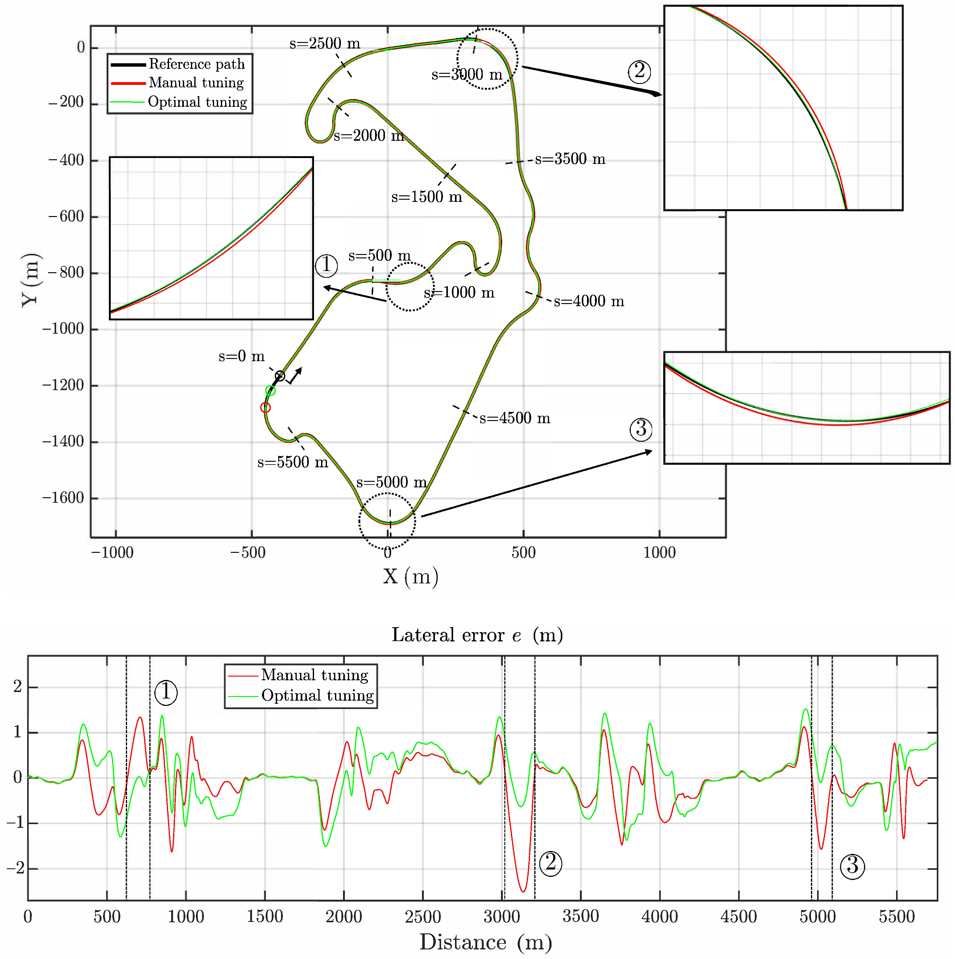
In Figure 11, the trajectories of the reference driver, the vehicle controlled with manually tuned parameters (Manual tuning), and the one controlled with optimization-based tuning (Optimal tuning) are compared.

The figure shows that the vehicle driven by the optimized controller covers a larger distance compared to the manually tuned one. Specifically, the total distance traveled by the reference driver is $s^{\mathrm{ref}}=5820.1$ m, while the vehicle with manual tuning covers $s^{\mathrm{man}}=5693.3$ m and the one with optimization-based tuning reaches $s^{\mathrm{opt}}=5756.9$ m, corresponding to an improvement of $63.6$ m (1.1% increase in distance covered) with respect to the manually tuned case.

Figure 11 shows the evolution of the lateral error e, defined in Equation (1). Highlighted regions (➀, ➁ and ➂) correspond to sections of the track where the lateral errors of the manually tuned and optimized controllers differ significantly. These regions are characterized by combined slip conditions, where the tires simultaneously experience both lateral forces (due to steering) and longitudinal forces (due to throttle application). Under combined slip, the available tire force is shared between lateral and longitudinal directions, creating a coupled interaction between the steering and throttle control loops. The optimized controller handles these conditions better than manual tuning by simultaneously coordinating all gains to find a globally balanced solution, whereas manual tuning, which typically adjusts gains sequentially, struggles to capture these coupled interactions effectively.

In particular, in region ➁ the condition $\left|e\right|>b_e=2$ m is violated in the manually tuned case, thus triggering the penalty term $d_e$ introduced in the cost function and defined in Equation (12).

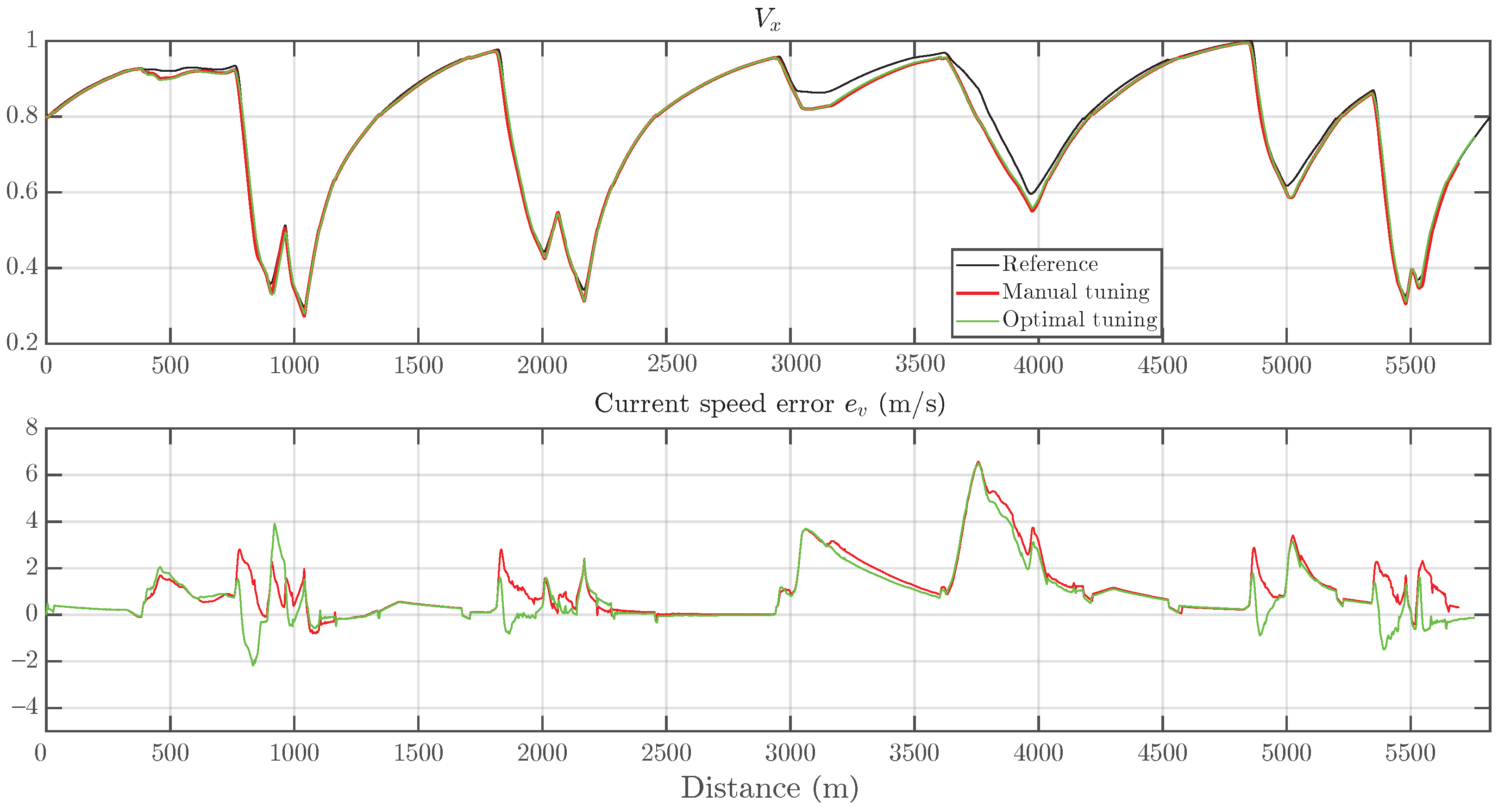
In Figure 12, the longitudinal velocity profiles of the three vehicles are compared. For confidentiality reasons, the velocities are normalized with respect to the maximum velocity of the reference driver.

Both the manually tuned and optimization-based controllers closely follow the reference velocity profile, except for certain sections of the track. These deviations are primarily due to inherent limitations of the controllers, which cannot fully capture the behavior of a human driver, especially in regions where the tires experience excessive combined slip. In such demanding sections, the human driver’s ability to adaptively modulate control inputs based on tactile feedback and experience provides advantages that the fixed-architecture controller cannot fully replicate. The optimized controller, however, achieves a better balance by systematically tuning the gains to better handle combined slip conditions, resulting in improved lateral error control in these challenging regions, as discussed earlier in relation to the highlighted track sections.

Figure 12 also reports the evolution of the current speed error $e_v$, defined in Equation (3). In some areas, the error becomes negative ($e_v<0$), particularly during braking zones where the optimization-based controller applies braking slightly later than the reference. This indicates that, in these sections, the controlled vehicle is moving faster than the reference driver as allowed by the structure of penalty terms $d_{v_i}$ in Equation (13).

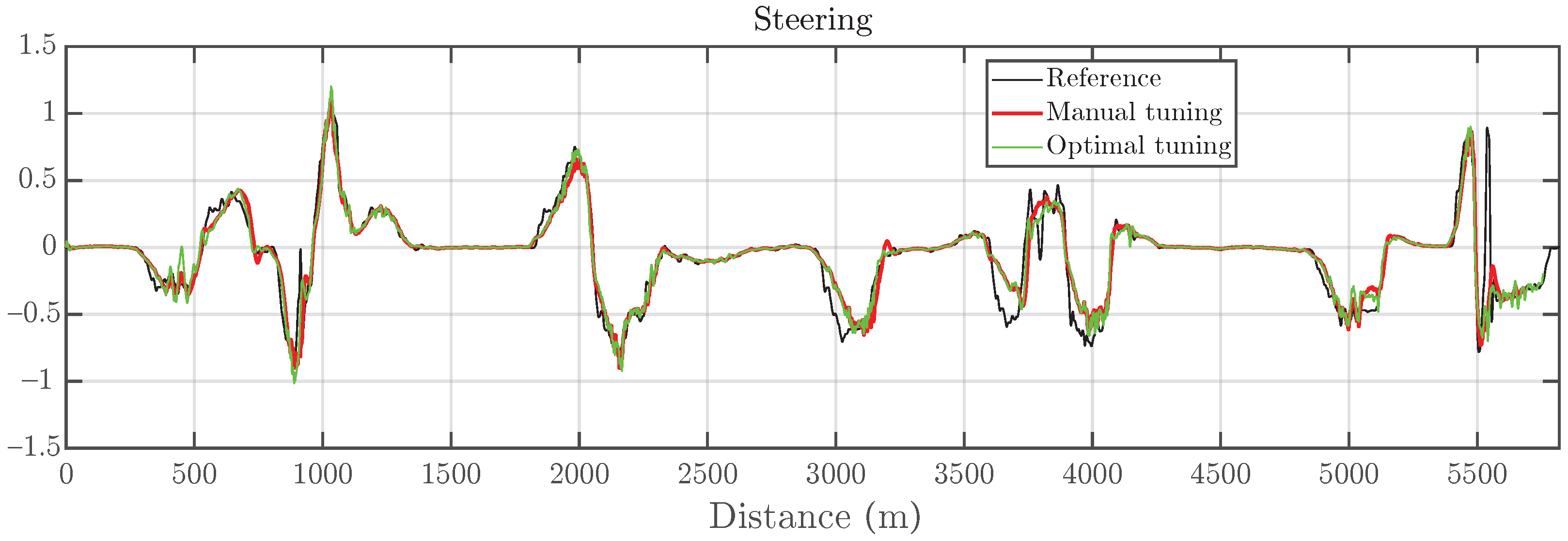
In Figure 13, the steering angle signals for the three cases are compared.

Both the manually tuned and optimization-based controllers reproduce the reference driver’s steering behavior, except for certain regions characterized by high combined tire slip, where deviations become more pronounced.

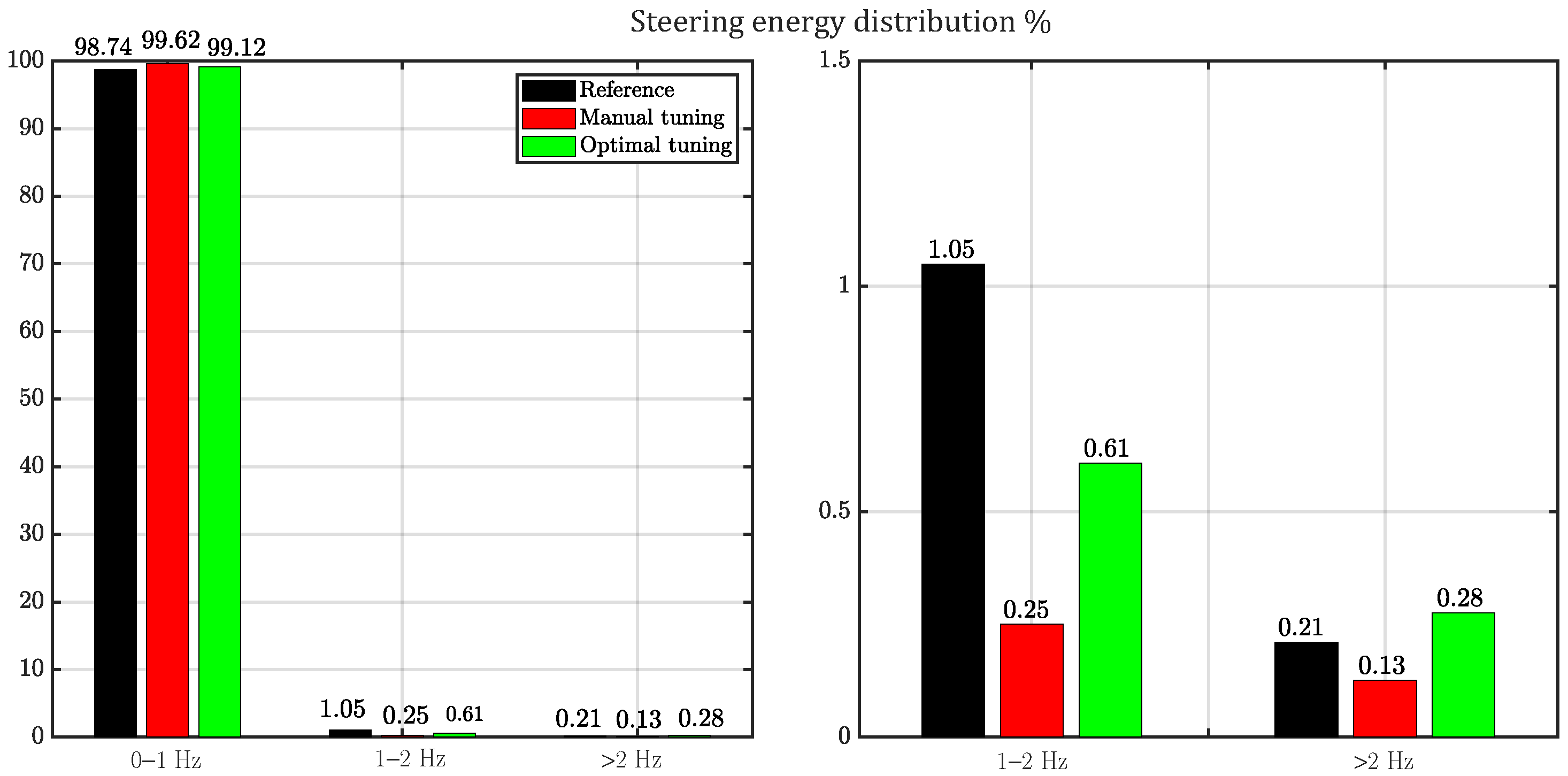
It is also interesting to analyze the energy distribution of the steering signal across the different frequency bins, as defined in Section 5.1. This is shown in Figure 14.

The differences between the reference and the controlled signals are smaller in the optimization-based tuning case. This behavior is due to the presence of the penalty term $d_{\delta }$, defined in (20), within the cost function, which drives the optimization to minimize such discrepancies. In contrast, for the manual tuning case, a residual contribution of this term remains.

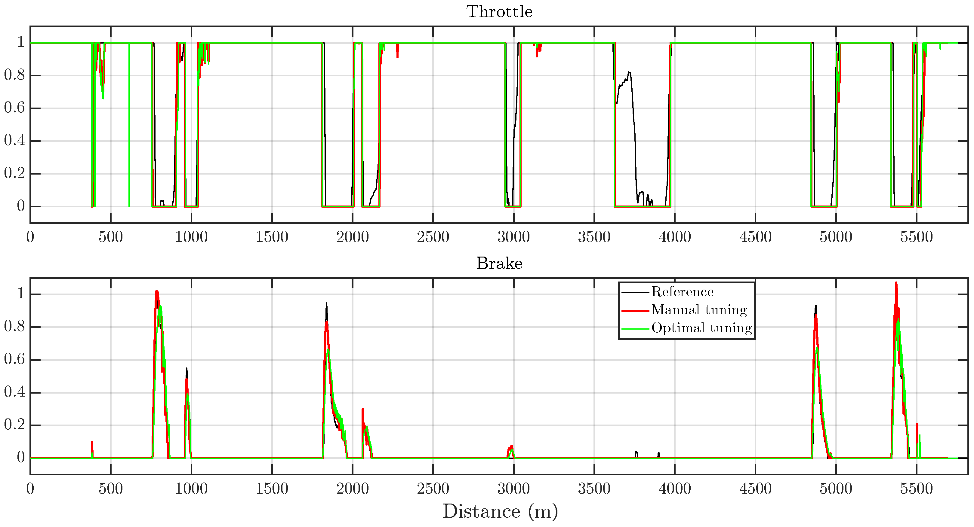
For completeness, Figure 15 shows the comparison of the remaining control inputs: throttle and brake.

As can be seen, the throttle control signals are very similar for both tuning approaches. However, due to intrinsic controller limitations, neither of them is able to accurately follow the reference in sections where partial throttle modulation occurs. Regarding the brake control, the optimization-based controller tends to apply braking slightly later and with lower intensity compared to the other cases. This behavior is consistent with the observations discussed earlier, where the current speed error $e_v$ becomes negative in these same regions.

Table 2. Breakdown of cost-function terms at the solutions for manual tuning (Manual Tuning) and optimization-based tuning (Optimal tuning).

	$\mathit{d}\left(\mathit{s}\right)$	${\mathit{H}}_{\mathit{\delta }}$	${\mathit{d}}_{\mathit{\delta }}$	$\frac{\mathit{\rho }}{{\mathit{N}}_{\mathit{T}}\mathit{N}}{\sum }_{\mathit{i}=1}^{\mathit{N}}{\mathit{d}}_{{\mathit{e}}_{\mathit{i}}}$	$\frac{\mathit{\rho }}{{\mathit{N}}_{\mathit{T}}\mathit{N}}{\sum }_{\mathit{i}=1}^{\mathit{N}}{\mathit{d}}_{{\mathit{v}}_{\mathit{i}}}$
Manual Tuning	2.1779	0	0.3367	0.1039	0
Optimal tuning	1.0850	0	0	0	0

reports a breakdown of the terms in the cost function for the two calibration strategies, Manual Tuning and Optimal Tuning, at their solutions.

In Optimal Tuning, all penalty terms vanish ($H_{\delta }=0$, $d_{\delta }=0$, $d_e=0$, $d_v=0$), leaving $d\left(s\right)$ as the only nonzero contribution to the objective. This outcome is fully consistent with the exact-penalty design: at the solution, constraint violations are driven to zero, and the cost reduces to the primary objective. Moreover, $d\left(s\right)$ is lower than in Manual Tuning (1.0850 vs. 2.1779), indicating that the optimized controller covers a longer distance over the fixed horizon, i.e., yields a more efficient trajectory.

In Manual Tuning, heuristic trial-and-error adjustments appear to have targeted specific constraints—$d_v=0$ (no velocity-deficit penalty) and $H_{\delta }=0$ (peak steering within bounds). However, two penalties remain active: the lateral-error term $d_e=0.1039$, consistent with the observed peaks beyond tolerance (cf. Figure 11), and the steering dissimilarity term $d_{\delta }=0.3367$, reflecting a distributional divergence ${\mathcal{D}}_{\delta }$ (cf. Equation (19)) above the threshold. This suggests that, while the manual process can satisfy selected constraints, it struggles to jointly enforce all requirements and to balance them against the distance objective in a consistent manner.

Finally, we note that an objective breakdown of which penalties are active can aid a human tuner; nonetheless, managing the coupled effect of multiple parameters with a manual, heuristic approach is practically unfeasible within a reasonable time, whereas the optimization systematically enforces the penalties and prioritizes the primary objective by construction.

7. Discussion

The results demonstrate the effectiveness of the automated optimization framework in tuning the controller parameters while ensuring a realistic driving style. The key advantage of outperforming manual tuning lies in the optimization’s ability to capture the coupled nature of the control loops more effectively than sequential manual calibration. As discussed in Section 6, the most demanding track sections are characterized by combined slip conditions, where steering and throttle control loops interact strongly. The optimization simultaneously tunes all gains, finding a globally balanced solution that accounts for these coupled interactions, whereas manual tuning typically adjusts gains sequentially or independently, missing the optimal coordination. This systematic approach enables the optimization to jointly enforce all constraints (lateral error bounds, speed deficits, steering frequency content) while maximizing distance coverage, resulting in a more balanced trade-off between performance and human-likeness.

The optimization systematically enforces all penalty terms and prioritizes the primary objective by construction, eliminating the need for time-consuming manual trial-and-error adjustments that are sensitive to parameter coupling. As shown in Table 2, while manual tuning can satisfy selected constraints, it struggles to jointly enforce all requirements, leaving residual penalties that the optimization successfully eliminates.

It is important to acknowledge the limitations of this study. The results are specific to a single circuit, a single professional driver’s reference data, and a fixed controller architecture. The lack of cross-validation on other tracks or with other drivers means that the generalizability of the optimized gains to different contexts remains an open question. Future work should investigate the transferability of the tuning procedure across different tracks, drivers, and potentially different vehicle configurations, as well as explore the sensitivity of the results to variations in track conditions and reference driving styles.

8. Conclusions

The proposed simulation-based procedure automatically tunes a predetermined triple-loop controller for a Dallara Formula car considered in this work, treated as a black box. On a high-fidelity, 63-state multibody model, five controller gains were optimized in ∼2 h 22 m, leveraging limited parallelism (10 workers) and abundant RAM. The optimized solution eliminates all penalty terms ($H_{\delta }=0$, $d_{\delta }=0$, $d_e=0$, $d_v=0$), leaving the distance term $d\left(s\right)$ as the only contribution—as intended by the exact-penalty formulation—and achieves a longer track coverage than manual calibration (improvement of $63.6$ m over a fixed horizon).

Practically, while careful manual tuning can satisfy individual constraints, it is time-consuming and sensitive to parameter coupling; by contrast, the optimization delivers a systematic and reproducible balance between track-coverage maximization and human-likeness, notably in steering behavior and lateral-error control. The time-to-solution is compatible with iterative development loops, and the required compute resources—though intentionally oversized—were primarily useful to keep all simulation data in memory and avoid I/O bottlenecks.

Extensions include enlarging the parameter set and controller architecture, testing alternative derivative-free solvers (e.g., evolutionary or Bayesian optimization), incorporating stochastic variations (track, tire, and environmental uncertainties), and moving toward online adaptation or real-time driver-in-the-loop tuning.

The primary objective of this work was to develop an automated optimization-based tuning framework to replace the manual tuning procedure. The vehicle model and controller architecture were fixed, allowing the focus to remain on the tuning framework itself. The findings presented here are specific to the vehicle, track, control architecture, and human reference analyzed in this study. Generalization to other contexts, including different vehicles, tracks, controller architectures, and driver references, represents an important direction for future research.