Trajectory Tracking Control and Optimization for Distributed Drive Mining Dump Trucks

Abstract

To address the issue of insufficient trajectory tracking accuracy and the stability of distributed drive mining dump trucks under complex working conditions, this paper proposes a model predictive control (MPC) strategy based on genetic-particle swarm optimization (GAPSO). This strategy overcomes the limitations of traditional MPC controllers—where the weight matrix is fixed—by constructing a hierarchical optimization architecture that enables adaptive weight adjustment. An MPC-based trajectory tracking controller is developed using a three-degree-of-freedom vehicle dynamics model. Furthermore, to address the challenge of tuning MPC weight parameters, a GAPSO-based fusion optimization algorithm is introduced. This algorithm integrates the global search capability of genetic algorithms with the local convergence advantages of particle swarm optimization, enabling joint optimization of the state and control weight matrices. Simulation results demonstrate that under complex scenarios such as double lane change maneuvers, varying vehicle speeds, and different road adhesion coefficients, the proposed GAPSO-MPC controller significantly outperforms conventional MPC and PSO-MPC approaches in terms of lateral position tracking root mean square error. The method effectively enhances the robustness of trajectory tracking for distributed drive mining vehicles under disturbance conditions, offering a viable technical solution for high-precision control in autonomous mining systems.

1. Introduction

With the rapid development of unmanned transportation in mining environments, distributed drive mining dump trucks—characterized by their high flexibility and fast response due to independent hub motor drives—have become essential technical equipment for improving transportation efficiency and safety under complex working conditions [1]. Trajectory tracking control, as a core technology of unmanned systems, aims to ensure that vehicles achieve high-precision path following and maintain good lateral stability during operation, while also demonstrating real-time responsiveness and robustness in challenging environmental conditions. As unmanned driving technology continues to advance, various trajectory tracking control algorithms have been increasingly studied and implemented [2,3,4,5,6]. On one hand, traditional control methods such as Proportional–Integral–Derivative (PID) control and Linear Quadratic Regulator (LQR) control have seen widespread application in trajectory tracking and have been further enhanced through diverse optimization strategies. On the other hand, advanced control approaches including Model Predictive Control (MPC) and Sliding Mode Control (SMC), along with intelligent control techniques such as fuzzy control and neural network control, have also been progressively adopted in this domain, offering novel solutions and technical means for addressing trajectory tracking challenges in complex environments [7].

Proportional–Integral–Derivative (PID) control is a classical closed-loop control method [8]. Guan et al. [9] proposed an adaptive PID controller based on the Soft Actor-Critic (SAC) algorithm, which enables online adjustment of PID gains through interaction between the agent and the environment. Karahan et al. [10] optimized the parameters of a fuzzy PID controller using the Cuckoo Search (CS) algorithm, achieving optimal parameter tuning by minimizing a time-domain performance index. The Linear Quadratic Regulator (LQR) is a linear optimal control strategy based on the state-space model [11]. Zhong et al. [12] constructed an LQR-based trajectory tracking controller using a single-track dynamic vehicle model and incorporated a feedforward control mechanism to develop an optimal feedforward controller. Chen et al. [13,14] proposed a Takagi–Sugeno (T-S) fuzzy approach to dynamically adjust the weight matrix of the LQR controller according to varying vehicle–road conditions.

Sliding Mode Control (SMC) is well-suited for the control of nonlinear systems. Lu et al. [15] proposed an adaptive terminal sliding mode trajectory tracking control method incorporating a fixed-time preset performance vector extended observer. Model Predictive Control (MPC), as an advanced control strategy, is applicable to both linear and nonlinear systems [16]. Dong et al. [17] developed a trajectory tracking control strategy for a dual-motor autonomous steering system by integrating MPC with a steering rack displacement tracking controller, thereby achieving high-precision target trajectory tracking. To improve the computational efficiency of MPC’s rolling optimization process, Chen et al. [18] combined the Quantum Particle Swarm Optimization (QPSO) algorithm with MPC, proposing a coordinated controller that enhances trajectory tracking performance.

In MPC control, the selection of the weighting matrix, prediction horizon, and control horizon significantly influences control performance. However, in traditional MPC implementations, these parameters are typically set to fixed values, which inherently limits improvements in trajectory tracking performance. Therefore, Zhao et al. [19] introduced an MPC control approach that adaptively adjusts the prediction and control horizons based on Gaussian functions. Gao et al. [20] further proposed a parameter-adaptive MPC controller using a particle swarm optimization–backpropagation (PSO–BP) neural network, which dynamically adjusts sampling time and prediction horizon in real time.

With the rapid development of artificial intelligence technologies, the application of reinforcement learning methods to trajectory tracking problems has seen increasing adoption. Chen et al. [21] designed a hybrid control strategy combining the TD3 algorithm with MPC to address the issue of insufficient trajectory tracking accuracy in unmanned tracked vehicles, effectively improving both tracking accuracy and stability. In addressing the convergence and stability issues of hierarchical optimization algorithms, the authors considered a general class of algebraic Riccati equations, analyzed their behavior, and established conditions for convergence to a set of stable solutions [22].

Despite significant progress in this field, vehicle trajectory tracking control still faces several critical challenges, including maintaining system robustness in complex environments, ensuring real-time responsiveness, and achieving high control accuracy—issues that require further in-depth investigation. In particular, distributed drive mining dump trucks exhibit complex dynamic characteristics and a multi-wheel independent drive structure, making their trajectory tracking control especially challenging. Therefore, A model predictive control (MPC) trajectory tracking controller is developed based on a three-degree-of-freedom vehicle dynamic model. To achieve accurate representation of dynamic constraints, precise estimates of state variables and road adhesion coefficient are incorporated into the constraint formulation, enabling real-time adaptation to varying driving conditions. To overcome the challenge of weight matrix tuning in conventional MPC frameworks, a hybrid optimization algorithm combining genetic algorithm and particle swarm optimization (GAPSO) is proposed for adaptive adjustment of both the state and control weighting matrices. A hierarchical optimization architecture integrating an offline parameter learning layer with an online parameter adaptation layer is established, thereby enhancing the vehicle’s trajectory tracking accuracy and robustness under complex operating conditions.

2. Dynamics Modeling of Distributed Drive Mining Dump Trucks

2.1. Three-Degree-of-Freedom Dynamics Model

The vehicle dynamics model serves as a fundamental theoretical basis for studying vehicle parameter estimation, trajectory tracking control, and optimal design. Constructing such a model requires a balanced trade-off between model accuracy and computational efficiency. In this paper, a three-degree-of-freedom dynamics model that incorporates lateral, longitudinal, and yaw motions is developed, as illustrated in Figure 1. This model significantly enhances the computational efficiency of the control algorithm while maintaining a high degree of accuracy in representing vehicle dynamics, under the condition of meeting the real-time requirements of trajectory tracking control. Longitudinal movement model, Lateral movement, and Pendulum motion model can be expressed as follows:

$$\begin{array}{l}m{\dot{v}}_x=m{v}_y\dot{\phi }+2F_{xf}+2F_{xr}\\ m{\dot{v}}_y=m{v}_x\dot{\phi }+2F_{yf}+2F_{yr}\\ I_z\ddot{\phi }=2a{F}_{yf}+2b{F}_{yr}\end{array}$$

(1)

where $m$ represents the vehicle mass, $\phi$ represents the yaw rate, $F_{xf}$ represents the longitudinal force of the front wheel, $F_{xr}$ represents the longitudinal force of the rear wheel, $F_{yf}$ represents the lateral force of the front wheel, $F_{yr}$ represents the lateral force of the rear wheel, $v_x$ represents the longitudinal velocity, $v_y$ represents the lateral velocity, $I_z$ represents the yaw moment of inertia of the vehicle about the Z-axis, $a$ and $b$ represent the distances from the vehicle’s center of mass to the front and rear axles, respectively.

Meanwhile, in the inertial coordinate system $OXYZ$, the planar motion of the vehicle’s center of mass can be described by the following equation:

$$\left\{\begin{array}{l}\stackrel{·}{Y}=\dot{x}\sin \phi +\dot{y}\cos \phi \\ \stackrel{·}{X}=\dot{x}\cos \phi +\dot{y}\sin \phi \end{array}\right.$$

(2)

During vehicle operation, the vertical load borne by the tires changes and transfers due to the coupling effect between the vehicle’s lateral and longitudinal accelerations. Therefore, when establishing the vehicle dynamics model, it is essential to account for this load transfer effect. The corresponding tire vertical dynamic load equation can be expressed as:

$$\begin{array}{l}{F}_{zfl}=mg{\displaystyle \frac{b}{2L}}-m{a}_x{\displaystyle \frac{h}{2L}}-m{a}_{y}b{\displaystyle \frac{h}{Lc}}+m{a}_x{a}_y{\displaystyle \frac{h^2}{gLc}}\\ F_{zfr}=mg{\displaystyle \frac{b}{2L}}-m{a}_x{\displaystyle \frac{h}{2L}}+m{a}_{y}b{\displaystyle \frac{h}{Lc}}-m{a}_x{a}_y{\displaystyle \frac{h^2}{gLc}}\\ F_{zrl}=mg{\displaystyle \frac{a}{2L}}-m{a}_x{\displaystyle \frac{h}{2L}}-m{a}_{y}a{\displaystyle \frac{h}{Lc}}+m{a}_x{a}_y{\displaystyle \frac{h^2}{gLc}}\\ F_{zrr}=mg{\displaystyle \frac{a}{2L}}-m{a}_x{\displaystyle \frac{h}{2L}}+m{a}_{y}a{\displaystyle \frac{h}{Lc}}-m{a}_x{a}_y{\displaystyle \frac{h^2}{gLc}}\end{array}$$

(3)

where $h$ represents the height of the vehicle’s center of mass, $c$ represents the track length, $L$ represents the wheelbase, $a_x$ represents the longitudinal acceleration, and $a_y$ represents the lateral acceleration.

In vehicle steering dynamics analysis, the tire roll angle ${\alpha }_{ij}$ is a critical input parameter, and its value directly influences the lateral force generated by the tire. This roll angle is typically calculated based on parameters such as the vehicle’s yaw rate, front wheel angle, and longitudinal and lateral velocities. The specific expression is as follows:

$$\begin{array}{l}{\alpha }_{fl}={\delta }_f-\arctan ({\displaystyle \frac{v_y+a\dot{\phi }}{v_x-0.5c\dot{\phi }}})\\ {\alpha }_{fr}={\delta }_f-\arctan ({\displaystyle \frac{v_y+a\dot{\phi }}{v_x+0.5c\dot{\phi }}})\\ {\alpha }_{rl}=\arctan ({\displaystyle \frac{-v_y+b\dot{\phi }}{v_x-0.5c\dot{\phi }}})\\ {\alpha }_{rr}=\arctan ({\displaystyle \frac{-v_y+b\dot{\phi }}{v_x+0.5c\dot{\phi }}})\end{array}$$

(4)

The calculation equation of the tire slip ratio $s_{ij}$ of the vehicle under acceleration or braking conditions is as follows:

$$s_{ij}=\left\{\begin{array}{l}{\displaystyle \frac{R{\omega }_{ij}-v_x}{R{\omega }_{ij}}}, if R{\omega }_{ij}\ge v_x\\ {\displaystyle \frac{v_x-R{\omega }_{ij}}{R{\omega }_{ij}}}, if R{\omega }_{ij}\le v_x\end{array}\right.$$

(5)

where ${\delta }_f$ represents the front wheel Angle of the vehicle, $R$ represents the wheel radius, and ${\omega }_{ij}$ represents the wheel speed.

2.2. Tire Model

As the only component that interfaces between the vehicle and the road surface, the tire’s mechanical characteristics directly influence the vehicle’s motion performance in all directions. To improve the accuracy and stability of trajectory tracking, it is essential to establish an appropriate tire dynamics model. Currently, commonly used tire models include the Magic Formula model based on empirical data fitting, the Dugoff model that accounts for the nonlinear relationship between force and slip ratio, and the UniTire model developed under a unified theoretical framework. Given the advantages of the Dugoff semi-empirical tire model—such as fewer parameters, lower computational complexity, and good compatibility with control algorithms, which enable it to meet the system’s real-time and adaptability requirements [23]—this section adopts the Dugoff semi-empirical tire model for modeling purposes, as illustrated in Figure 2.

Expression of longitudinal force of tire:

$$F_{xij}={\mu }_{ij}{F}_{xij}^0={\mu }_{ij}{F}_{zij}{C}_{yij}{\displaystyle \frac{s_{ij}}{1-s_{ij}}}f(L)$$

(6)

Expression of lateral force of tires:

$$\begin{array}{l}{F}_{yij}={\mu }_{ij}{F}_{yij}^0={\mu }_{ij}{F}_{zij}{C}_{yij}{\displaystyle \frac{\tan {\alpha }_{ij}}{1-s_{ij}}}f(L)\\ f(L)=\left\{\begin{array}{l}1 ,L\ge 1\\ L(2-L),L<1\end{array}\right.\\ L={\displaystyle \frac{(1-s_{ij})(1-\epsilon v_x\sqrt{C_{xij}^2{s}_{ij}^2+C_{yij}^2{\tan }^2{\alpha }_{ij}})}{2\sqrt{C_{xij}^2{s}_{ij}^2+C_{yij}^2{\tan }^2{\alpha }_{ij}}}}\end{array}$$

(7)

where $i=f,r$ represent the front and rear wheels; $j=l,r$ represent the left and right wheels; $C_{xij}$, $C_{yij}$ for the longitudinal stiffness and lateral deflection stiffness of the tire; ${\mu }_{ij}$ for the road surface adhesion coefficient of each wheel; $\epsilon$ is the speed influencing factor; $F_{zij}$ for the vertical load of the tire; $F_{xij}^0$, $F_{yij}^0$ normalizing the force on the tires; $L$ to describe the characteristic parameters of tire slip. $L\ge 1$ in the attached state, the tire has not completely slipped, and the tire force increases linearly. $L<1$ in the sliding state, the tire enters the nonlinear saturation zone.

3. Design of Trajectory Tracking Controller Based on GAPSO-MPC

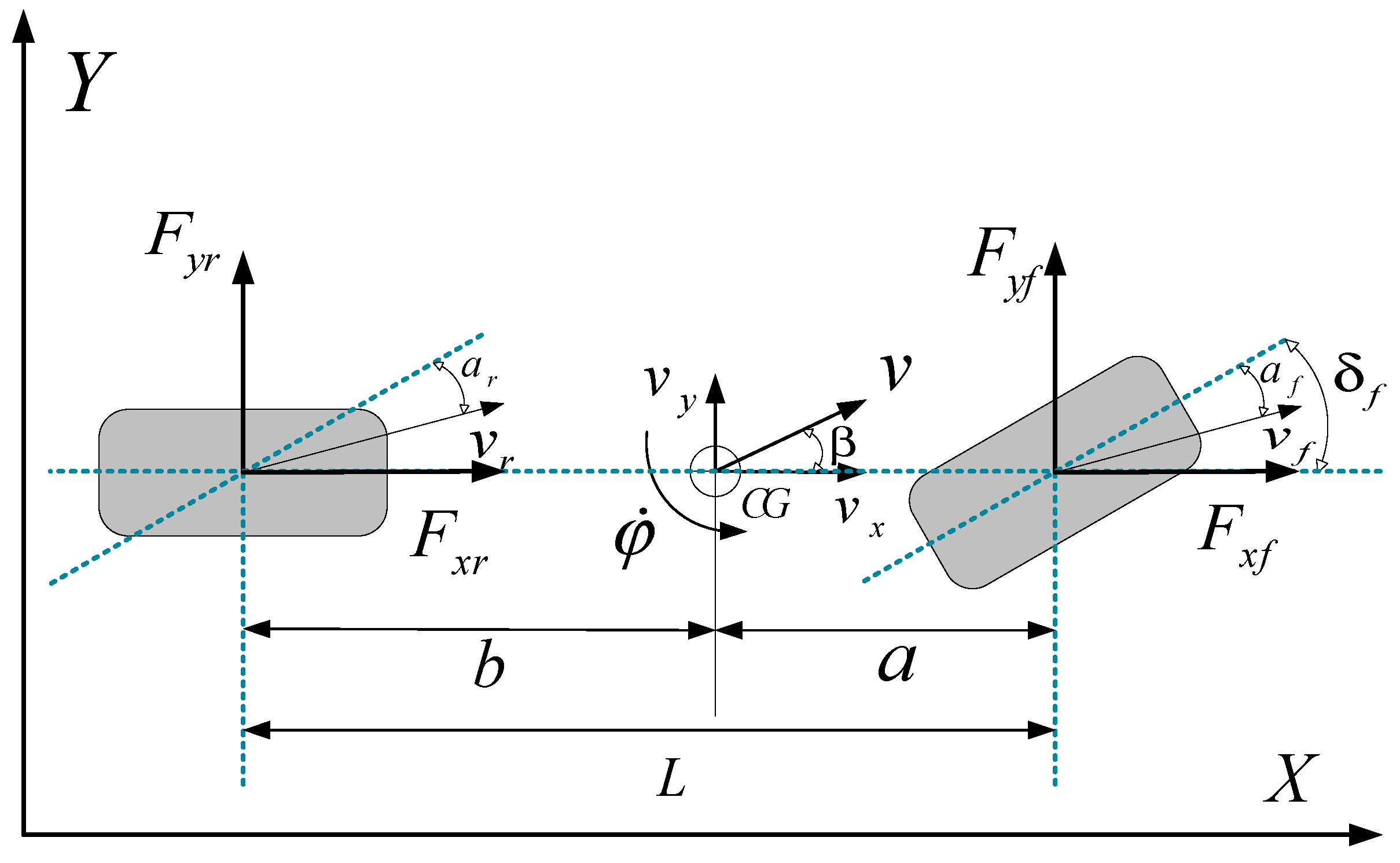
Based on the established three-degree-of-freedom vehicle model, the nonlinear system of the vehicle can be expressed in the form of the following differential equation:

$$\dot{x}(t)=f(x(t),u(t))x(t)\in \chi u(t)\in \Omega$$

(8)

where $f$ is the state transition function, $x(t)$ is the state variable of the system, $u(t)$ is the control variable of the system, $\chi \in R^n$ is the set of state variables, $n$ is the dimension of the state vector, $\Omega \in R^m$ is the set of control variables, and $m$ is the dimension of the control vector.

In this system, the state variables are selected as $x(t)={[v_y,v_x,\phi ,\dot{\phi },Y,X]}^T$, and the control variables are selected as $u(t)=[{\delta }_f]$.

The approximate linearization method, due to its simplicity in implementation and wide application range, has been widely used in the MPC field. Eventually, the linearized discrete system obtained is:

$$\begin{array}{l}x(k+1)=A_{k,t}x(k)+B_{k,t}x(k)+d_{k,t}(k)\\ A_{k,t}\in R^{n\times n},B_{k,t}\in R^{n\times m}\end{array}$$

(9)

The output equation of the nonlinear system is as follows:

$$\begin{array}{l}y(t)=h(x(t),u(t))\\ y(t)\in R^p,y(t)={[\phi ,Y]}^T\end{array}$$

(10)

which, $p$ is the dimension of the output vector

After linearizing and discretizing the output equation, the following equation can be obtained:

$$y(k)=C_{k,t}x(t)+D_{k,t}u(k)+e_{k,t}(k)$$

(11)

Based on the discretized system equation, the system output at time within the prediction time domain is recursively calculated as follows:

$$\begin{array}{l}Y(t)={\psi }_t\stackrel{⌢}{x}(t|t)+{\Theta }_t\Delta U(t)+{\Gamma }_t\Phi (t)+\Lambda (t)\\ Y(t)=\left[\begin{array}{c}y(t+1|t)\\ y(t+2|t)\\ ⋮\\ y\left(t+N_p|t\right)\end{array}\right],{\Psi }_t=\left[\begin{array}{c}{\stackrel{⌢}{C}}_{t+1,t}{\stackrel{⌢}{A}}_{t,t}\\ {\stackrel{⌢}{C}}_{t+2,t}{\stackrel{⌢}{A}}_{t+1,t}{\stackrel{⌢}{A}}_{t,t}\\ ⋮\\ {\stackrel{⌢}{C}}_{t+N_p,t}{\displaystyle \prod _{i=I}^{t+N_p-1}{\stackrel{⌢}{A}}_{i,t}}\end{array}\right]\\ {\Theta }_t=\left[\begin{array}{cccc}{\stackrel{⌢}{C}}_{t+1,t}{\stackrel{⌢}{B}}_{t,t}& {\stackrel{⌢}{D}}_{t+1,t}& \dots & 0_{p\times m}\\ {\stackrel{⌢}{C}}_{t+2,t}{\stackrel{⌢}{A}}_{t+1,t}{\stackrel{⌢}{B}}_{t,t}& {\stackrel{⌢}{C}}_{t+2,t}{\stackrel{⌢}{B}}_{t+1,t}& {\stackrel{⌢}{D}}_{t+2,t}& \ddots \\ ⋮& ⋮& \ddots & ⋮\\ {\stackrel{⌢}{C}}_{t+N_p,t}{\displaystyle \prod _{i=t+1}^{t+N_p-1}{\stackrel{⌢}{A}}_{i,t}}{\stackrel{⌢}{B}}_{t,t}& {\stackrel{⌢}{C}}_{t+H_p,t}{\displaystyle \prod _{i=t+2}^{t+N_p-1}{\stackrel{⌢}{A}}_{i,t}}{\stackrel{⌢}{B}}_{t+1,t}& \dots & {\stackrel{⌢}{C}}_{t+H_p,t}{\displaystyle \prod _{i=t+N_c}^{t+N_p-1}{\stackrel{⌢}{A}}_{i,t}}{\stackrel{⌢}{B}}_{t+N_c-1,t}\end{array}\right]\\ \Delta U(t)=\left[\begin{array}{c}\Delta u(t|t)\\ \Delta u(t+1|t)\\ ⋮\\ \Delta u\left(t+N_c-1|t\right)\end{array}\right],{\Gamma }_t=\left[\begin{array}{llll}{\stackrel{⌢}{C}}_{t+1,t}& { 0}_{p\times n}& \dots & { 0}_{p\times n}\\ {\stackrel{⌢}{C}}_{t+2,t}{\stackrel{⌢}{A}}_{t+1,t}& {\stackrel{⌢}{C}}_{t+2,t}& ⋮& \ddots \\ ⋮& ⋮& \ddots & ⋮\\ {\stackrel{⌢}{C}}_{t+N_p,t}{\displaystyle \prod _{i=t+1}^{t+N_p-1}}{\stackrel{⌢}{A}}_{i,t}& {\stackrel{⌢}{C}}_{t+H_p,t}{\displaystyle \prod _{i=t+2}^{t+N_p-1}{\stackrel{⌢}{A}}_{i,t}}& \dots & {\stackrel{⌢}{C}}_{t+H_p,t}\end{array}\right]\\ \Phi (t)=\left[\begin{array}{c}\stackrel{⌢}{d}(t+1|t)\\ \stackrel{⌢}{d}(t+2|t)\\ ⋮\\ \stackrel{⌢}{d}\left(t+N_p-1|t\right)\end{array}\right],\Lambda (t)=\left[\begin{array}{c}e(t+1|t)\\ e(t+2|t)\\ ⋮\\ e\left(t+N_p|t\right)\end{array}\right]\end{array}$$

(12)

In the core mechanism of MPC, the state tracking problem is transformed into a real-time solution process of the control sequence through the open-loop optimization framework. Based on the predicted output set of Formula (12), by introducing the quadratic norm penalty of the tracking error and weighted adjustment mechanism of the control input, the objective function with multi-objective optimization characteristics is constructed as follows:

$$\begin{array}{r}\hfill J(x(t),u(t-1),\Delta U(t),\epsilon )={\displaystyle \sum _{i=1}^{N_{\mathrm{p}}}{‖y_{\mathrm{tr}}(t+i|t)-y_{\mathrm{ref}}(t+i|t)‖}_Q^2}\\ \hfill +{\displaystyle \sum _{i=0}^{N_{\mathrm{c}}-1}\Vert \Delta u(}t+i|t){\Vert }_R^2+{\displaystyle \sum _{i=0}^{N_{\mathrm{c}}-1}\Vert u(}t+i|t){\Vert }_S^2+\rho {\epsilon }^2\end{array}$$

(13)

Which, $y_{\mathrm{ref}}$ represents the reference output quantity, and $\epsilon$ is the relaxation factor, $Q\in R^{p_y\times p_y},R\in R^{m\times m},S\in R^{m\times m}$, $\rho \in R$ denotes the weight matrix assigned to each term in the objective function. The first term penalizes the deviation between the system output and the reference output; the second term constrains the magnitude of the control increment to minimize control energy consumption; the third term incorporates a slack variable, enabling convergence to a suboptimal solution in cases where the optimization problem is initially infeasible.

In the trajectory tracking controller design process, ensuring driving safety, enhancing control performance, and maintaining system stability under complex working conditions require the imposition of necessary dynamic constraints on the vehicle. This is especially critical in application scenarios such as mining dump trucks, where high center of mass, heavy loads, and operation on unstructured road surfaces make the design of dynamic constraints particularly important.

Centroid lateral deflection angle and yaw rate constraints: Stability control for mining dump trucks fundamentally relies on strict regulation of key dynamic parameters. These constraints are specifically defined as [24]:

$$\begin{array}{l}\beta \le \arctan (0.02\mu g)\\ \dot{\phi }\le {\displaystyle \frac{\mu g}{v_x}}\end{array}$$

(14)

Steering system constraints: Due to the physical structural limitations of mining dump trucks, a steering limit exists. To prevent mechanical shock and actuator saturation, both the front wheel angle and its rate of change are constrained as follows:

$$\left\{\begin{array}{l}-{30}^{°}\le {\delta }_f\le {30}^{°}\\ -6^{°}\le \Delta {\delta }_f\le 6^{°}\end{array}\right.$$

(15)

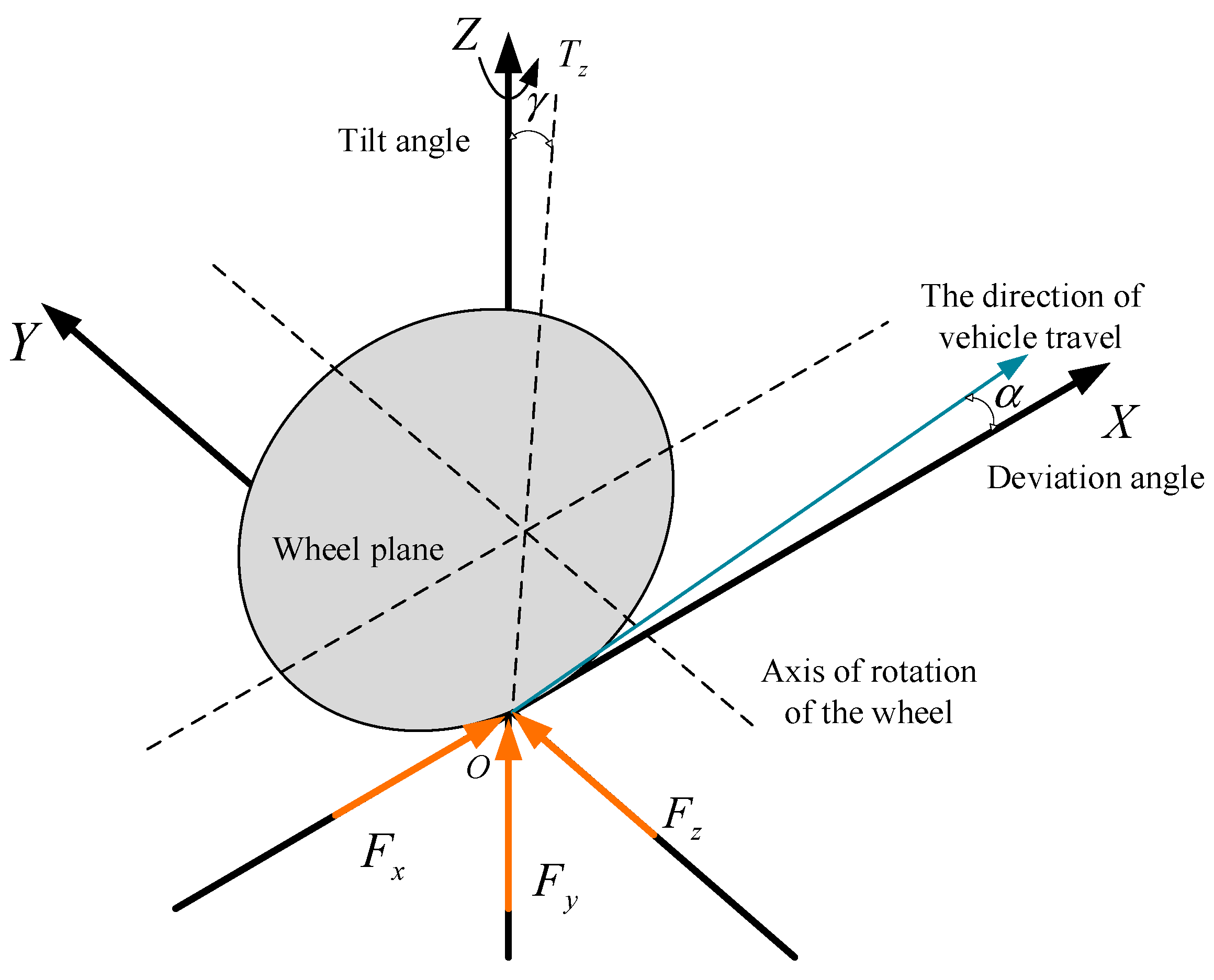
Attachment condition constraints: The dynamic performance of mining dump trucks is fundamentally limited by the friction characteristics of the tire–ground contact surface, and their motion state must satisfy the following attachment conditions:

$$\sqrt{a_x^2+a_y^2}\le \mu g$$

(16)

When the mining dump truck is traveling at a constant speed, the constraints can be simplified as:

$$\left|a_y\right|\le \mu g$$

(17)

In the MPC control algorithm, the $Q$ and $R$ matrices are used to adjust the weights of the state tracking error and the control input increment, respectively. A higher weight value indicates a greater emphasis by the controller on that particular term, resulting in a stronger tendency to reduce the corresponding error. The traditional MPC approach employs fixed weighting values, the selection of which typically relies on empirical trial and error. This method is not only time-consuming and labor-intensive but also prone to converging to local optima under complex operating conditions. 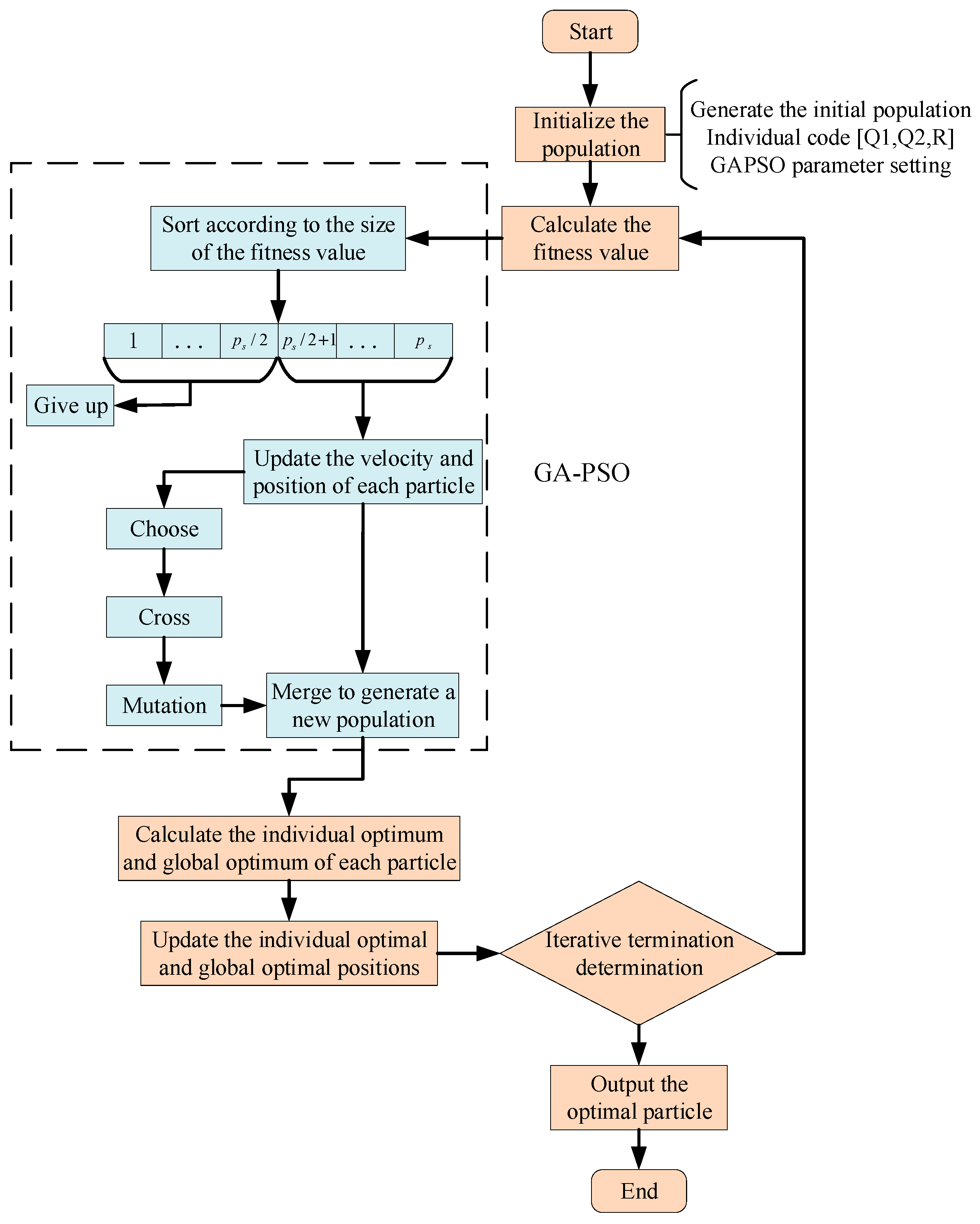However, achieving adaptive adjustment of the $Q$ and $R$ matrices in dynamically changing environments can significantly improve the stability, robustness, and response efficiency of the control system. Based on this analysis, this section proposes an adaptive weight MPC trajectory tracking controller that integrates the genetic algorithm and particle swarm optimization algorithm (GAPSO), as illustrated in Figure 3.

Genetic algorithms exhibit robust global search capabilities and are effective in avoiding convergence to local optima. The algorithm initiates with a randomly generated initial population, where each individual represents a potential solution to the problem. Through iterative application of genetic operators—including fitness evaluation, selection, crossover, and mutation—the population evolves toward improved solutions. Individuals exhibiting higher fitness values are more likely to be selected for reproduction. Crossover facilitates the exchange of genetic information between selected parents to produce offspring, while mutation introduces minor random alterations, thereby maintaining genetic diversity within the population. Over successive generations, the overall fitness of the population progressively improves, enabling the algorithm to converge to an optimal or near-optimal solution. The selection mechanism employed in the genetic algorithm in this study is as follows: 1. selection: Tournament selection with tournament size = 3; 2. Crossover: Simulated Binary Crossover (SBX) with probability $p_c=0.9$ and distribution index ${\eta }_c=20$; 3. Mutation: Polynomial mutation with probability $p_m=1/d$ (where $d=2$ is the number of decision variables: $q_y,q_{\psi }$ and distribution index ${\eta }_m=20$; 4. Population Merging: Initial population (50 individuals) is split: 25 for GA, 25 for PSO, After each generation, both subpopulations are merged into a single pool of 50, Fitness is evaluated for all 50; the best 25 become the next GA parent population, and the best 25 initialize PSO positions ($x_i$). PSO velocities ($v_i$) are randomly reinitialized within bounds. Personal/global bests are updated from the merged fitness ranking.

When applying the PSO algorithm, the values of parameters are of great significance, directly influencing the convergence, efficiency and quality of the final solution of the algorithm. The following is an analysis of the settings of relevant parameters in the PSO optimization algorithm.

Suppose in a $D$-dimensional search space, the number of particles is set as $m$. In this space, the position of the particle $i$ is denoted as $x_i=(x_{i1},x_{i2},\dots ,x_{iD})$, and its velocity is denoted as $v_i=(v_{i1},v_{i2},\dots ,v_{iD})$. The individual extremum of this particle is represented as $p_{besti}=(p_{i1},p_{i2},\dots ,p_{iD})$, and the global extremum is represented as $g_{best}=(g_1,g_2,\dots ,g_d)$. The velocity and position of each particle are updated iteratively through the following formulas.

$$\left\{\begin{array}{l}{x}_{t+1}=x_t+v_{t+1}\\ v_{t+1}=\omega v_t+c_1{r}_1(P_t-x_t)+c_2{r}_2(G_t-x_t)\end{array}\right.$$

(18)

where $i$ is the particle number, $d$ is the spatial dimension, $k$ is the number of iterations, $c_1,c_2$ are learning factors, $r_1,r_2$ are random numbers between 0 and 1, and $\omega$ is the inertia weight.

The setting of the population size needs to balance the search ability and computational efficiency. A smaller population size may limit the algorithm’s search ability and easily fall into a local optimal solution; while a larger population size can improve the global search ability, but it will increase the computation time. According to the complexity and dimension of the problem, the population size is usually set between 30 and 100.

The learning factors $c_1,c_2$ respectively represent the individual and population experience learning ability, controlling the intensity of particles learning towards the individual optimal position and the global optimal position. A larger $c_1$ value can enhance the particle’s learning ability towards the individual optimal position, and a larger $c_2$ value can enhance the particle’s learning ability towards the global optimal position. The value range is generally between 0 and 4.

The inertia weight controls the tendency of particles to maintain their original motion state. A larger value $\omega$ is conducive to global search, while a smaller value $\omega$ is beneficial for local search. The inertia weight typically adopts a linearly decreasing strategy, with an initial value set at 0.9 and a minimum value set at 0.4. This approach enables global search in the early stage of the algorithm and local search in the later stage, thereby enhancing the convergence accuracy of the algorithm. In this paper, $\omega$ is set as:

$$\omega (t)=0.9-0.5(iter/ite{r}_{\max })$$

(19)

where $iter$ represents the iteration number and $ite{r}_{\max }$ represents the maximum number of iterations.

To prevent particles from flying out of the solution space, it is also necessary to limit the maximum speed $v_{\max }$ of the particles. It is usually set to 10% to 20% of the particle’s variation range. A larger speed limit can enhance the exploration ability of the particles, but it may cause the particles to fly past the optimal solution; a smaller speed limit can improve the exploitation ability of the particles, but it may lead to a slower convergence speed of the algorithm.

During the iterative process of the GAPSO algorithm, the fitness function serves as the core evaluation mechanism and is used to quantitatively assess the control performance of each set of weight parameters $Q$ and $R$, along with their combinations. As a result, it directly influences the search direction and optimization efficiency of the algorithm. To meet the trajectory tracking requirements of distributed drive mining dump trucks, the fitness function must comprehensively balance tracking accuracy, control input smoothness, and system operational stability. The specific design is formulated as follows:

$$\begin{array}{ll}fitness& =w_Y\sqrt{\left({\displaystyle \sum _{k=1}^N{e_Y}^2}\right)/N}+w_{\phi }\sqrt{\left({\displaystyle \sum _{k=1}^N{e_{\phi }}^2}\right)/N}\\ \hspace{0.33em}& + w_{\delta }\sqrt{\left({\displaystyle \sum _{k=1}^N\Delta {\delta }^2}\right)/N}\end{array}$$

(20)

where $w_Y=1$, $w_{\phi }=1$, $w_{\delta }=0.1$ are the weights of the evaluation indicators, $e_Y$ is the lateral position tracking error, $e_{\phi }$ is the lateral swing Angle tracking error, $\Delta \delta$ is the rate of change in the front wheel Angle, and $N$ is the population size.

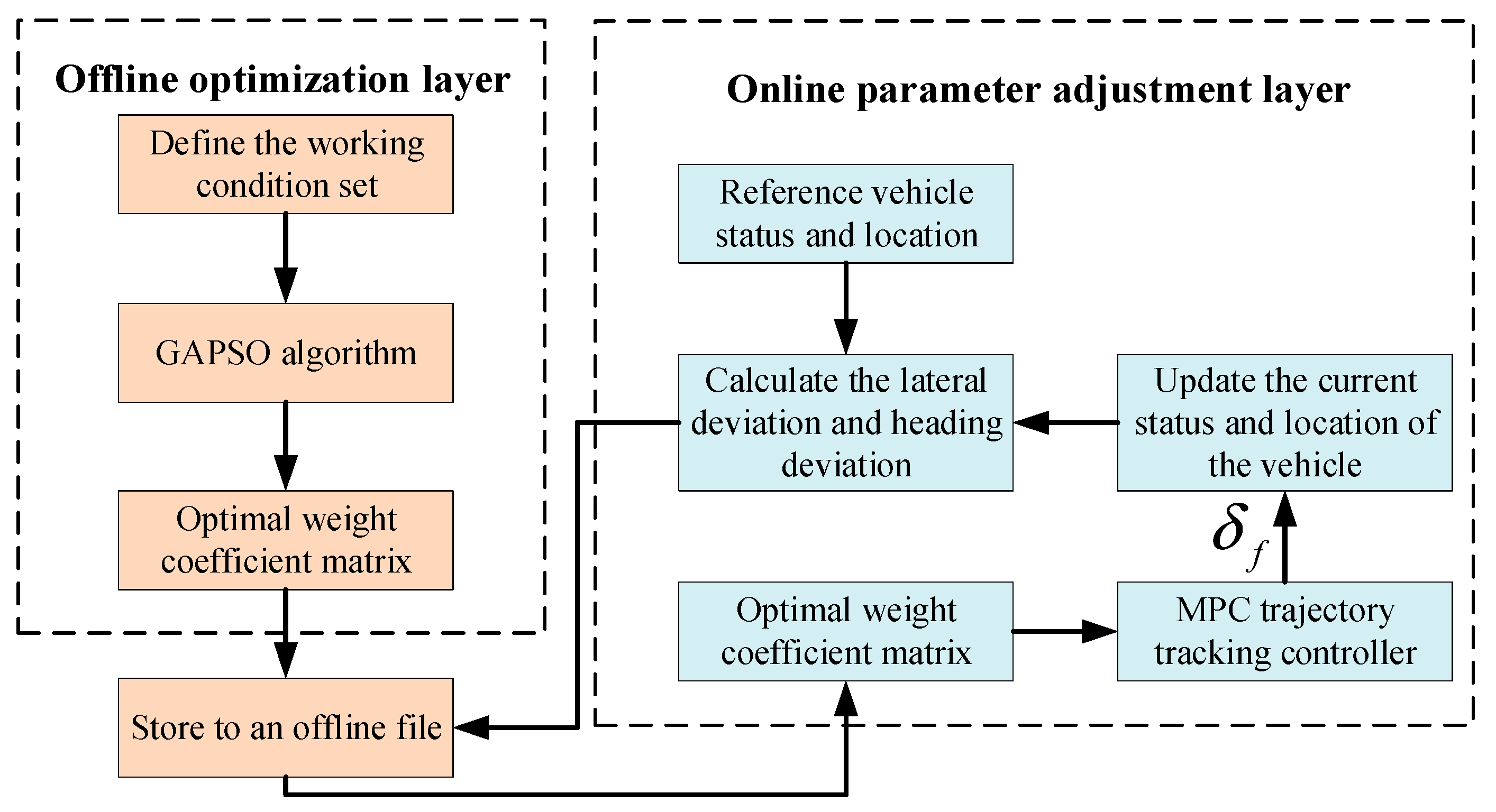
Given that the GAPSO fusion optimization algorithm requires substantial computational resources and time, this section proposes a hierarchical optimization architecture comprising an offline optimization layer and an online parameter adjustment layer, as illustrated in Figure 4. The offline database is constructed as follows: 1. Input Space: Lateral deviation $e_y\in [-1,1] m(step=0.1 m)$, Heading deviation $e_{\psi }\in [-0.5,0.5]\mathrm{rad}(step=0.05 \mathrm{rad})$; 2. Storage: For each grid point, store optimized ${q_y}^{*},{q_{\psi }}^{*}$ (scalar values, since $Q$ is diagonal with repeated entries); 3. Online Lookup: Bilinear interpolation is used for real-time queries. If $\left|e_y\right|>1$ or $\left|e_{\psi }\right|>0.5$, the nearest boundary values are used (saturation); With 441 precomputed entries, memory requirement is negligible (<10 KB), and interpolation adds minimal computational overhead. The primary function of the offline optimization layer is to employ the GAPSO fusion algorithm to compute the optimal state weight matrix and control weight matrix under various lateral and heading deviation conditions. These results are stored offline for subsequent query and retrieval by the online parameter adjustment layer. Building upon the traditional MPC trajectory tracking controller, the online parameter adjustment layer incorporates an adaptive mechanism for dynamically adjusting the state and control weight matrices. During the actual control process, the system retrieves the corresponding optimal weight matrix from the offline database based on the current heading and lateral deviations. Within each control cycle, the controller first acquires the vehicle’s current state and position information, then calculates the lateral and heading deviations relative to the reference trajectory. These error values are subsequently input into the offline optimization layer to search for the optimal weight coefficients, enabling dynamic adjustment of the $Q$ and $R$ matrices in the MPC controller. Once the weights are updated, the controller solves the optimization problem and generates control commands to be transmitted to the vehicle’s actuators. Upon receiving updated position information from the vehicle, the system proceeds to the next control cycle, repeating this process until all control tasks are completed.

4. Simulation Verification

In the MPC controller, in addition to the state weighting matrix $Q$ and control weighting matrix $R$, the selection of the prediction horizon $N_p$ and control horizon $N_c$ also plays a critical role in determining the system’s control performance, computational efficiency, and stability. A larger prediction horizon $N_p$ enhances the controller’s ability to anticipate future path deviations and dynamic variations, thereby improving overall control performance; however, it also increases computational complexity. In contrast, a smaller $N_p$ reduces computational load, but may compromise control effectiveness. A larger control horizon $N_c$ helps mitigate abrupt changes in control inputs and enhances disturbance rejection capabilities, yet it prolongs optimization solution time. Conversely, a smaller $N_c$ accelerates computation speed and improves adaptability to rapid dynamics, but may fail to fully exploit predictive information, potentially degrading control accuracy. Based on comprehensive considerations of system performance and engineering experience, this study selects a prediction horizon $N_p$ of 20 and a control horizon $N_c$ of 5.

Subsequently, the parameters of the GAPSO fusion algorithm were configured as follows: to balance global search capability and computational efficiency, the population size $N$ was set to 50; to optimize the trade-off between accuracy and runtime, the maximum number of iterations $ite{r}_{\max }$ was set to 100; the inertia weight $\omega$ was dynamically adjusted; both learning factors $c_1$ and $c_2$ were set to 2 to regulate particle learning intensity while maintaining algorithmic stability and convergence speed; mutation probability was implemented in two modes, with a high mutation probability $p_c$ set to 0.8 to enhance global exploration and accelerate the propagation of superior genes, and a low mutation probability $p_m$ 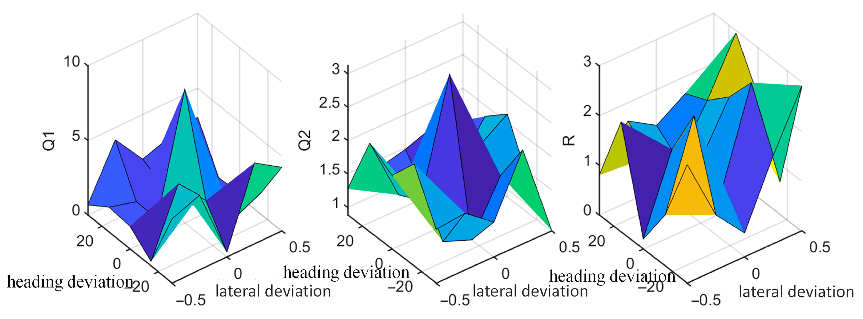set to 0.1 to preserve population diversity while ensuring acceptable convergence speed. The values of the state weight matrix and control weight matrix of the MPC trajectory tracking controller optimized by the GAPSO fusion algorithm under different lateral deviation and heading deviation conditions are shown in Figure 5. It can be seen from the figure that when the absolute value of the lateral deviation increases, the value of $Q1$ increases significantly, and when the absolute value of the heading deviation increases, the value of $Q2$ also increases significantly.

This section employs the standard double-lane change trajectory scenario to conduct simulation analysis and verification of the trajectory tracking control for distributed drive mining dump trucks. To comprehensively evaluate the control accuracy and system stability of the proposed MPC trajectory tracking controller optimized via the GAPSO fusion algorithm, three distinct operating conditions were established for comparative experimentation. Furthermore, to demonstrate the superiority of the proposed controller, comparative analyses were conducted against both the PSO-MPC-based controller (population = 50, iterations = 100, $c_1=c_2=2,\omega =(0.9\to 0.4)$) and the conventional MPC controller ($q_y=100,q_{\psi }=50,r_{\delta }=1$). To ensure fair comparison, all controllers share identical horizons, constraints, and vehicle models.

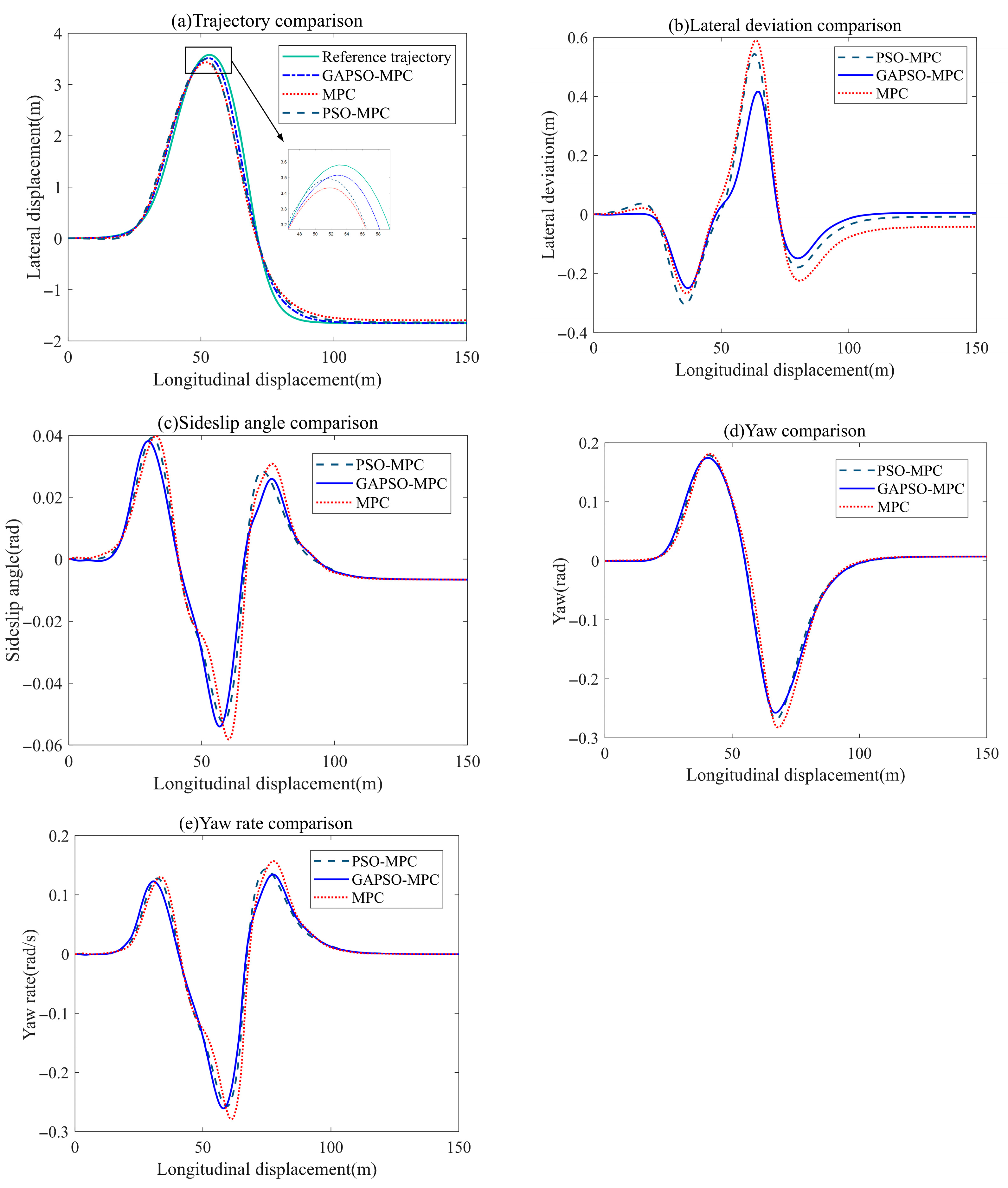
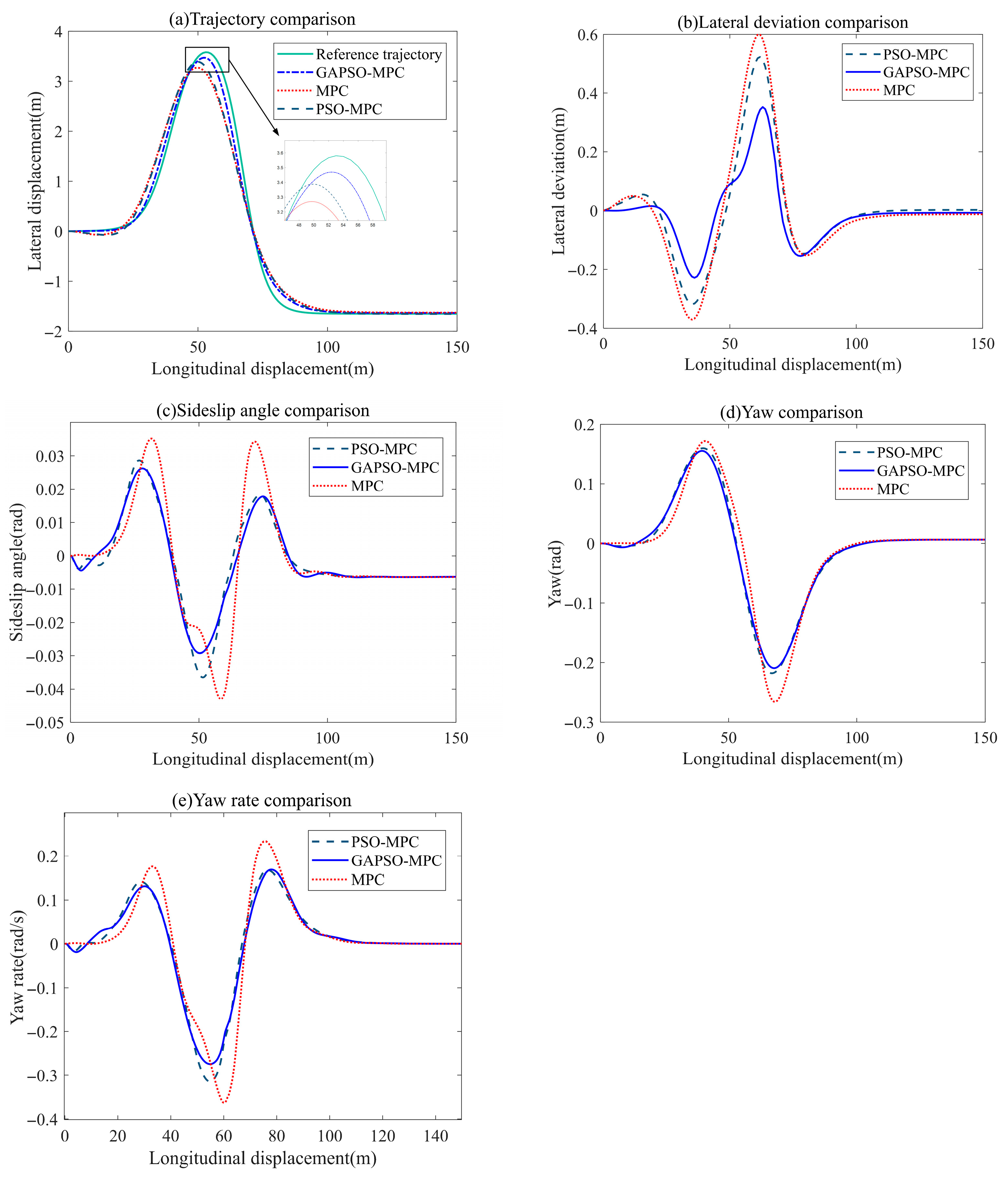
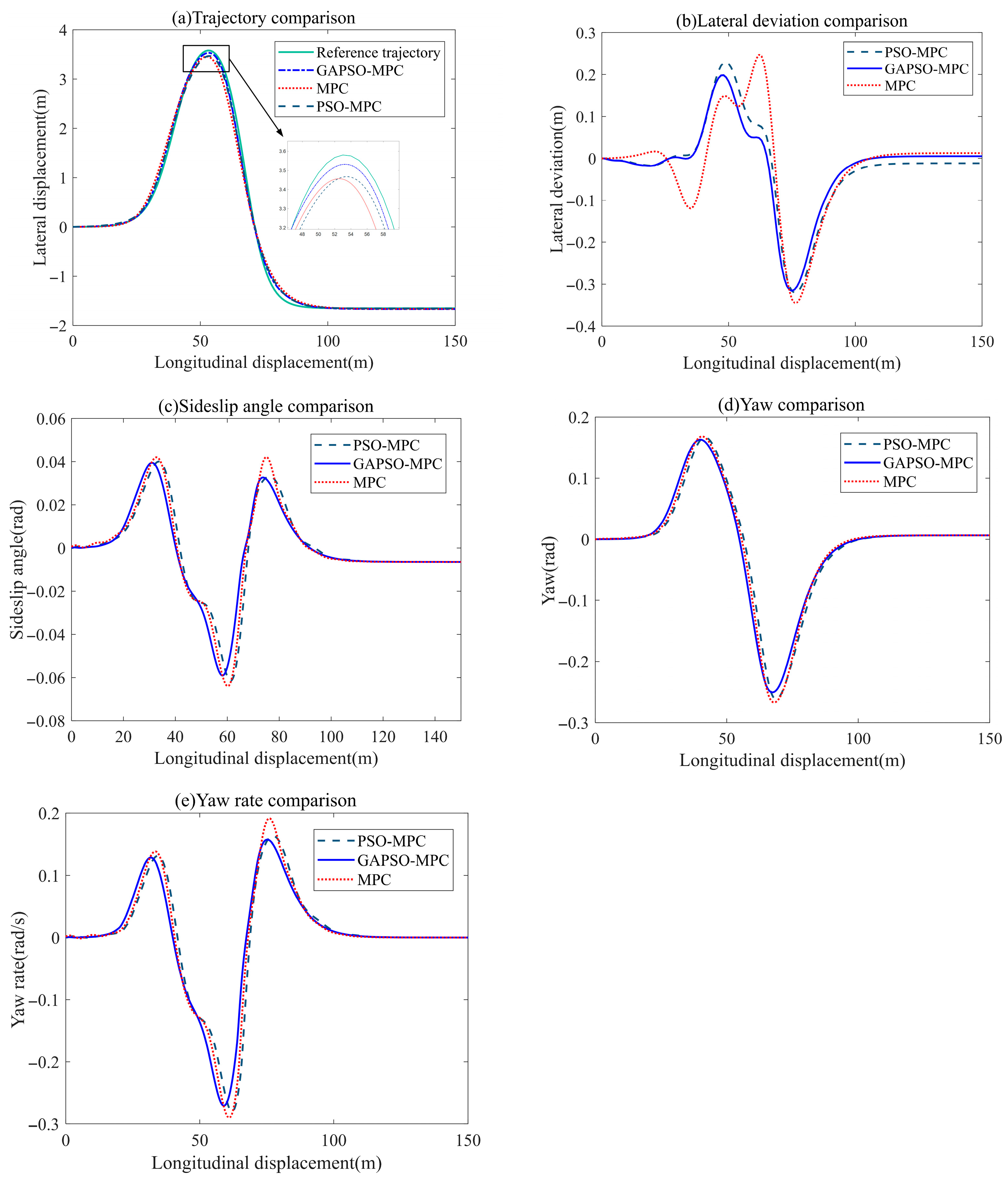
The corresponding simulation results are presented in Figure 6, Figure 7 and Figure 8. While only a single optimization run is presented per test condition due to computational limitations, preliminary trials indicate that the closed-loop RMSE exhibits low sensitivity (<2%) to random seed variations, consistent with practices in recent MPC-metaheuristic studies [25,26].

Condition 1 (Vehicle speed 18 km/h, road surface adhesion coefficient 0.7):

Under the working condition with an adhesion coefficient of 0.7 and a vehicle speed of 18 km/h, as shown in the trajectory comparison chart in Figure 6a and the lateral deviation comparison chart in Figure 6b, the GAPSO-MPC-based trajectory tracking controller exhibits a stronger capability to suppress steady-state deviation. The maximum lateral deviation of this controller is 0.244 m, with a root mean square error (RMSE) of 0.0719; whereas the PSO-MPC and traditional MPC controllers have maximum lateral deviations of 0.319 m and 0.352 m, respectively, with corresponding RMSEs of 0.0975 and 0.1033. It can be observed that compared to the other two controllers, the RMSE of the GAPSO-MPC controller is reduced by 26.26% and 30.4%, respectively. Moreover, as further illustrated in Figure 6c–e, the GAPSO-MPC controller effectively reduces fluctuations in the vehicle’s center of mass sideslip angle, yaw angle, and yaw rate during the trajectory tracking process, thereby significantly improving system tracking stability.

Condition 2 (Vehicle speed 18 km/h, road surface adhesion coefficient 0.3):

Under working conditions with a friction coefficient of 0.3 and a vehicle speed of 18 km/h, as shown in the trajectory comparison chart in Figure 7a and the lateral deviation comparison chart in Figure 7b, the GAPSO-MPC-based trajectory tracking controller exhibits superior steady-state deviation suppression capability and higher control accuracy. Although larger deviations may occur during the steering process, this controller can rapidly converge the system to the vicinity of the reference trajectory. Specifically, the maximum lateral deviation of the GAPSO-MPC controller is 0.4124 m, with a root mean square error (RMSE) of 0.0979; whereas the PSO-MPC and traditional MPC controllers exhibit maximum lateral deviations of 0.5456 m and 0.5869 m, respectively, with corresponding RMSEs of 0.1415 and 0.1564. It can be observed that compared to the other two controllers, the RMSE of the GAPSO-MPC controller is reduced by 30.81% and 37.4%, respectively. Moreover, as illustrated in Figure 7c–e, the GAPSO-MPC controller effectively suppresses fluctuations in key state variables such as the center of mass sideslip angle, yaw angle, and yaw rate during the trajectory tracking process, thereby significantly improving system tracking stability.

Further comparative analysis of the simulation results between working condition 2 and working condition 1 reveals that the tracking performance of all three controllers deteriorates under low adhesion conditions. This indicates that, with other factors held constant, a reduction in the road surface adhesion coefficient negatively affects trajectory tracking accuracy and compromises driving stability. Additionally, the changes in the root mean square error (RMSE) of lateral deviation across the two working conditions show that the RMSE increase for the GAPSO-MPC controller is 36.16%, for the PSO-MPC controller is 45.13%, and for the conventional MPC controller is 51.4%. These findings demonstrate that the GAPSO fusion optimization algorithm offers stronger adaptability in MPC parameter tuning, better handles challenges posed by varying road conditions, and delivers superior robustness and overall control performance.

Condition 3 (Vehicle speed 36 km/h, road surface adhesion coefficient 0.7):

Under the working conditions with an adhesion coefficient of 0.7 and a vehicle speed of 36 km/h, as shown in the trajectory comparison chart in Figure 8a and the lateral deviation comparison chart in Figure 8b, the GAPSO-MPC-based trajectory tracking controller demonstrates higher control accuracy. During the steering process, the vehicle trajectory tracking error exhibits certain transient fluctuations; however, this controller can rapidly converge the system to the vicinity of the reference trajectory, ensuring that all deviation values strictly satisfy the stability boundary constraints. Specifically, the maximum lateral deviation of the GAPSO-MPC controller is 0.3529 m, with a root mean square error (RMSE) of 0.0958; whereas the PSO-MPC and traditional MPC controllers have maximum lateral deviations of 0.5233 m and 0.5988 m, respectively, with corresponding RMSEs of 0.1458 and 0.1718. It can be observed that compared to the other two controllers, the RMSE of the GAPSO-MPC controller is reduced by 34.29% and 44.24%, respectively. As illustrated in Figure 8c–e, during the trajectory tracking process, the MPC controller optimized by the GAPSO fusion algorithm exhibits smaller responses in key state variables such as the center of mass sideslip angle, yaw angle, and yaw rate, thereby achieving better tracking stability performance. In conclusion, simulation results confirm that the GAPSO fusion optimization algorithm delivers excellent comprehensive performance in trajectory tracking control.

Further comparative analysis of the simulation results between working condition 3 and working condition 1 reveals that the tracking performance of all three controllers deteriorates under high-speed conditions. This indicates that, with other factors held constant, increased vehicle speed negatively affects trajectory tracking accuracy and compromises driving stability. Additionally, from the perspective of changes in the root mean square error (RMSE) of lateral deviation across the two working conditions, the RMSE increase for the GAPSO-MPC controller is 33.24%, for the PSO-MPC controller is 49.54%, and for the conventional MPC controller is 66.31%. These findings demonstrate that, under varying vehicle speeds, the GAPSO fusion optimization algorithm maintains strong adaptability and robustness in MPC parameter tuning, thereby delivering superior control performance.

5. Conclusions

This paper addresses the trajectory tracking control challenges encountered by distributed drive mining dump trucks in complex mining environments and proposes a model predictive control (MPC) strategy based on genetic-particle swarm optimization fusion (GAPSO). By constructing a hierarchical optimization architecture, the proposed strategy enables adaptive adjustment of the state weight matrix and control weight matrix in MPC, thereby enhancing control performance. Simulation results demonstrate that, compared with the PSO-MPC controller and the traditional MPC controller, the GAPSO-MPC controller reduces the root mean square error (RMSE) of trajectory tracking by 26.26% and 30.4%, 30.81% and 37.4%, and 34.29% and 44.24% under three typical working conditions, respectively. Experimental validation further confirms that the GAPSO-MPC-based trajectory tracking controller achieves high-precision tracking of the predefined trajectory across varying vehicle speeds and road adhesion coefficients, exhibiting superior control stability and enhanced environmental adaptability. In the subsequent research, the offline computational complexity of the control strategy proposed in this paper and its generalization ability for other trajectories or vehicles will be considered.