1. Introduction
Transportation plays a crucial role in national construction and development. A stable and efficient traffic management system forms the foundation for the normal transportation of production materials and the regular functioning of residents’ lives [
1,
2]. However, in recent years, the number of vehicles has been increasing annually, with the growth rate in some cities exceeding 10%, leading to severe urban road congestion [
3]. This not only affects residents’ normal travel, increases the probability of traffic accidents, but also severely restricts the development of urban areas [
4].
In order to alleviate traffic jams, governments around the world have taken a series of measures, such as widening roads, setting up traffic signals and implementing odd-even license plate restrictions. However, these methods cannot solve the problem fundamentally. The rapid development of information technology, computer science technology, and deep learning technology provides new ideas for solving this problem. Scientists have proposed the idea of intelligent control of traffic systems through high-speed data transmission technology and efficient artificial intelligence algorithms. Against this backdrop, Intelligent Transportation Systems (ITS) have emerged [
5,
6].
Among these, a viable strategy is to rapidly and accurately predict the traffic volume passing through a particular section or network of roads over a future period. The system, based on these predictions, can provide reasonable control measures, ultimately achieving the goal of alleviating or even eliminating traffic congestion. Therefore, traffic flow forecasting is of great significance to ITS [
7]. Scholars at home and abroad have conducted in-depth research on this issue and proposed a variety of prediction methods based on statistics, machine learning, and deep learning [
8].
In 2017, Google introduced the Transformer [
9], which achieved the best results in Natural Language Processing (NLP) tasks. Over time, this model has attracted the attention of many scholars and has been improved and widely applied in time series prediction problems such as Informer [
10], Reformer [
11], and Earthformer [
12]. However, the quadratic complexity of Scaled Dot Product Attention in time and memory has become a bottleneck for model scaling, and the dynamic output of the decoder carries the risk of error propagation and accumulation [
10,
11,
12,
13].
To address the above problems, this paper makes two improvements to the Transformer. Firstly, an Efficient Self-Attention mechanism is proposed, which reduces the dimensions of the key and value matrices through a linear layer, effectively reducing computational overhead. Secondly, a Generative Decoding mechanism is adopted in place of the original Dynamic Decoding mechanism. By outputting the prediction results of all steps at once, not only is the inference speed of the model accelerated, but the issues of error propagation and accumulation are also reduced. The new model is named EGFormer in this paper.
To verify the predictive performance of the new model, extensive experiments were conducted on two public datasets. The Recurrent Neural Networks(RNN) and its variants, as well as the Transformer and its improved model Informer, which are widely used in NLP problems and time series prediction tasks, were chosen as comparison models. In the analysis of experimental results, the authors conducted a detailed comparison with the results of the comparison models in terms of running time, prediction accuracy, and model robustness, and deeply analyzed the causes of the experimental results.
The results indicate that in traffic flow forecasting tasks, the newly proposed model can effectively extract non-linear features from the data. Compared with the models currently in widespread use, the EGFormer has higher prediction accuracy and shorter computation time.
The main contributions of this paper can be summarized as follows:
To address the quadratic complexity issue of Scaled Dot Product Attention in terms of time and memory, this paper proposes an Efficient Self-Attention mechanism. In this mechanism, the key and value matrices are projected into a lower-dimensional space through a linear layer, successfully reducing the computational overhead of the algorithm.
In the Transformer, a Generative Decoding mechanism is used to replace Dynamic Decoding. This operation not only accelerates the inference speed of the model but also effectively suppresses the problem of error propagation and accumulation.
This paper establishes the EGFormer based on the encoder–decoder structure and implements traffic flow forecasting tasks on this basis. The authors conducted extensive experiments using the public traffic flow datasets Pems04 and Pems08 to verify the performance of the model. The experimental results demonstrate the superiority of the model.
2. Preliminary
2.1. Multi-Head Self-Attention Mechanism
In 2017, the Google team proposed the Transformer based on the Self-Attention mechanism, achieving state-of-the-art results in the NLP field and attracting the interest of numerous scholars at home and abroad. In this paper, for convenience, the author only provides a brief introduction to the Self-Attention mechanism. The specific details of the Transformer can be found in literature [
9].
The Self-Attention mechanism is primarily used to learn the correlations between tokens in a sequence. The values are linearly mapped to the output through the queries and keys , with the weights determined by the correlation between and . The computation process of the Attention mechanism can be divided into the following three steps:
Step 1: The correlation between
and
is calculated through Scaled Dot Product:
where
denotes the transpose of
;
is the dimension shared by the model.
Step 2: The
is normalized by row. To further highlight the differences between the correlations, the SoftMax operation is usually used:
Step 3: Multiply the normalized
by
to obtain the final attention result:
In addition, to learn more about the correlations between sequences, linear neural network layers with learnable parameters are typically used to map
,
, and
to different spaces and aggregate the attention results computed in each space. The final output is then passed through a linear layer to maintain the same dimensionality. This operation, an improvement on Self-Attention, is commonly referred to as the Multi-Head Attention mechanism. Specifically, its computation method is as follows:
where
denotes the number of heads.
represents the output result of the
-th Attention head;
,
,
and
are learnable parameters.
2.2. Related Work
The research on traffic flow forecasting can be traced back to the 1960s and 1970s. After more than half a century of development, various prediction methods have been continuously proposed and widely used in engineering practice. According to the model type, these methods can be categorized into three groups: prediction methods based on statistical theory, prediction methods based on machine learning, and prediction methods based on deep learning.
2.2.1. Prediction Methods Based on Statistical Theory
The History Average (HA) model is the initial model of traffic flow forecasting research, which predicts future traffic flow by a weighted average of historical data. Still, it has been gradually discarded by researchers due to its oversimplification and low prediction accuracy. The Autoregressive Integrated Moving Average (ARIMA) [
14,
15,
16] model and its variants are classical methods in traffic flow forecasting based on statistical theory. Ahmed et al. [
17] investigated highway traffic and occupancy time series using ARIMA and finally found that the best metrics for all datasets were found when the model was ARIMA (0,1,3). However, the model was limited by the assumption of smoothness of the time series. In addition, Kalman Filtering (KF) is also a prediction method based on statistical theory. Okutanil et al. [
18] proposed two methods based on KF and achieved better results in traffic flow forecasting. Xie et al. [
19] investigated the application of KF and Discrete Wavelet Transform (DWT) in short-term traffic flow forecasting, and found that the wavelet-Kalman Filter performs better than the traditional KF.
2.2.2. Prediction Methods Based on Machine Learning
Machine learning-based prediction methods are one of the important branches of traffic flow forecasting theory, mainly including Support Vector Regression (SVR) and K-Nearest Neighbor (KNN) as well as variants of these two models. Li et al. [
20] proposed a short-duration traffic flow forecasting model based on improved SVR and achieved the best results in the comparison model. Aiming at the difficulty of parameter selection and the improvement of prediction accuracy, Li et al. [
21] used the Artificial Bee Colony algorithm (ABC) to optimize the SVR parameters and achieved satisfactory results in the experiments. Lin et al. [
22] used a combination of SVR and KNN to predict traffic flow and demonstrated the superiority of the model through experiments. Liu et al. [
23] proposed a hybrid prediction model based on KNN and SVR features and found experimentally that the prediction accuracy of this model is better than that of traditional prediction models such as SVR.
2.2.3. Prediction Methods Based on Deep Learning
Deep learning models discard the analysis of complex physical principles and the derivation of mathematical formulas, and the optimal combination of parameters in the model is obtained through a large amount of data training. With the rapid development of computer arithmetic, the potential of this field in the prediction of traffic flow has been further explored.
Recurrent Neural Networks (RNN) [
24] and its variants, Gated Recurrent Unit (GRU) [
25,
26,
27,
28] and Long Short-Term Memory (LSTM) [
4,
29], are one of the commonly used methods for traffic flow forecasting, where the model progressively analyzes and models the data along the time axis during the training process. Venkatesan et al. [
30] proposed a prediction model based on CNN-LSTM, and the experimental results show that the model has better prediction performance. Yang [
31] proposed a traffic flow forecasting model based on Recurrent Convolutional Neural Network and achieved good prediction performance in the experimental results. However, these models place more weights on several time steps closer to the current moment and cannot focus well on more distant temporal information, so they perform poorly in long-time traffic flow forecasting and are prone to the problems of gradient vanishing and gradient explosion.
Graph Neural Network (GNN) is another method commonly used in traffic flow forecasting. This type of model can effectively improve the prediction accuracy by considering the sensors on the road as the nodes of the graph; the sensors speak of the connection relationship of the nodes, then modeling the traffic road network as a graph to model the spatial correlation, and then modeling the temporal correlation through networks such as RNN. Yu et al. [
32] proposed a framework of the Spatio-Temporal Graph Convolutional Networks (STGCN), which employs graph convolution and ordinary convolution to extract the spatial and temporal correlations of the traffic road network, respectively, and reduces the computational overhead of the model by Chebyshev polynomial approximation and 1st order approximation, finally verifying the superiority of the model through experiments. Guo et al. [
33] introduced the Attention mechanism into the STGCN model and proposed the Attention based Spatial-Temporal Graph Convolutional Networks (ASTGCN) model; the experimental results showed that the prediction performance of ASTGCN was better than that of STGCN and other traditional prediction models. However, these models require the researcher to have a good understanding of the spatial structure of the transportation road network, and the connectivity between nodes has a more significant impact on the prediction performance.
The Transformer-based method is one of the current research hotspots in traffic flow forecasting. Modeling the correlations in the sequences through the Attention mechanism in the model effectively exceeds the limitation of temporal distance, which allows the model to learn more information between the sequences, and the performance is also better in the task of long-time traffic flow forecasting. However, the quadratic time complexity of the Attention mechanism limits the model’s extension to longer time series. In response, many scholars have improved the Self-Attention mechanism in the Transformer model to better extend it to longer sequences of prediction tasks. Zhou et al. [
10] proposed a ProbSparse Self-Attention mechanism that successfully reduces the time complexity to
. Wu et al. [
13] used a decompositional framework and an Auto-Correlated mechanism that reduces the time complexity to
and allows the model to focus on series-wise connections. Kitaev et al. [
11] used a hash Attention mechanism instead of the original Self-Attention mechanism in the Transformer, again reducing the time complexity to
. However, these models select only Top-k Attention values in the sequence, which may result in partial loss of information.
3. Methodology
Figure 1 shows the overall structure of the EGFormer. This model follows the Transformer framework and consists of two main parts: the encoder and the decoder. Both the encoder and the decoder are composed of one or more modules with the same structure but non-shared parameters. Each encoder module consists of an Efficient Self-Attention unit and a Feed-Forward Neural Network. Each decoder module first models the input information through a Masked Efficient Self-Attention unit, then facilitates information interaction between the encoder and decoder through an Efficient Attention mechanism, and finally ensures the data dimension remains unchanged through a Feed-Forward Neural Network. The output of the last decoder module is connected to a feed-forward layer to obtain the final output of the model. Furthermore, to prevent the model from experiencing the vanishing gradient problem as the network depth increases during computation, the model adds a residual block [
34,
35] and layer normalization operation [
36] after each computation.
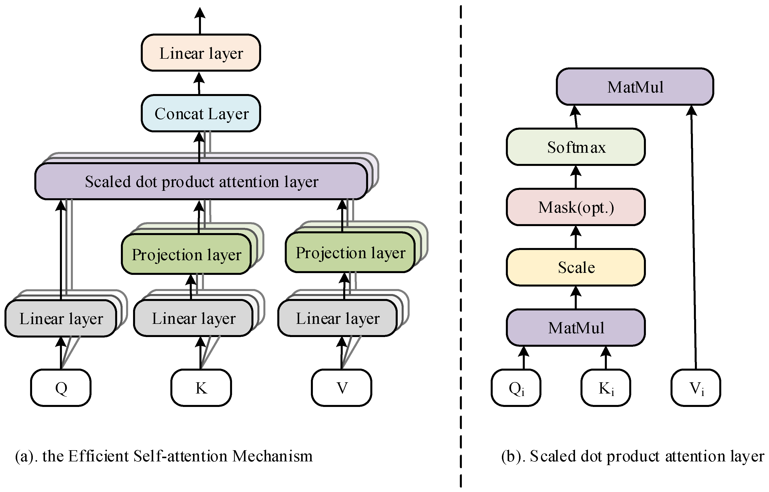
3.1. Efficient Self-Attention Mechanism
Equations (1)–(3) in the previous section describe the computation of the Self-Attention mechanism. In this process, two matrices and with sequence length and dimension need to be multiplied. However, in prediction tasks dealing with long sequences, the computation of Attention leads to huge storage requirements.
To address this problem, this paper proposes an Efficient Self-Attention mechanism, which reduces the dimensions of
and
by incorporating a linear projection matrix with learnable parameters in the process of calculating the Self-Attention, and thus realizes the purpose of reducing the computation of the model. Equation (6) shows the specific calculation method:
where
and
are the projection matrices of two learnable parameters.
is a custom parameter that can be set as a constant number smaller than
. In this way, the original dimensionality of
is maintained and the storage consumption is reduced.
Figure 2 shows the structure diagram of the Efficient Self-Attention mechanism.
3.2. Masked Efficient Self-Attention Mechanism
In the real world, the future is unknown, so a Masked Efficient Self-Attention mechanism is needed in the decoder structure. The mechanism is computed in essentially the same way as the Efficient Self-Attention mechanism, except that the future Attention score is set to 0 during the computation process. This means that the model can only learn knowledge in historical data and cannot learn any information from future data. In the formulaic expression, it is sufficient to perform the following operation on the correlation score
in Equation (1):
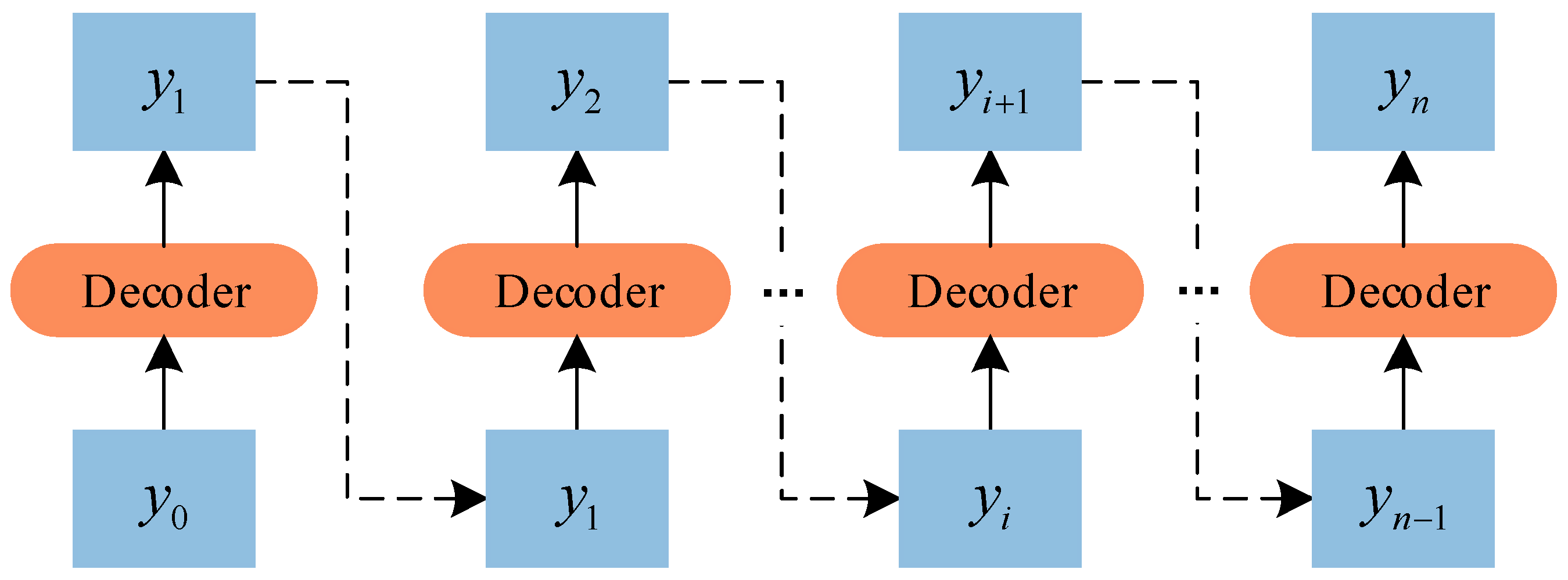
3.3. Generative Decoding Mechanism
During the inference process, the Transformer still follows the Dynamic Decoding in the RNN structure. Specifically, the output value
of the model at moment
depends not only on the inputs of the model, but is also influenced by the output value
of the previous
moments. This reasoning process can be visualized by the schematic diagram as
Figure 3 shows.
Usually, there is some error between the output values of the model and the actual values. Therefore, in the process of Transformer inference, with the increase of inference depth, the prediction error will gradually propagate forward, causing the problem of error accumulation. And the longer the prediction length of the task, the more serious this problem becomes. This is one of the major reasons why the Transformer does not work well in long- term traffic flow forecasting tasks.
For this aforementioned reason, this paper abandons the original Dynamic Decoding process and adopts a Generative Decoding mechanism. This mechanism outputs the predicted values of all time nodes at once during the model inference. Since the output results no longer depend on the previous output of the model, the problem of error accumulation can be effectively avoided, and the stability and accuracy of the model prediction is improved.
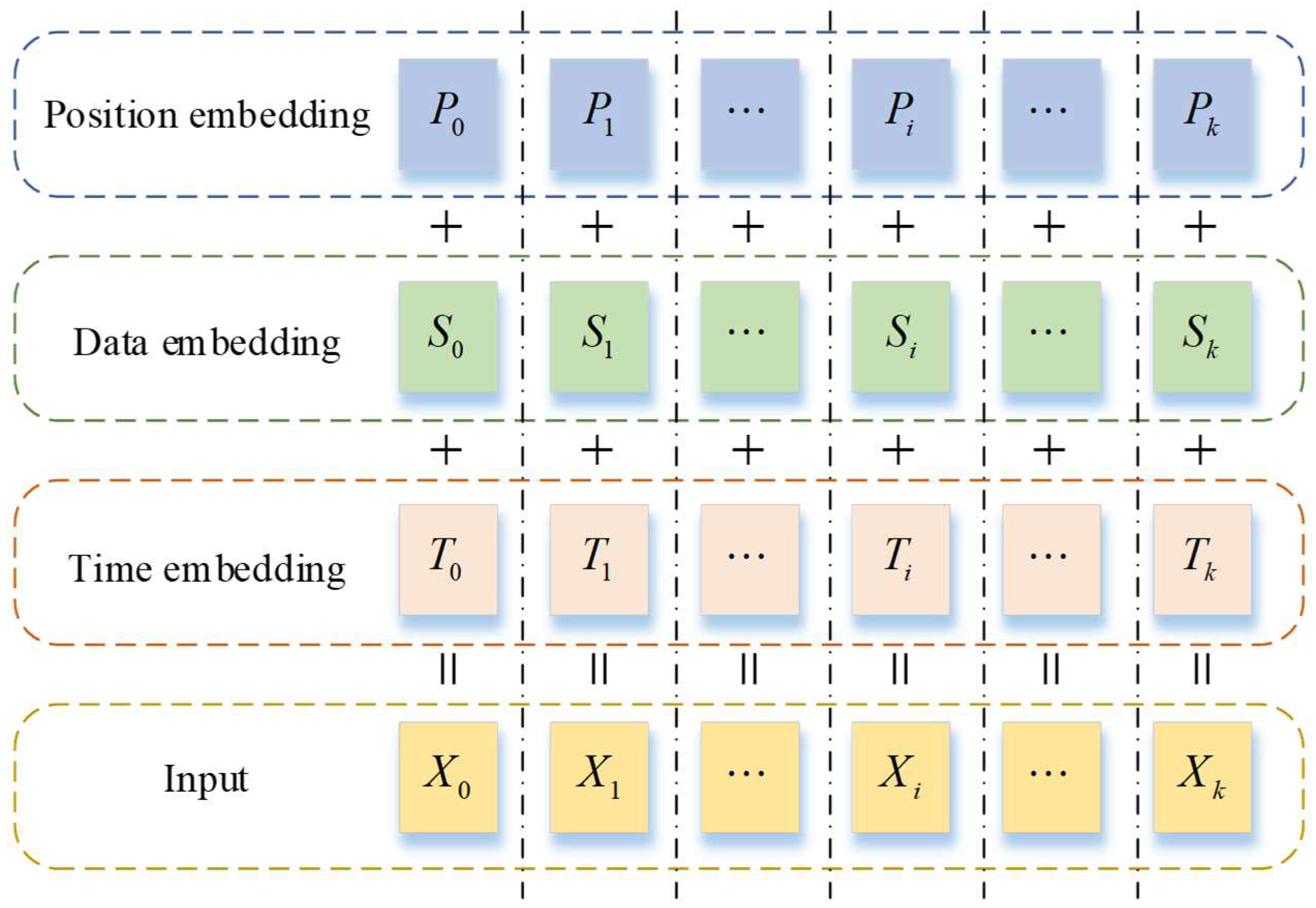
3.4. Data Embedding
The Attention mechanism overlooks the temporal order of data in the sequence, necessitating the embedding of additional positional information about the tokens in the model input. Concurrently, incorporating additional information beyond traffic flow data into the input can enhance the model’s learning capacity, thereby improving its predictive ability.
Therefore, the temporal information of the sequence was also embedded in the input sequence during the experiment. Consequently, the input data in the final model encoder and decoder consist of three components: traffic flow data, positional encoding information within the sequence, and temporal information, detailed as follows:
For data embedding, a one-dimensional convolution with a kernel size of 3 and a stride of 1 is employed.
For position embedding, this study adopts an absolute position embedding method alternating between sine and cosine as Equations (8) and (9) show:
where
denotes the position embedding value of
-th position;
denotes the current location.
As for time embedding, the authors employed convolutional operations to process data at five scales: year, month, day, hour, and minute, in order to extract relevant information from the time series.
Finally, the results of the three embeddings are added together to obtain the final input sequence as Equation (10) shows:
where
denotes the embedding result at the moment
.
,
, and
are the position embedding value, data embedding value, and time embedding value at the moment
.
In the Generative Decoding mechanism, Equation (11) is used to describe the input at the decoder end:
where
is the start sequence, which is the second half of the encoder input, and
is the part to be predicted, which retains only its time-encoded information at the time of input, and other information values are complemented by zeros.
is the length of the history sequence and
is the length of the predicted sequence.
Figure 4 illustrates the structure of the input data used in the model in this paper. This approach not only captures the changing trends among the traffic flow data but also effectively utilizes the dependencies between time and traffic flow data.
4. Experimental Setting
To validate the superiority of the EGFormer proposed in this paper, a large number of experiments were conducted. Before analyzing the results of these experiments, it is necessary to introduce the details involved in the experiments. In the following subsections, the authors will provide detailed information on aspects such as the experimental datasets, comparison models, evaluation metrics, experimental environment, and hyper-parameter settings.
4.1. Introduction to the Datasets
The experimental datasets used in this paper are derived from the public highway datasets Pems04 and Pems08, collected by the California Department of Transportation’s Performance Measurement System. The time interval for these two datasets is 5 min, meaning each sensor collects 288 data points per day. The Pems04 dataset includes data from 307 nodes in the San Francisco Bay Area network, collected from 1 January to 28 February 2018. The Pems08 dataset contains traffic data from 170 sensors in Los Angeles County, collected from 1 June to 31 July 2016. As this paper mainly focuses on the problem of single-node traffic flow forecasting, only the data from node 0 of each dataset were used in the experiments.
In the experiments, the datasets were divided in a ratio of 6:2:2.
Table 1 presents the specifics of this division.
To further enhance the stability of the trained model and the accuracy of the output results, it is necessary to normalize the traffic flow data prior to the experiments. This paper chose the min–max normalization method using the specific calculation method in Equation (12):
where
denotes the normalized data while
is the original data.
and
are the maximum and minimum values of the original data.
4.2. Compared Methods
To verify the predictive performance of EGFormer, we have selected several models that are widely used in the fields of NLP and time series prediction. These models include the RNN [
24] and its variants, GRU [
37] and LSTM [
38]. Moreover, given the improvements made to the Transformer [
9] in this study, the Transformer and its enhanced model, Informer [
10], were also chosen as comparison models. Brief introductions to each of these models are as follows:
RNN [
24]: The RNN models the correlation of data in a sequence along the time dimension, using hidden nodes within the model to retain the historical information of the sequence. With its simple mathematical principles, ease of understanding, and short training time, this model has been widely applied in NLP and short-term time series prediction tasks.
GRU [
37]: The GRU is an improvement on the RNN. It effectively addresses the issue of gradient decay during the training process by introducing the concept of gates into the model. Furthermore, it is capable of capturing changing relationships within time series.
LSTM [
38]: Similar to the GRU, the LSTM filters information in the time series through memory cells and gates in the model, thereby achieving effective information learning.
Transformer [
9]: The Transformer is a deep learning model based on the Attention mechanism proposed by the Google team. It initially achieved remarkable results in NLP tasks and has since been widely applied in multiple fields of Artificial Intelligence. This model is one of the important modeling frameworks in the field of time series prediction in recent years.
Informer [
10]: The Informer is an improved model proposed to address the shortcomings of the Transformer. It utilizes the ProbSparse Self-Attention mechanism, reducing the time and space complexity of the algorithm from
to
, without compromising the algorithm’s ability to extract information. Currently, the Informer is seeing increasing application in both short-term and long-term sequence prediction tasks.
4.3. Model Evaluation Metrics
In prediction tasks, it is common to use three metrics to verify the predictive performance of the model: Mean Absolute Error (MAE), Root Mean Square Error (RMSE), and Mean Absolute Percentage Error (MAPE). Equations (13)–(15) show the specific calculation formulas:
where
is the expected traffic flow data for the
-th sample, i.e., the real data.
denotes the predicted value of the model.
is the number of samples.
4.4. Experimental Environment
All experiments conducted in this study were executed on a Windows 10 platform, utilizing the widely popular PyTorch framework (version 1.13.1), Python version 3.9, and CUDA version 11.6.
4.5. Experimental Hyper-Parameters Setting
In neural networks, the configuration of model hyper-parameters plays a significant role in determining model performance. For instance, the number of hidden nodes in the model, if set excessively high, can slow down the training speed and increase the risk of overfitting. Conversely, if the number of hidden nodes is too low, the model may fail to sufficiently capture the internal information of the data, resulting in poor model performance. Thus, selecting appropriate model hyper-parameters is one of the key prerequisites for successful experimentation.
In the initial stage of the experiment, to identify reasonable hyper-parameters in the EGFormer and comparison models for optimal model prediction performance, a large number of experiments were conducted using a controlled variable method. Ultimately, the authors summarized the hyper-parameters for each model as follows.
(1) General hyper-parameters
General hyper-parameters refer to the model parameters that are included in all models during the experimental process.
In this study, the batch size was uniformly set to 32, and the Adam optimizer with a learning rate of 0.001 was used to train the models. The training process was halted after 50 iterations. The experimental task was to predict the traffic flow data of the next 12 time points through a historical sequence of 24 lengths. Given that the time interval of the dataset selected in this study is 5 min, this task can also be described as predicting the traffic flow data for the next hour based on the data from the past two hours.
(2) Other hyper-parameters
Due to the different structures and frameworks of each model, in addition to the aforementioned general hyper-parameters, each model also has some personalized hyper-parameters. The settings of these hyper-parameters in the experiments are briefly introduced below.
In the RNN, GRU, and LSTM, the number of internal hidden nodes was set to 64.
For the Transformer, Informer, and EGFormer, each model primarily consists of four encoder layers and two decoder layers. In the Multi-Head Attention mechanism, the model learns and aggregates feature information from different spaces through 8 heads. The vector dimensions were set to 64, and the number of nodes in the fully connected layer at the end of the decoder was 128. Moreover, to prevent model overfitting, dropout was employed in the experiments, with the dropout rate set to 0.05. To provide a more intuitive elucidation of the above content,
Appendix A presents a detailed analysis of the impact of the EGFormer’s hyper-parameters on prediction performance.
5. Results and Visualization
Based on the model structure introduced in
Section 3 and the parameters set in
Section 4, the authors conducted experimental validation of the performance of the EGFormer using data from node 0 of the Pems04 and Pems08 datasets. Simultaneously, models based on RNN (RNN, GRU, LSTM) and Transformer-based models (Transformer and Informer) were selected as comparison models. The experimental results and detailed analysis will be presented in the following sections.
5.1. Statistic of Model Prediction Performance
Table 2 presents the evaluation metrics of the prediction results and the average time consumed over 50 epochs during the training process for the six models. The authors specifically highlighted the best evaluation metrics (presented in bold) for the prediction task across the six models. The prediction horizons are 1, 6, and 12, respectively. The ‘Counter’ row shows the number of times each model achieved the best results.
The statistical results in
Table 2 indicate that in the prediction task for the Pems04 dataset, the EGFormer exhibits superior performance in all aspects except running time. Moreover, in the prediction task for the Pems08, the EGFormer also demonstrates its superiority in multiple tasks. The final statistical results show that the EGFormer model achieved the best values a total of 14 times in the two tasks, leading the count among the six models.
5.2. Comparison of Model Time Consummation
Training time is one of the crucial metrics for evaluating model performance. The authors calculated the average time spent on a single epoch during the training process for each model in the two prediction tasks;
Figure 5 depicts the results.
From
Figure 5, it can be observed that the training times of models based on RNN are relatively short, with RNN being the shortest, taking approximately 6 s. The GRU and LSTM, which introduce gate signals and memory cells into the RNN architecture, have increased computational steps compared to RNN. Experimental results show that compared to RNN, the training times of these two models increased by approximately 4% and 25.7%, respectively.
Meanwhile, Transformer-based models generally take more time, with the Transformer consuming the most time, being 4.4 and 3.9 times that of RNN on the two datasets, respectively. Although the Informer and EGFormer take less time than the Transformer, they still exceed 3 times the duration of the RNN. The reason for this phenomenon is the substantial time consumed by the Attention mechanism computation in these models.
To address the bottleneck of the squared time and memory complexity of the Scaled Dot Product Attention mechanism during the training process of the Transformer, the Informer and EGFormer models adopt the ProbSparse Self-Attention mechanism and Efficient Self-Attention mechanism, respectively, to reduce computational load. As a result, the training times of these two models are less than that of the Transformer. Qualitative calculations show that compared to the Transformer, the training times of Informer and EGFormer on the Pems04 dataset decreased by 6.81% and 27.78%, respectively, and on the Pems08 dataset, they decreased by 10.81% and 16.7%, respectively.
5.3. Loss of Validation Set
The predictive results of each model on the validation set will be discussed in detail in this section, focusing on the convergence ability of the models.
Figure 6 shows the convergence trends of the models.
The convergence curves intuitively reflect the convergence capabilities of each model. Experimental results indicate that the RNN has relatively poor convergence ability. As
Figure 6a shows with the red circles, after many iterations, there are still significant fluctuations. The reason for this phenomenon might be that the RNN is too simple to capture the complex functional relationships in long-term traffic flow sequences.
In contrast, the Attention mechanism in Transformer-based models breaks through the temporal distance of sequences and can better capture the changing relationships in the sequences. Therefore, their convergence ability is generally superior to that of RNN-based models.
Interestingly, the authors found that the EGFormer has the best convergence performance. As
Figure 6b shows, it tends to stabilize after about 10 epochs of training, without any significant rebound. The primary reason might be that the Efficient Self-Attention mechanism in the EGFormer successfully captures the functional relationships in the sequence.
5.4. Relationship between Prediction Step and Evaluation Metric
This section investigates the robustness of the models by observing the trends of various evaluation metrics of the model’s prediction results on the test set as the prediction step length changes.
Figure 7 intuitively shows the change in MAE, RMSE, and MAPE of each model as the prediction step length increases from 1 to 12. In
Figure 7, the horizontal axis ‘Horizon’ represents the prediction step length of the model, and the vertical axis represents the values of each evaluation metric.
It can be seen from
Figure 7 that as the prediction step length increases, the values of the three evaluation metrics also rise correspondingly. This phenomenon is consistent with the experimental results in
Table 2. The main reason is the uncertainty and unpredictability of the future. As the prediction step length increases, the model learns less information, and its predictive power for the future also weakens.
Among all models, the EGFormer exhibits good stability and superior performance. Specifically, its superiority is reflected in two aspects. First, compared to other models, the EGFormer model has lower evaluation metrics in all tasks. In fact, in the Pems04 traffic flow forecasting task, this model achieved the lowest score. Second, the growth rate of the EGFormer model’s metrics as the prediction step length increases is relatively slow, indicating that the model has strong stability.
5.5. Visualization of Prediction Results
This section will provide a visual representation of prediction results of the EGFormer, mainly including the model’s traffic flow forecasting within a day and a week. The following are the specific experimental results and their detailed analysis.
5.5.1. Visualization of Single-Day Prediction Results
Figure 8a displays the actual and predicted traffic flow data of the EGFormer on the Pems04 dataset for 17 February 2018, while
Figure 8b shows the model’s results on the Pems08 dataset for 20 June 2016. Here, ‘Ground’ represents the actual traffic flow data, and ‘Horizon 1’, ‘Horizon 6’, and ‘Horizon 12’, respectively, represent the results when the prediction steps are 1, 6, and 12.
It can be observed that the EGFormer can accurately perform prediction tasks under different prediction step lengths and scenarios, indicating that the model can capture the inherent information between data, demonstrating strong data tracking and mining capabilities.
5.5.2. Visualization of Weekly Prediction Results
Figure 9 intuitively presents the significant periodicity of traffic flow data and the EGFormer’s prediction results within a week. Specifically,
Figure 9a shows the prediction results for the Pems04 dataset from 17 February to 23 February 2018, and
Figure 9b displays the prediction results for the Pems08 dataset from 21 July to 27 July 2016.
It can be observed that the EGFormer can effectively extract the periodic information within the data, and the prediction results are able to follow the periodic changes of the actual traffic flow data well.
5.6. Extension and Migration of Models
This paper addresses the inadequacies of the Transformer in traffic flow forecasting tasks by proposing two improvement schemes. Verified by experiments, the improved algorithm demonstrates superiority in prediction tasks. In fact, the model proposed in this paper is not only applicable to traffic flow forecasting tasks but can also be widely used in other time series forecasting tasks, such as electricity load forecasting, stock forecasting, and disease spread forecasting, among others. During the model transfer process, it is necessary to adjust the hyper-parameters of the model appropriately according to the complexity and scale of the prediction task.
To verify the performance of the model in other domain time series prediction tasks, the authors chose the ETT dataset for validation experiments. This dataset includes the oil temperature data of power Transformers in two independent counties in China over two years, with a time granularity of 15 min. Each time point is composed of the oil temperature and six other Transformer features.
The specific hyperparameter settings in the experiment are as follows: the length of the historical sequence is 24, both the length of the label sequence and the prediction time sequence are set to 12, the encoding dimension of the input is 128, and 8 Efficient Attention heads are selected to learn information from different spaces. Since the time granularity of this dataset is larger than that of the Pems dataset, and the sequence changes are relatively simple, only two encoder layers and two decoder layers are set in the experiment to capture information in the time series.
Ultimately, the RMSE of the model’s prediction results on the ETT test dataset is 2.71, and the MAE is 2.18. These experimental results once again demonstrate the powerful capability of the proposed model in time series prediction tasks, and also show that the model has good scalability.
In
Appendix B of this paper, the authors visualized the model’s prediction results under this prediction task in order to more intuitively display the prediction results.
6. Conclusions
Accurate traffic flow forecasting is one of the key technologies in building ITS, providing a strong guarantee for the system to make correct decisions. However, due to the influence of various factors on traffic flow data, capturing the internal changes is quite challenging. Therefore, accurate prediction of traffic flow data remains a major challenge in the field of transportation.
The Transformer, with its powerful data learning ability due to the Attention mechanism, has performed exceptionally well in NLP and time series modeling tasks, far surpassing models such as RNN. However, in the task of traffic flow forecasting, researchers have identified two problems with the Transformer. On the one hand, the spatiotemporal quadratic complexity of the Attention mechanism leads to a significant amount of time and memory required during the model training process. On the other hand, the model’s inference process adopts a Dynamic Decoding approach, where the output of the previous moment is used as the input for the inference process of the next moment, leading to error propagation and accumulation.
This paper proposed two aspects to address these issues. Firstly, an Efficient Self-Attention mechanism is introduced, which adds linear mapping to the key and value matrices to reduce dimensions, thereby decreasing the computational overhead. Secondly, a Generative Decoding mechanism is used to replace the Dynamic Decoding process. This not only significantly accelerates the model training process but also effectively avoids the issues of error propagation and accumulation. Finally, through extensive experiments on two large public datasets, the superiority of the new model is demonstrated, indicating that the improvement strategies proposed in this paper are effective and feasible.
The main contribution of this paper is that it proposed a new improvement method for the Transformer, effectively solving some of the problems that the original model had in traffic flow forecasting tasks. The authors also point out in the research that traffic flow forecasting tasks based on Transformer-like algorithms (such as Transformer, Informer, Autoformer, etc.) have no significant differences in data processing and modeling frameworks from other time series prediction tasks in scenarios such as electricity, finance, and temperature. Therefore, this model can also be further extended to other time series prediction tasks.
Despite the achievements of this study, future research still needs to delve deeper. The authors’ subsequent research will focus on traffic flow forecasting tasks for road networks, while exploring further methods to sparsify the Attention mechanism. In addition, the introduction of Graph Convolutional Neural Network algorithms is considered, which allows for simultaneous modeling of the spatio-temporal correlation of traffic flow data based on the traffic network, further improving the prediction accuracy of the model.
Author Contributions
Conceptualization, W.C. and Z.Y.; methodology, Z.Y. and Q.Z.; software, Z.Y. and W.C.; validation, W.C. and P.X.; formal analysis, Z.Y., W.C. and M.L.; investigation, Z.Y. and W.C.; resources, Q.Z. and P.X.; data curation, Z.Y. and W.C.; writing—original draft preparation, Z.Y.; writing—review and editing, Z.Y. and W.C.; visualization, W.C. and Z.Y.; supervision, Q.Z. and P.X.; project administration, Q.Z. and P.X.; funding acquisition, Q.Z. and P.X.. All authors have read and agreed to the published version of the manuscript.
Funding
This research received no external funding.
Data Availability Statement
Publicly available datasets were analyzed in this study. The data can be found here:
http://pems.dot.ca.gov/, accessed on 9 April 2023.
Conflicts of Interest
The authors declare no conflicts of interest.
Appendix A. The Influence of Hyper-Parameters on Model Performance
In deep learning, hyper-parameters have a significant impact on the performance of the model and are one of the key factors for successful experiments. In
Section 4.5 of this paper, the authors describe the importance of hyper-parameters and provide a detailed introduction to the selection strategies and optimal combinations of models in the experiments. To provide a more intuitive illustration of this content, the authors have conducted a detailed analysis of how the EGFormer hyper-parameters impact prediction performance.
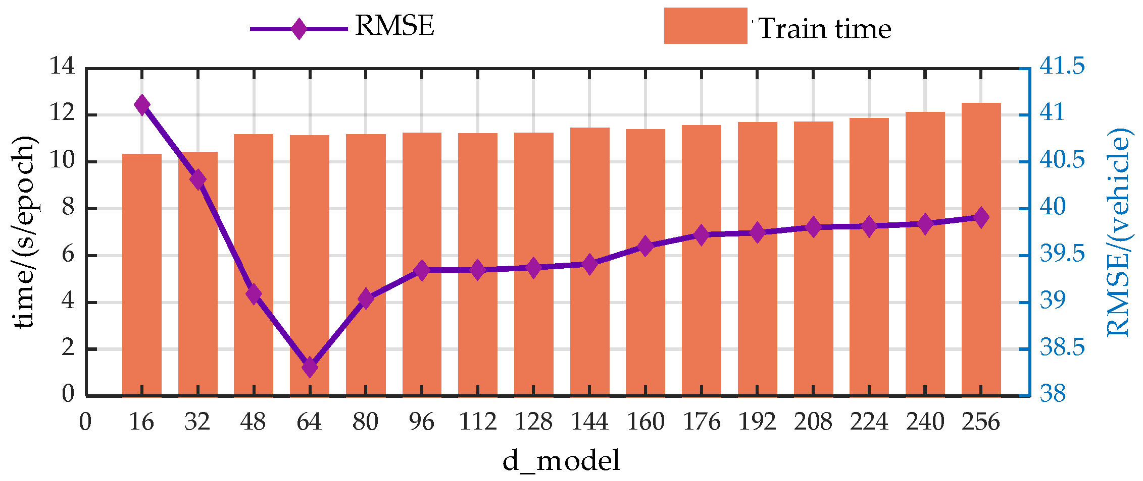
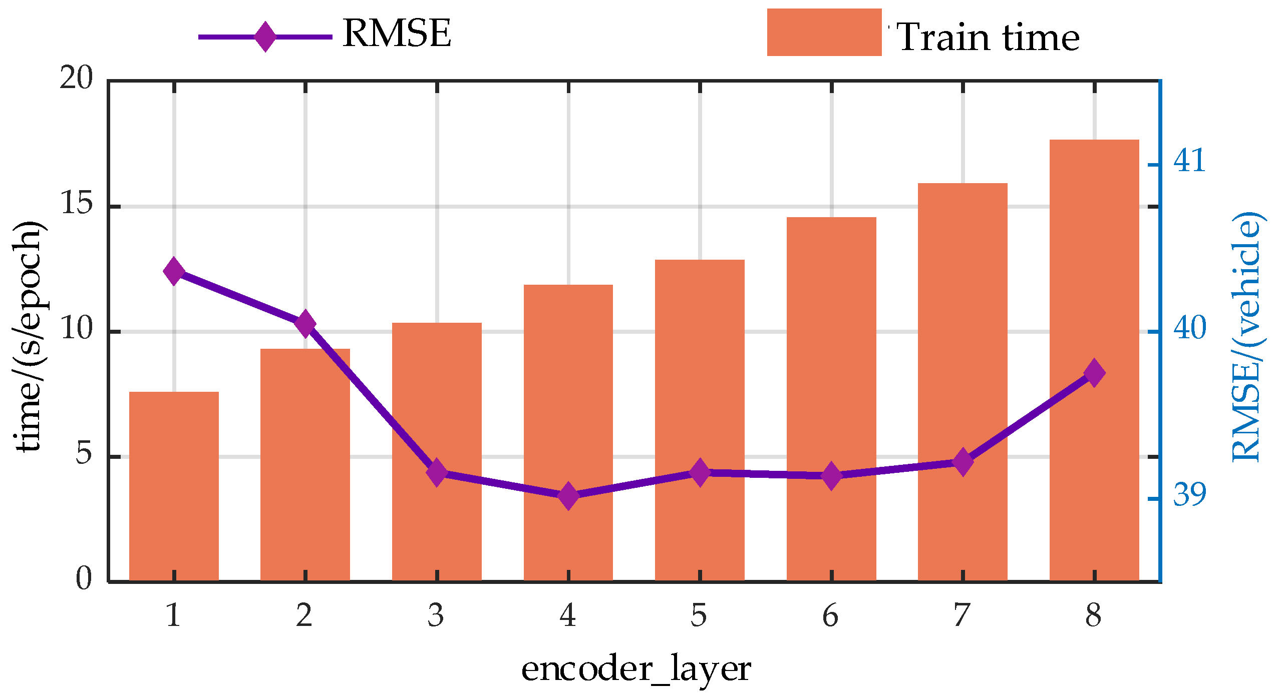
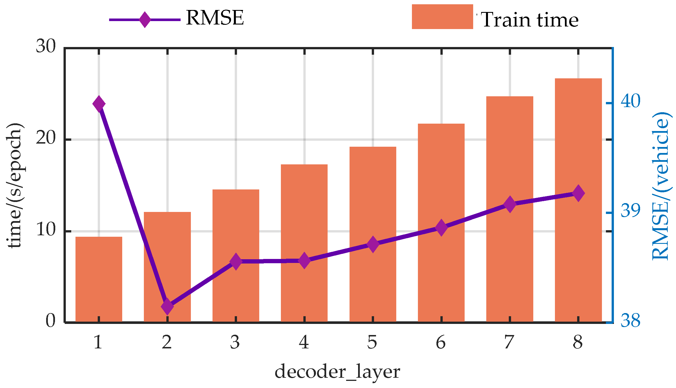
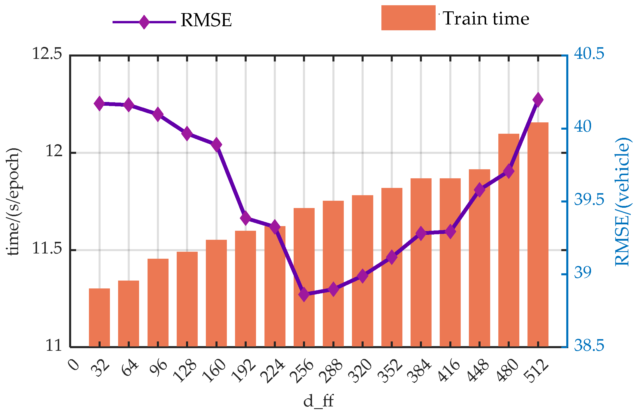
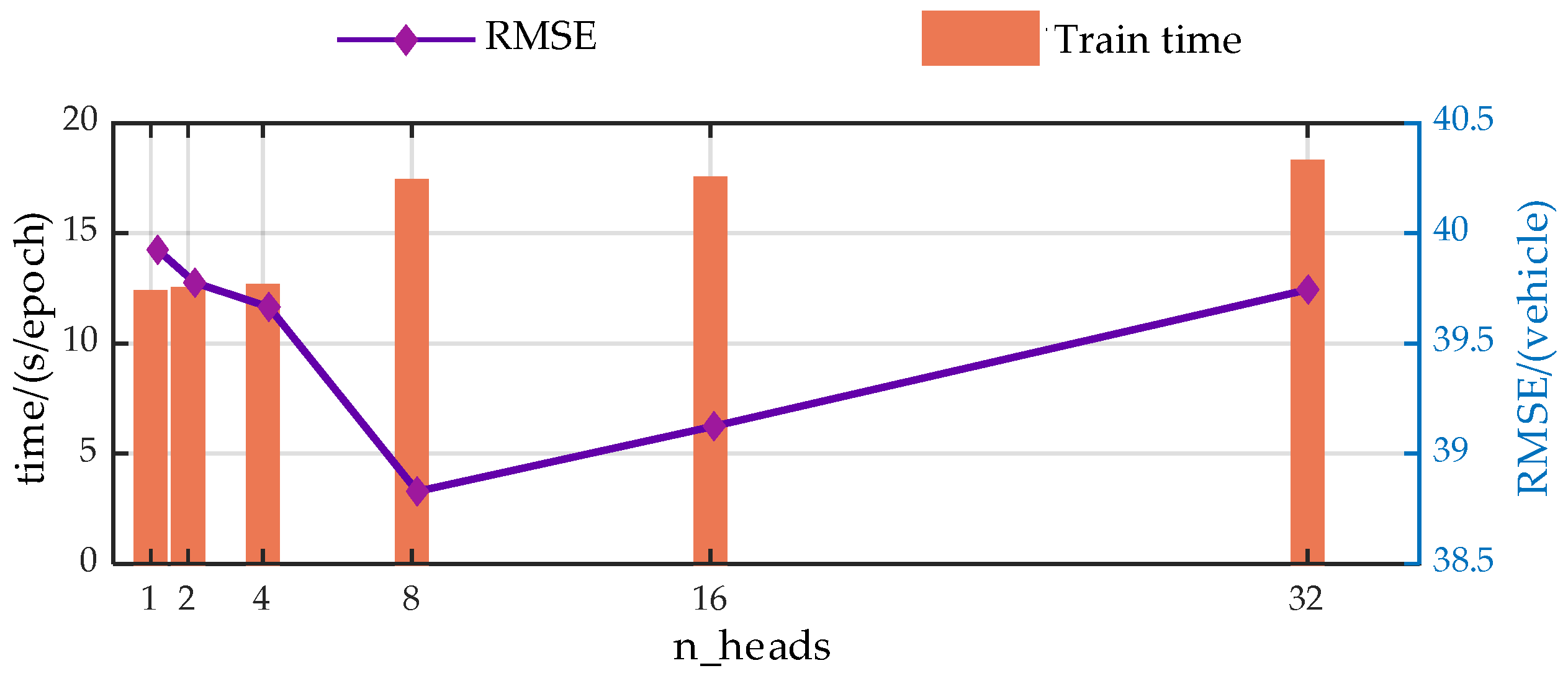
The authors discuss the impact of the input information encoding dimension (d_model), the number of heads in the Efficient Attention mechanism (n_heads), the number of encoder layers (encoder_layer), the number of decoder layers (decoder_layer), and the number of hidden nodes in the Feed-Forward Neural Network (d_ff) on the model’s prediction performance through a large number of experiments. In the experiments, each parameter value increases at equal intervals within a certain range, with RMSE and runtime being used as evaluation metrics.
For more intuitive analysis, the authors have plotted the trends of the EGFormer evaluation metrics with changes in the five hyper-parameters.
Figure A1,
Figure A2,
Figure A3,
Figure A4 and
Figure A5 show the visualization results.
Figure A1.
Trend analysis of prediction performance with variations in the d_model.
Figure A1.
Trend analysis of prediction performance with variations in the d_model.
Figure A2.
Trend analysis of prediction performance with variations in the n_heads.
Figure A2.
Trend analysis of prediction performance with variations in the n_heads.
Figure A3.
Trend analysis of prediction performance with variations in the encoder_layer.
Figure A3.
Trend analysis of prediction performance with variations in the encoder_layer.
Figure A4.
Trend analysis of prediction performance with variations in the decoder_layer.
Figure A4.
Trend analysis of prediction performance with variations in the decoder_layer.
Figure A5.
Trend analysis of prediction performance with variations in the d_ff.
Figure A5.
Trend analysis of prediction performance with variations in the d_ff.
Experimental results demonstrate that the hyper-parameters of the model have a significant impact on the predictive performance of the model.
From the perspective of prediction error, the predictive performance of the model presents similar trends with the changes of the hyper-parameters. As the model parameters increase, the predictive performance of the model first gradually decreases, which is due to the model gradually learning more information as the hyper-parameters increase. However, when exceeding a certain threshold, the performance of the model begins to deteriorate. This is primarily due to an overabundance of modules or hidden nodes causing the model to learn information that does not exist in the dataset during the training process, resulting in overfitting.
Additionally, from a temporal perspective, the time spent on each model training increases with the enlargement of the hyper-parameters. This is because when the hyperparameters increase, both the computational load and the storage requirements during the model training process increase, leading to a longer model training time.
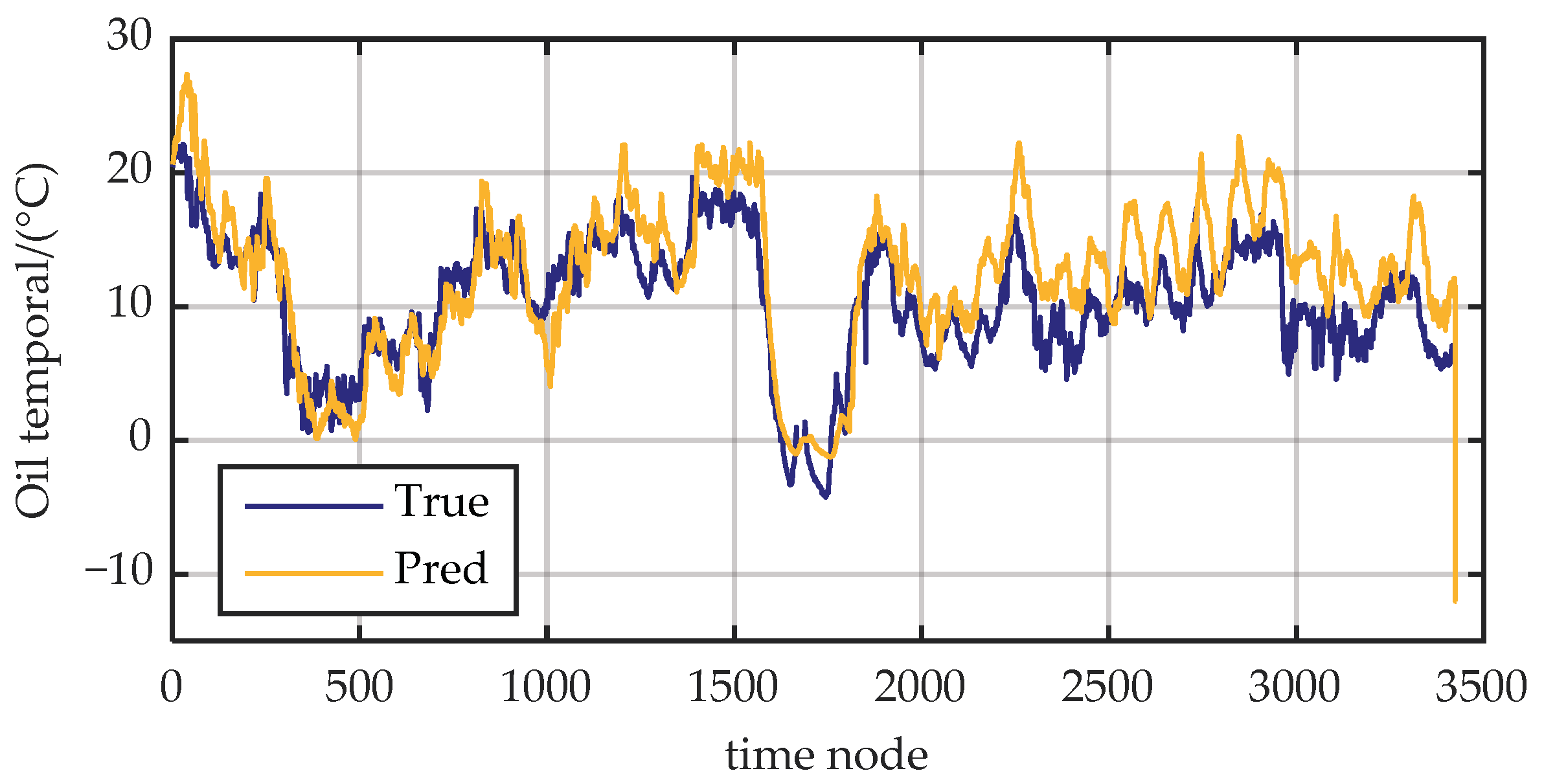
Appendix B. Visualization of the EGFormer’s Prediction Results on the ETT Dataset
Figure A6 presents the results of the EGFormer on the ETT dataset when the prediction step is 12. As can be seen from the figure, the model can follow the changing trend of oil temperature well. These results not only reiterate the superior predictive performance of the model but also demonstrate its excellent scalability, indicating that it can perform well in other prediction tasks.
Figure A6.
Prediction results of the model on the ETT dataset with a prediction step of 12.
Figure A6.
Prediction results of the model on the ETT dataset with a prediction step of 12.
References
- Alshehri, A.; Owais, M.; Gyani, J.; Aljarbou, M.; Alsulamy, S. Residual Neural Networks for Origin–Destination Trip Matrix Estimation from Traffic Sensor Information. Sustainability 2023, 15, 9881. [Google Scholar] [CrossRef]
- Owais, M. Traffic Sensor Location Problem: Three Decades of Research. Expert Syst. Appl. 2022, 208, 118134. [Google Scholar] [CrossRef]
- Zhao, W. Analysis of the Development of Intelligent Transportation Systems in China. Coast. Enterp. Sci. Technol. 2010, 4, 32–34. [Google Scholar]
- Ren, Y. Traffic Flow Forecasting Based on an Improved LSTM Network. Master’s Thesis, Dalian University of Technology, Shenyang, China, 2019. [Google Scholar]
- Lu, H.; Li, R. Developing Trend of ITS and Strategy Suggestions. J. Eng. Stud. 2014, 6, 6–19. [Google Scholar] [CrossRef]
- Hu, H.; Shen, J.; Huang, A. Research on the Sustainable Transportation Development and Intelligent Transport System. J. Transp. Syst. Eng. Inf. Technol. 2002, 2, 32–35. [Google Scholar]
- Li, Z.; Ge, H.; Chen, R. Traffic flow forecasting Based on BILSTM Model and Data Denoising Schemes. Chin. Phys. B 2022, 31, 040502-1–040502-10. [Google Scholar] [CrossRef]
- Jiang, W.; Luo, J. Graph Neural Network for Traffic Forecasting: A Survey. Expert Syst. Appl. 2022, 207, 117921.1–117921.28. [Google Scholar] [CrossRef]
- Ashish, V.; Noam, S.; Niki, P.; Jakob, U.; Llion, J.; Aidan, N.G.; Lukasz, K.; Illia, P. Attention Is All You Need. arXiv 2017, arXiv:1706.03762. [Google Scholar]
- Zhou, H.; Zhang, S.; Peng, J.; Zhang, S.; Li, J.; Xiong, H.; Zhang, W. Informer: Beyond Efficient Transformer for Long Sequence Time-Series Forecasting. arXiv 2020, arXiv:2012.07436. [Google Scholar] [CrossRef]
- Kitaev, N.; Kaiser, U.; Levskaya, A. Reformer: The Efficient Transformer. arXiv 2020, arXiv:2001.04451. [Google Scholar]
- Gao, Z.; Shi, X.; Wang, H.; Zhu, Y.; Wang, Y.; Li, M.; Yeung, D. Earthformer: Exploring Space-Time Transformers for Earth System Forecasting. arXiv 2022, arXiv:2207.05833. [Google Scholar]
- Wu, H.; Xu, J.; Wang, J.; Long, M. Autoformer: Decomposition Transformers with Auto-Correlation for Long-Term Series Forecasting. arXiv 2021, arXiv:2106.13008. [Google Scholar]
- Ahmed, M.; Cook, A. Analysis of Freeway Traffic Time-Series Data by Using Box-Jenkins Techniques. Transp. Res. Board 1979, 722, 1–9. [Google Scholar]
- Lippi, M.; Bertini, M.; Frasconi, P. Short-Term Traffic Flow Forecasting: An Experimental Comparison of Time-Series Analysis and Supervised Learning. IEEE Trans. Intell. Transp. Syst. 2013, 14, 871–882. [Google Scholar] [CrossRef]
- Tan, M.; Wong, S.; Xu, J.; Guan, Z.; Zhang, P. An Aggregation Approach to Short-Term Traffic flow forecasting. IEEE Trans. Intell. Transp. Syst. 2009, 10, 60–69. [Google Scholar]
- Ahmed, M.; Cook, A.; Borowski, R.; Cilliers, M.; May, A. Urban Systems Operations; Transportation Research Board: Washington, DC, USA, 1979. [Google Scholar]
- Okutani, I.; Stephanedes, Y. Dynamic Prediction of Traffic Volume through Kalman Filtering Theory. Transp. Res. Part B Methodol. 1984, 18, 1–11. [Google Scholar] [CrossRef]
- Xie, Y.; Zhang, Y.; Ye, Z. Short-Term Traffic Volume Forecasting using Kalman Filter with Discrete Wavelet Decomposition. Comput. -Aided Civ. Infrastruct. Eng. 2007, 22, 326–334. [Google Scholar] [CrossRef]
- Li, C.; Xu, P. Application on Traffic flow forecasting of Machine Learning in Intelligent Transportation. Neural Comput. Appl. 2021, 33, 613–624. [Google Scholar] [CrossRef]
- Li, C.; Zhang, H.; Zhang, H.; Liu, Y. Short-Term Traffic flow forecasting Algorithm by Support Vector Regression based on Artificial Bee Colony Optimization. ICIC Express Lett. 2019, 13, 475–482. [Google Scholar]
- Lin, G.; Lin, A.; Gu, D. Using Support Vector Regression and K-Nearest Neighbors for Short-Term Traffic flow forecasting based on Maximal Information Coefficient. Inf. Sci. 2022, 608, 517–531. [Google Scholar] [CrossRef]
- Liu, Z.; Du, W.; Yan, D.; Chai, G.; Guo, J. Short-Term Traffic Flow Forecasting Based on Combination of K -Nearest Neighbor and Support Vector Regression. J. Highw. Transp. Res. Dev. 2017, 34, 122–128. [Google Scholar] [CrossRef]
- Yu, D.; Qiu, S.; Zhou, H.; Wang, Z. Research on Short-Term Traffic flow forecasting of Intersections based on GRU-RNN Model. Highw. Eng. 2020, 45, 109–114. [Google Scholar]
- Feng, S.; Feng, C.; Shen, H. Research on Traffic flow forecasting based on K-Means and GRU. Comput. Technol. Dev. 2020, 30, 125–129. [Google Scholar]
- Lv, T. A Multi-Features Short-Term Traffic flow forecasting Method based on SDZ-GRU. Comput. Mod. 2019, 10, 60–65. [Google Scholar]
- Wang, S.; Shao, C.; Zhang, J.; Zheng, Y.; Meng, M. Traffic flow forecasting using Bi-Directional Gated Recurrent Unit Method. Urban Inform. 2022, 1. [Google Scholar] [CrossRef] [PubMed]
- Zhang, X.; Li, J. Traffic flow forecasting based on GRU-BP Combined Neural Network. J. Phys. Conf. Ser. 2021, 1873. [Google Scholar]
- Lin, F. Research on Short-Term Traffic Flow Forecasting Based on LSTM. Master’s Thesis, Chang’an University, Xi’an, China, 2020. [Google Scholar]
- Muthukumaran, V.; Natarajan, R.; Kaladevi, A.; Magesh, G.; Babu, S. Traffic flow forecasting in Inland Waterways of Assam Region Using Uncertain Spatiotemporal Correlative Features. Acta Geophys. 2022, 70, 2979–2990. [Google Scholar] [CrossRef]
- Yang, G. Research on Traffic Flow Forecasting Model Based on Recurrent Convolutional Neural Network. Master’s Thesis, Donghua University, Shanghai, China, 2022. [Google Scholar]
- Yu, B.; Yin, H.; Zhu, Z. Spatio-Temporal Graph Convolutional Networks: A Deep Learning Framework for Traffic Forecasting. In Proceedings of the 27th International Joint Conference on Artificial Intelligence, Stockholm, Sweden, 13–19 July 2018; pp. 3634–3640. [Google Scholar]
- Guo, S.; Lin, Y.; Feng, N.; Song, C.; Wan, H. Attention based Spatial-Temporal Graph Convolutional Networks for Traffic Flow Forecasting. In Proceedings of the Thirty-Third AAAI Conference on Artifical Intelligence, Honolulu, HI, USA, 27 January–1 February 2019; pp. 922–929. [Google Scholar]
- He, K.; Zhang, X.; Ren, S.; Sun, J. Deep Residual Learning for Image Recognition. In Proceedings of the 29th IEEE Conference on Computer Vision and Pattern Recognition (CVPR), Las Vegas, NV, USA, 26 June–1 July 2016; pp. 770–778. [Google Scholar]
- Sutskever, I.; Vinyals, O.; Le, Q. Sequence to Sequence Learning with Neural Networks. arXiv 2014, arXiv:1409.3215. [Google Scholar]
- Ba, J.; Kiros, J.; Hinton, G. Layer Normalization. arXiv 2016, arXiv:1607.06450v1. [Google Scholar]
- Cho, K.; Merrienboer, B.; Gulcehre, C.; Bahdanau, D.; Bougares, F.; Schwenk, H.; Bengio, Y. Learning Phrase Representations using RNN Encoder–Decoder for Statistical Machine Translation. Comput. Sci. 2014. [Google Scholar] [CrossRef]
- Gers, F.; Schmidhuber, J.; Cummins, F. Learning to Forget: Continual Prediction with LSTM. Neural Comput. 2000, 12, 2451–2471. [Google Scholar] [CrossRef] [PubMed]
| Disclaimer/Publisher’s Note: The statements, opinions and data contained in all publications are solely those of the individual author(s) and contributor(s) and not of MDPI and/or the editor(s). MDPI and/or the editor(s) disclaim responsibility for any injury to people or property resulting from any ideas, methods, instructions or products referred to in the content. |
© 2024 by the authors. Licensee MDPI, Basel, Switzerland. This article is an open access article distributed under the terms and conditions of the Creative Commons Attribution (CC BY) license (https://creativecommons.org/licenses/by/4.0/).


