Abstract
Distributed-drive vehicles utilize independent drive motors on the four-wheel hubs. The working conditions of the wheel-hub motors are so harsh that the motors are prone to failing under different driving conditions. This study addresses the impact of drive motor faults on vehicle performance, particularly on slippery roads where sudden faults can lead to accidents. A fault-tolerant control system integrating motor fault diagnosis and a direct yaw moment control (DYC) based fault-tolerant controller are proposed to ensure the stability of the vehicle during various motor faults. Due to the difficulty of identifying the parameters of the popular permanent magnet synchronous wheel hub motors (PMSMs), the system employs a model-free backpropagation neural network (BPNN)-based fault detector. Turn-to-turn short circuits, open-phase faults, and diamagnetic faults are considered in this research. The fault detector is trained offline and utilizes rotor speed and phase currents for online fault detection. The system assigns the torque outputs from both healthy and faulted motors based on fault categories using sliding mode control (SMC)-based DYC. Simulations with four-wheel electric vehicle models demonstrate the accuracy of the fault detector and the effectiveness of the fault-tolerant controller. The proposed system is prospective and has potential for the development of distributed electric vehicles.
1. Introductory
Transportation of people, goods, and services by vehicles is associated with problems such as energy shortages, environmental pollution, and traffic safety. Therefore, the development of electric vehicles (EVs), which are energy-saving, safe, and environmentally friendly, is an excellent solution for combating these problems [1,2,3]. Design ideas for electric vehicles are constantly changing and improving. An attractive drive form called “distributed independent drive” was recently proposed. It contains the advantages of fewer mechanical parts, a shorter transmission chain, and a flexible space arrangement. The distributed-drive electric vehicle (DDEV) has a motor installed in each wheel, which is called a wheel-hub motor. Through proper control, the drive forces and moment can be properly adjusted, thereby reducing the burden on the suspension system and improving the handling and responsiveness of the vehicle [4]. In addition, the distributed-drive vehicle can also improve its energy effectiveness [5]. Due to the advantages of DDEV, this research focuses on DDEV.
However, the operating conditions of the wheel-hub motor are very harsh. For example, the motor has poor heat dissipation due to the enclosure of the wheel; the motor suffers from severe vibration caused by the road and a rapid change in motor load. Therefore, the wheel-hub motor is prone to failure. If one of the motors fails and cannot provide proper torque output, it will significantly impact the vehicle’s stability. The vehicle will shift uncontrollably and vibrate swiftly [6]. In addition, on slippery roads, such as snow, ice, and mud roads, the friction factor of the road surface changes considerably, posing a more significant challenge to vehicle stability. For instance, Salimi et al. investigated the effect of different road conditions on the friction factor and vehicle tires. The results showed that the wet road decreases the friction factor and is detrimental to the stability of the vehicle [7]. As a result, appropriate fault-tolerant control strategies are required to maintain the stability and reliability of the vehicle in such conditions [8]. The basis of fault-tolerant control is fault diagnosis. It is a procedure to identify the position of the faulted motor and the type of fault. Under some electrical fault conditions (such as phase loss), the faulted motor can still provide limited torque output. Keeping such faulted motors working is necessary to prevent the overall drive forces and moment from significantly decreasing. The fault-tolerant controller can maintain the overall stability of the vehicle under acceptable, faulty conditions. It adjusts the healthy motors based on the results of the fault detector. It is only possible to assign the torque outputs of the rest of the healthy motors by identifying the faulted motors. Therefore, fault diagnosis for fault motor detection must come before vehicle-level fault-tolerant control.
Permanent magnet synchronous motors (PMSMs) are usually employed as hub motors for distributed electric vehicles. The common faults associated with PMSMs usually include the following aspects: open-circuit faults, turn-to-turn short-circuit faults, and demagnetization faults [9]. Open-circuit faults mean that the connection between the one-phase winding and the power source is lost and the current loop is opened due to vibration and other reasons such as loosening. These faults lead to electrical and mechanical faults and decrease output torque and load-carrying capacity [10]. Turn-to-turn short-circuit faults mean that the coils connect to each other and a closed loop for currents is created inside a phase winding due to high temperatures or other reasons. These faults increase stator winding current, overheat the motor, and vary the magnetic field and torque [11]. Torque outputs can be partially recovered by controlling the armature voltage of the motor to reduce the output torque fluctuation of the motor. The motor can still provide torque output with a few unpredicted deviations when the faults are electrical (including open circuit and turn-to-turn short circuit faults) [12]. The vehicle level controller amends the deviations through other healthy motors. Demagnetization faults are caused by high temperatures or pollution, resulting in the loss of magnetism in the permanent magnets. These faults result in an unstable flux density and change the electrical performance of the faulted PMSM. These faults are hard to detect and diagnose in terms of their severity [13]. Therefore, it is necessary to shut down the faulted motors with demagnetization faults and control the integral vehicle with other healthy motors.
Observer-based fault detectors have been among the most popular methods for electrical fault diagnosis in recent years. Zhang et al. proposed a fault-tolerant control method for steer-by-wire (SBW) based on the Kalman filtering technique to mitigate the adverse effects of steering angle sensor faults [14]. Bonci et al. investigated the application of a load torque observer based on the extended Kalman filter in diagnosing electric drives operating under non-stationary conditions [15]. The data-driven method are also a standard method for fault diagnosis. Typical methods include back propagation neural networks (BPNN); for instance, Kao et al. proposed an effective neural network-based algorithm for a series of faults of varying severity occurring in PMSMs operating at different speed ranges [16]. Wang et al. proposed a deep learning-based model called a multi-resolution and multi-sensor fusion network to diagnose electric motor faults by performing a multi-scale analysis of motor vibration and stator current signals [17]. Both methods are very efficient ways to achieve fault diagnosis. The parameters of PMSMs, such as flux density, inductance, and resistance, change with currents and temperatures, which are time-varying. This makes online parameter identification difficult. However, the data-driven methods can build the fault model automatically for fault detection based on sample input and output data without knowing the exact model parameters. As compared with deep learning approaches, BPNN is a data-driven method without the need for a million training data points. BPNN was adopted for this research.
Typical fault-tolerant controllers for vehicles often include logic-based or reinforcement-learning-based methods. Guo et al. proposed an adaptive fault-tolerant control method based on nonlinear vehicle dynamics and a new quadratic spacing strategy, which is used to ensure vehicle stability [18]. Deng et al. proposed a fault-tolerant control method based on deep reinforcement learning to consider the vehicle’s stability and the motor’s power consumption [19]. Logic-based methods depend more on experts as they require much practical experience. Reinforcement learning-based methods require much training in a virtual environment or in reality, which is costly and dangerous.
In addition, direct yaw moment control (DYC) is a standard vehicle stability control method. The controller adjusts the motion and driving stability of the vehicle by coordinating the brakes, engine output torques, and suspension system parameters of the vehicle. It has the advantages of fast speed, high precision, and low noise [20]. The main purpose of DYC is to give a slight direct yaw moment when the vehicle is steering and to improve the handling performance of the vehicle [21]. For example, in the case of steering at high speeds, if the torque from the right wheels reduces, the vehicle will turn to the right unpredicted. The DYC can reduce the output torque of the left wheels, increase the yaw moment to the left, and help the vehicle remain stable. For distributed-drive vehicles, when some motors fail, the stability of the direct motion of the vehicle can also be achieved by reasonably distributing the driving force of the remaining motors. DYC considers the performance and parameters of the whole vehicle. Many practical and theoretical analyses have confirmed the reliability of DYC in the application of distributed-drive vehicles. Therefore, DYC is believed to be adopted for fault-tolerant control of the vehicle. As a result, this study adopts the method of DYC for fault-tolerant control.
Various fault-tolerant control algorithms for distributed-drive EVs have been proposed and applied to DYC. Peng et al. proposed a robust model of predictive control (MPC) with a finite time for coordinated path tracking and DYC of distributed EVs [22]. Jin et al. proposed a robust fuzzy H ∞ control strategy by integrating a DYC system and active front steering to improve the lateral stability and handling performance of the vehicle [23]. Yue et al. investigated PMSM speed control using a direct torque control (DTC) scheme and space vector pulse width modulation (SVPWM) and designed a fractional order PID controller using fractional order calculus theory [24].
In contrast to the above algorithms, sliding mode control (SMC) has the advantages of fast response, insensitivity to parameter variations, no need for online system identification, disturbance tolerance, and simple physical implementation [25]. A sliding mode controller is a non-linear control method that defines a sliding mode surface that characterizes the state error of the system, and the system can adjust its outputs according to the changes in the sliding mode surface to gradually reduce the system error. There are also several applications of DYC on electric vehicles equipped with four in-wheel motors (IWMs). Li et al. proposed an adaptive SMC control scheme that is based on a novel stability index to represent the stability level quantitatively, thus improving handling and stability [26]. SMC has a tremendous advantage in hardware applications, especially in DYC control at the whole vehicle level [27]. Therefore, this research also adopts the SMC algorithm for fault-tolerant control.
The contributions and innovations of this paper include the following aspects: (1) It is an innovative attempt to study different motor fault types and their impact on vehicle performance, which can lay the foundation for a more in-depth study of the fault tolerance of electric vehicle systems. (2) It is a more forward-looking application of machine learning (particularly BPNN) based methods on motor fault detection in real working situations and not only considers the motor level but also the vehicle level. It also analyzes more efficient and feasible fault-tolerant strategies, providing a promising way of improving the reliability and safety of electric vehicles. (3) It is also an innovative attempt to propose a framework that combines motor fault diagnosis with vehicle-level fault-tolerant control, which is lacking in current research.
The remainder of this paper is assigned as follows: In Section 2, the vehicle model and both faulted and healthy motor models are developed. Section 3 shows the principles of the BPNN-based fault diagnosis and the SMC-based fault tolerance controller. Section 4 shows the simulation experimental results to verify their validity. Section 5 summarizes this paper and shows the possible work in the future.
2. Fault Modeling and Simulation
2.1. Modeling Distributed Drive Vehicles
2.1.1. 2-DOF Model
The 2-DOF model, as shown in Figure 1, describes the longitudinal speed, lateral speed,, and yaw rate of a vehicle based on tire dynamics. It provides an accurate motion model of the vehicle for reference. In this research, it serves as a reference for the fault-tolerant controller.
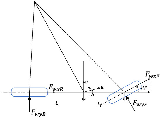
Figure 1.
2-DOF vehicle dynamics model.
The 2-DOF vehicle body dynamics equation is
where , , are the longitudinal speed, lateral speed, and yaw rate of the vehicle, respectively; represents the longitudinal force of the car; is the yaw moment to the vehicle; is the moment of inertia of the car, given by
where and are the longitudinal forces on the front and rear wheels of the car, respectively given by
where and are lateral forces for front and rear wheels; is the steering angle. and , are given by
where and are the lateral cornering stiffness of the front and rear wheels, respectively; and are the front and rear wheelbase, respectively.
2.1.2. 7-DOF Model
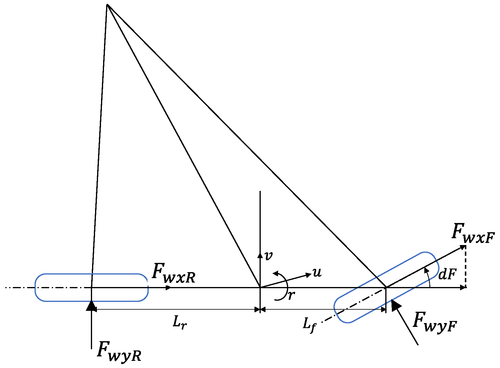
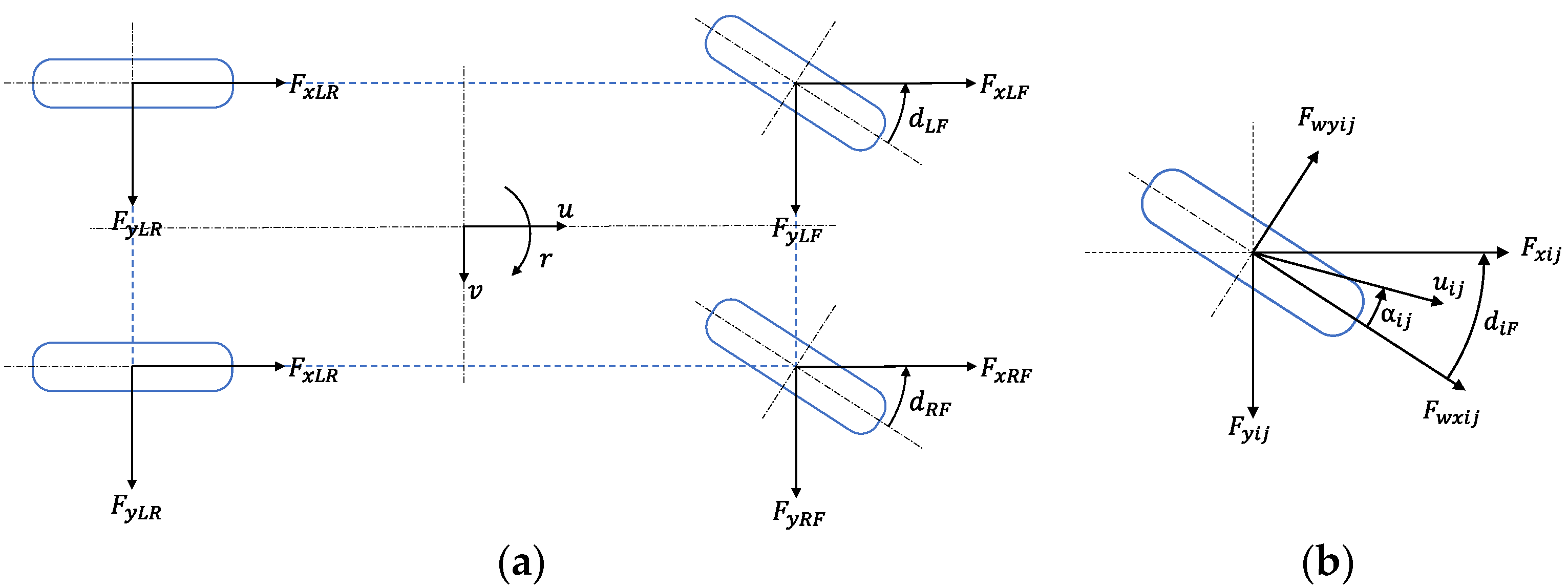
A 7-degree-of-freedom (7-DOF) model of the distributed electric vehicle is shown in Figure 2a. The forces on a single tire are shown in Figure 2b. This model works as the plant model of the distributed drive electric vehicle in the simulation environment in this research.
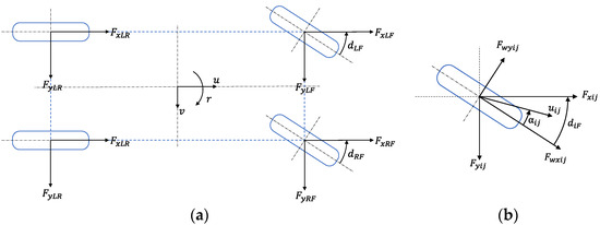
Figure 2.
7-DOF vehicle model (a) 7-DOF vehicle model (b) wheel model ( (right\left), (front\rear)).
The dynamic equation for the vehicle body is
where are the longitudinal speed, lateral speed, and yaw rate of the vehicle, respectively; , and are the longitudinal and lateral forces and the yaw moment of the vehicle, respectively; is the moment of inertia of the car, and represents the weight of the vehicle.
The longitudinal drive force is the sum of the longitudinal forces of the four wheels, and the air resistance is expressed as
where are the longitudinal forces of the left front, right front, left rear and right rear, wheels, respectively; is the air resistance.
The lateral force of the vehicle is the sum of the lateral forces of all four wheels, as shown in the equation of
where are the lateral forces of the left front, right front, left rear, and right rear wheels, respectively.
The yaw moment of the vehicle is defined as
where is the width of the vehicle; and are the front and rear wheelbase of the vehicle, respectively.
The longitudinal drive forces , , , and the lateral forces , , , of the wheels are defined by
where , , and are the drive force by the wheel hub motors, respectively; , , and are the lateral tire forces on left front, right front, left rear and right rear wheels, respectively; and are the steering angles of the left front and right front wheels, respectively, which is defined by
where is the front wheel steering angle. It is given by the driver in relation to the steering wheel angle. The relationship between these two angles is
where is the steering wheel angle given by the driver. The resistance is considered air resistance in this research is defined as
where is the initial air resistance; is the cross sectional area of the car; is the drag coefficient.
The lateral forces of each wheel, which are represented by, , and are defined by the side slip angles of the wheels as expressed by
where and are the cornering stiffness of front and rear tires, respectively.
The vertical forces of the wheels shall be used to determine whether the driving force can be provided based on the maximum fractional forces from the ground. The vertical forces of the vehicle are defined as
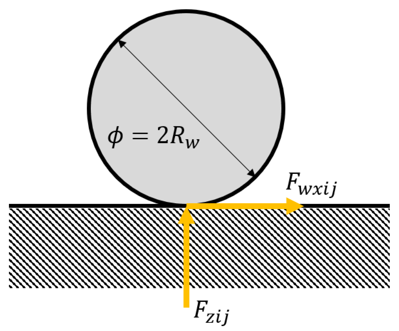
where are the vertical forces of the left front, right front, left rear, and right rear wheels, respectively; is the height of the center of gravity with respect to the ground. A single-wheel model is also defined in Figure 3.

Figure 3.
Forces on one tire.
The commonly used Magic Tire formula [15] that takes into account the longitudinal drive is [28].
where is the vertical load, B, C, and D are coefficients to be determined, is the slip rate of the tire, represent the tire position of left and right wheels, respectively; represent the tire position of front and rear wheels, respectively. The driving force works as not only the power source for the motion of the vehicle but also provides the driving torque. The values of B, C, and D for normal roads are listed in Table 1.

Table 1.
Coefficients of different road surfaces.
3. Fault Tolerance Control
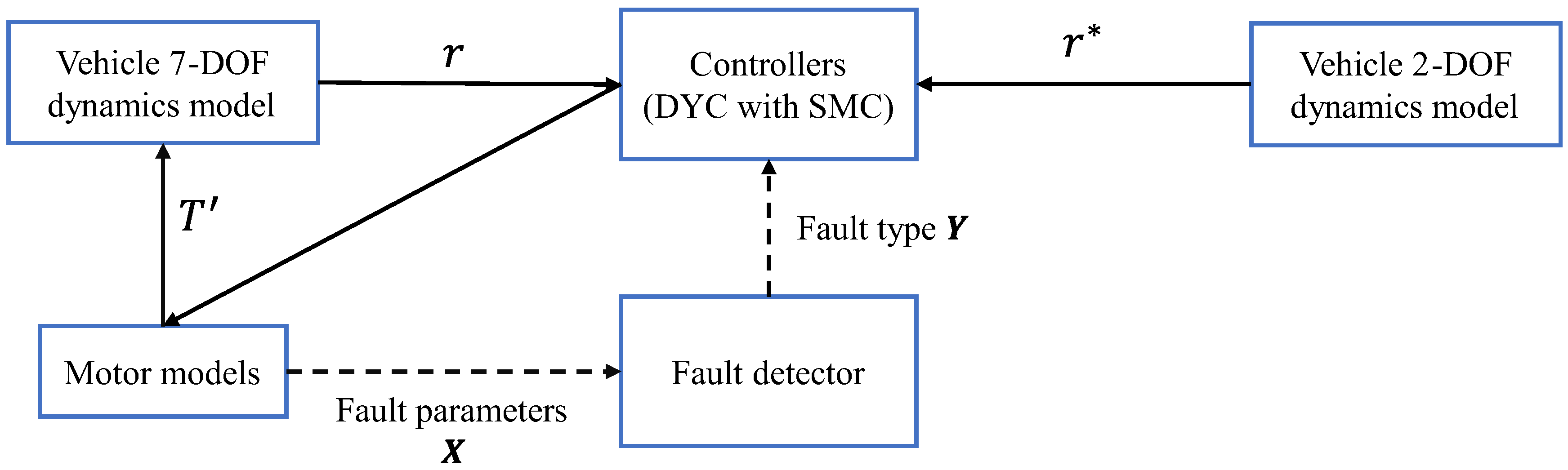
In this research, as shown in Figure 4, the integral system, which combines an BPNN-based motor fault detector and a SMC-based DYC-based fault-tolerant control, is developed. The BPNN-based motor fault detector collects and processes current signals to derive fault parameters , and analyze the motor fault wheel and fault type. According to , to select controllers for different faults, the controller calculates the yaw moment from the desired side yaw rate for the 2-DOF and the feedback yaw rate for the 7-DOF model.
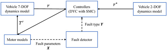
Figure 4.
Schematic diagram of the control system.
3.1. BPNN-Based Motor Fault Diagnosis
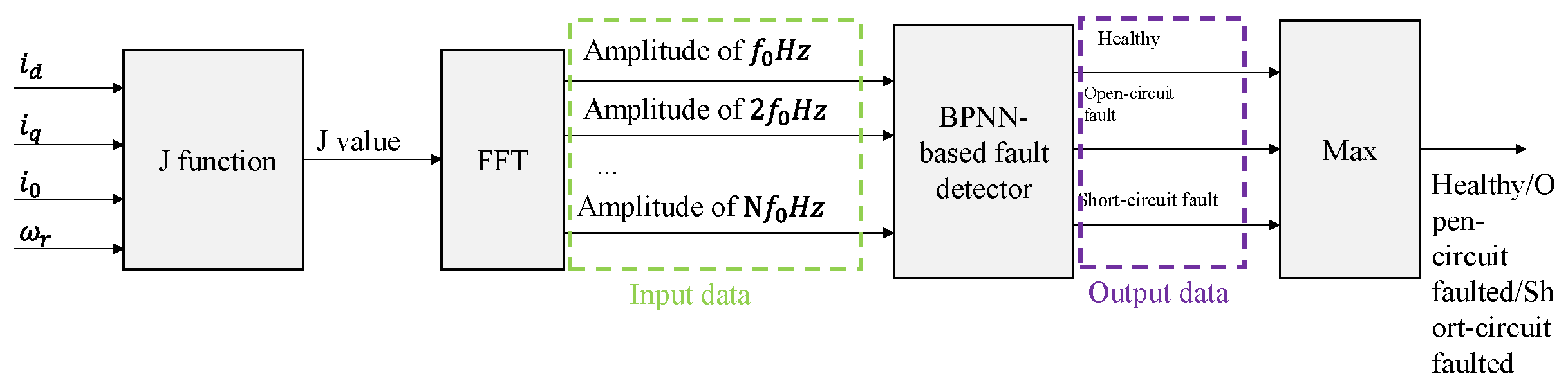
Classical observer-based fault detectors require parameter identification of the motors. It is challenging work, especially for the PMSM. As a result, a model-free BPNN-based motor fault detector is proposed in this research. The flow chart of the proposed BPNN-based motor fault detector is shown in Figure 5.
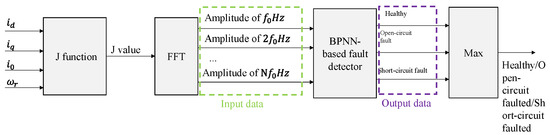
Figure 5.
Flow chat of a BPNN-based motor fault detector.
When a motor fails, its current signals are bound to deviate. In the d-q-0 coordinate system, the current signals are excellent fault indicators.
When no electrical fault occurs in the motor, the training objects are the current of , , and , and at the same time, the angular velocity of the motor rotor needs to be taken into account. So, a fault identification function whose name is “J function” is defined as
Since the function is a time-domain signal, it is difficult to analyze, so the function is transformed into a frequency-domain signal by means of a fast Fourier transform.
For a function with period , the fast Fourier transform is defined as
where the coefficient is
Assuming the reference frequency is , the reference period is .
The fault indicators are the result of Fourier transforms with multiple frequencies of The amplitude of these fault indicators is used to indicate the fault conditions of the motor. In this research, sets of harmonic frequencies are designed and tested.
It is assumed that the motor is categorized into three types of faults: no faults, short circuit faults, and open circuit faults.
The flowchart of the fault diagnosis training structure based on the BP neural network is shown in Figure 6.
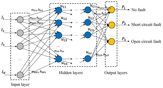
Figure 6.
Schematic diagram of a neural network.
In Figure 6, the are the domain of frequencies of . are random weights of the hidden layers. are the random biases of the neurons. are the neurons in hidden layers. The initial weights and biases are randomly defined at the first step of training. They are updated via the gradient descent method during the training processes.
It is necessary to normalize the input data to the range of . Maximum and minimum normalization methods are used for this step. The normalization process is conducted as follows:
where is the set of the harmonic amplitudes and is defined by
The input layer nodes are amplitudes of different frequencies. The hidden layer may have more than one layer, and the number of nodes in each layer can be defined as desired. The vector of inputs is:
A random weight matrix as well as a bias matrix are defined. Then, the nodes of the first hidden layer are defined as shown as
Hidden nodes need to be activated by the activation function; otherwise, the increase in the number of layers is ineffective. Here, the activation function is chosen as a sigmoid function, shown as
Assuming that the number of hidden nodes is s after hidden layers, the output layer satisfies:
In this study, the output needs to consider the three types of motor faults. So, and the predicted output is defined as
Backpropagation requires adjusting the weight matrix and bias matrix by gradient descent. Define the error as:
Fault labels to be utilized in the training process are defined in Table 1. The state of the motor includes no fault (NF), short circuit fault (SCF), open circuit fault (OCF), and their combinations. The training labels are listed in Table 2.
Table 2.
Definition of fault labels for training.
For layer nodes, the gradient of is obtained by solving the partial derivatives based on the error. It is expressed by
where and are the learning rates. According to the above method, a multilayer neural network based fault recognition indicator can be built.
When the system recognizes the information about the motor fault, it defines the motor torque output coefficient, which means the percentage of the output of the motors. Considering that the recognized motor parameters cannot be exactly integers, a range of parameters is defined whose relationship with the motor fault status coefficients is shown in Table 3.
Table 3.
Fault logic table.
It is quite common that the predicted results do not accurately meet the defined labels. As a result, a function is defined to find the fault state of the motor. The function is defined as
where [.] is the function of rounding down.
3.2. Vehicle Fault Tolerant Control
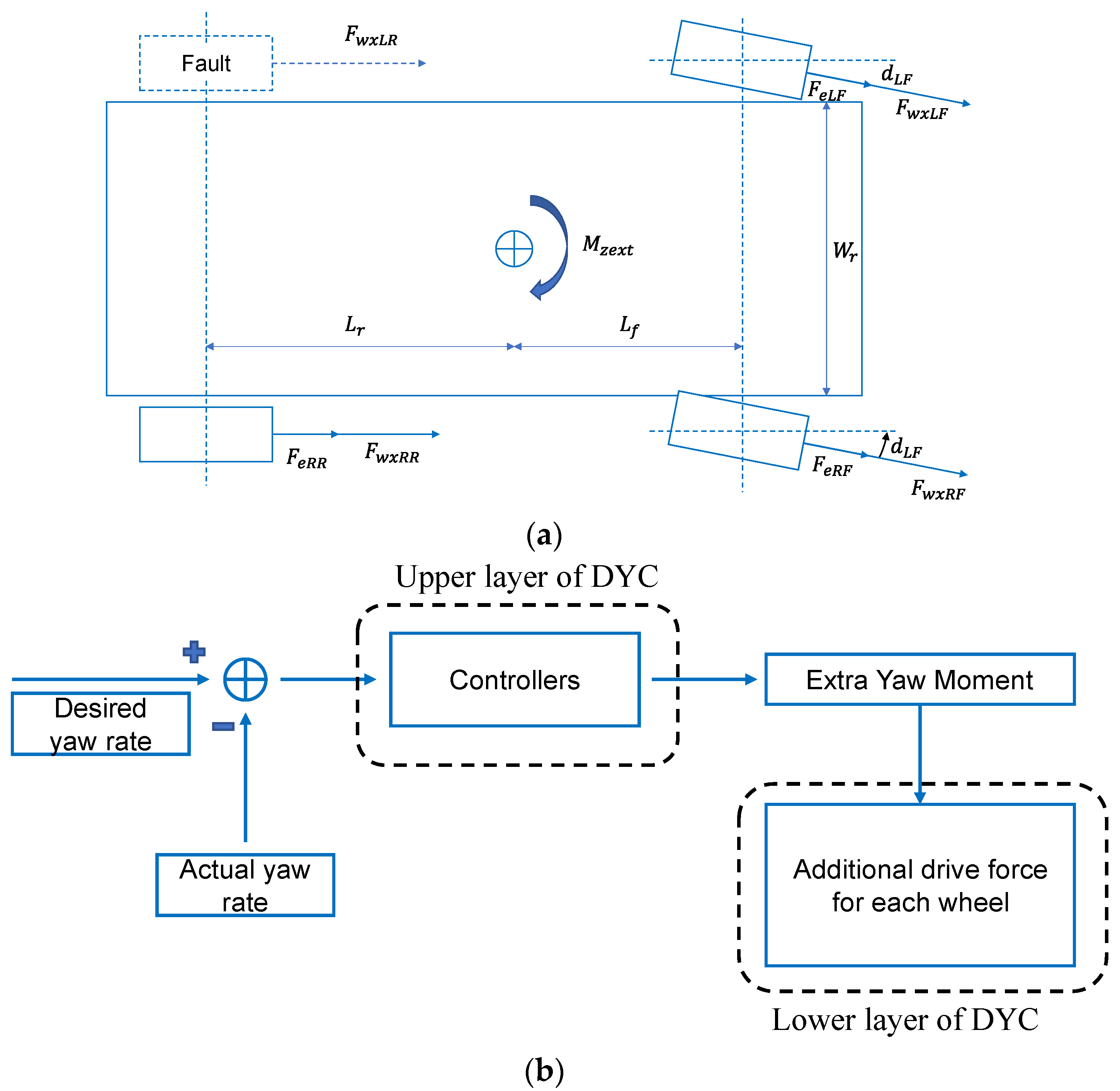
Fault-tolerant control is conducted by a direct yaw moment controller (DYC). In the DYC, there are two layers; SMC is used at the upper level of the controller to calculate the yaw moment. The lower-layer controller distributes proper output torque to each healthy motor to generate the desired yaw moment. Although vehicles with two faulted motors are also possible in fault tolerance, the probability of simultaneous faults of two different wheels is low from practical views. In addition, according to the literature [29], although fault tolerance can be realized for two faulty wheel motors, it is dangerous and not recommended to attempt fault tolerance even when two wheels fail. Therefore, only the case of a one-wheel fault is considered in this study. Figure 7a shows the force analysis of the direct yaw moment control when the left rear motor is faulted, and Figure 7b shows a flowchart of the DYC.
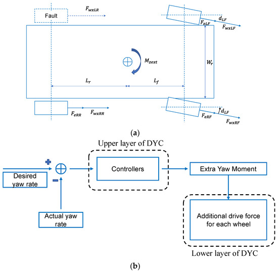
Figure 7.
DYC schematic diagram (a) Force analysis of DYC; (b) DYC flowchart.
3.2.1. Design of the Upper Level of DYC
When DYC is performed, SMC is used for the calculation of the yaw moment.
The equation for the yaw rate is defined as:
Thus, there are
and
A sliding mold surface is defined as
where are the weights of variables and .
The linear reaching law is chosen for the sliding mode, and it is expressed as
where is a constant and .
The function is defined as
Deriving Equation (34) yields
Thus, there is
Simplifying Equation (37) yields
Integrating Equation (38) yields
A stability analysis must be conducted to find the range of the gains. The Lyapunov second law is chosen to complete the analysis.
A function is defined as
If the following two conditions are all met, the system is proven to be stable.
Condition 1: It is always true that and when and only when , .
Condition 2: It is always true that and when and only when , .
Deriving Equation (55) yields
For condition 1, it is obvious that is always true. And only when , . So, condition 1 is met.
For condition 2, when , , and , thus there is
when , , and , thus there is
Therefore, from Equations (55)–(58), there must be . It is also apparent that when and only when , . So, Condition 2 is always met. As a result, the stability of the controller is proven.
3.2.2. Design of the Lower Layer of DYC
The yaw moment calculated by the upper layer is generated by the wheel drive forces. And it is defined as
where , , and are the drive forces from the motors of the left front wheel, right front wheel, left rear wheel, and right rear wheel, respectively. is the desired yaw moment calculated by the DYC. and are the coefficients of the motors which represent the fault conditions of the motors as defined in Table 2.
The driving forces generated by the body need to be 0 to maintain the longitudinal speed of the vehicle and meet the requirements of
Front and rear drive forces are distributed according to the longitudinal distances between the center of gravity and the front and rear axles, which are shown as
The matrix of the extra forces is shown as
Pseudo-reversal is used to obtain extra drive to the wheels.
4. Simulation Experiments
The effectiveness of the proposed system is verified via simulation experiments based on MATLAB/Simulink (version 2022a) due to the high cost and safety risks of road tests. The vehicle models are constructed using the methods proposed in this paper. The parameters of the vehicle are derived from Carsim 8 (Version 8.02). The healthy and faulted motors are constructed via research on PMSMs [30,31].
4.1. Modeling of Three-Phase PMSMs
It is quite dangerous and costly to collect data from realistic-fault PMSMs. And the parameter identification of the PMSMs is also challenging. In this research, models based on MATLAB/Simulink (version 2022a) are constructed for data collection and providing torques to the vehicles.
4.1.1. Model of a Healthy PMSM
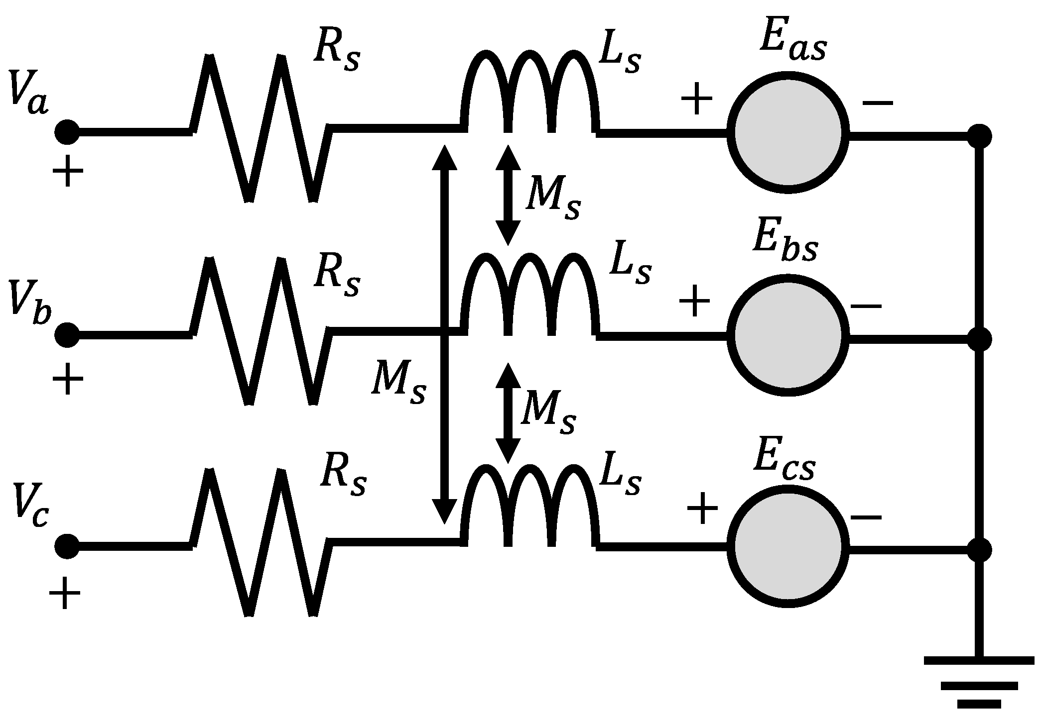
The typical PMSM is represented by an equivalent circuit as shown in Figure 8.
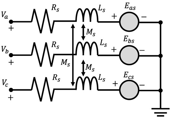
Figure 8.
Schematic diagram of a normal three-phase motor.
The voltage equation is defined as:
where and are the back-electromagnetic forces (back-emf) of three phases, which are defined as
where is the electrical position of the rotor. It has a relationship with the mechanical position of the rotor and is defined as
where is the number of pole pairs of the motor. is the mechanical position of the rotor. is the flux linkage of the permanent magnet of the motor.
The output torque of the motor is defined by
where is the mechanical rotating speed of the motor rotor. It has the relationship between the and is defined as
Park’s transform is often used for motor control. Park’s transform is a method to change the three-phase coordinate of the a-b-c coordinate into another coordinate of d-q-0 for easy control. Park’s transform is described by the transformation matrix which is defined as
For phase currents and voltages, Park’s transform is expressed by
In d-q-0 coordinates, the output torque is expressed as
The desired output torque is represented by: . So, the desired current in q-axis is defined as
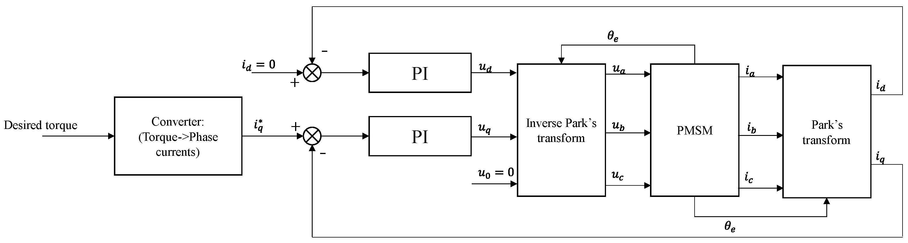
The controller for PMSMs is shown in Figure 9.

Figure 9.
Control diagram of PMSMs.
In Figure 9, represent the voltages transformed by input phase voltages . The controller controls the currents to follow and . proportional-integrational (PI) is used for this controller. The transformed voltages are expressed as
where are the proportional and integral gains of the PI controller, respectively.
The voltages on the d-q axis cannot be expressed directly, so the inverse of Park’s matrix is applied to the controller. The input phase voltages of windings (phase A, phase B, and phase C) are defined by
4.1.2. Modeling a Motor with a Short-Circuit Fault
For a short-circuit fault, the following assumptions are made: (a) The faulted phase is a phase A fault. (b) k percent of the proportional coil is circuited, and the remaining (1 − k) percent turns of the coils work normally. Therefore, the short-circuit is defined as phase f. The equivalent circuit model for a turn-to-turn short circuit fault is shown in Figure 10.
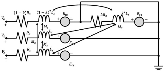
Figure 10.
Equivalent circuit model of a short-circuit fault between turns.
The equivalent motor voltage equation with short-circuit faults is:
where is the resistance of the stator winding of the motor; is the inductance of the stator winding of the motor; is the mutual inductance of the stator winding; and are the input voltage of the three-phase; and are the stator currents of the three phases and the equivalent short-circuited phase, respectively; is the percentage of short-circuited winding turns.
Induced electromotive force and are defined by the flux linkage equation and they are expressed as
The torque equation of the motor with a short-circuit fault is expressed as
4.1.3. Model of Motor with Open-Circuit Fault
Phase A is assumed to be an open-circuit phase, which means phase A is unable to form a closed loop. The equivalent circuit is shown in Figure 11:
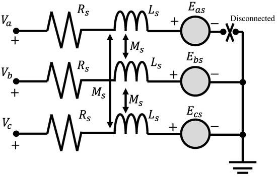
Figure 11.
Equivalent circuit model for an open circuit fault.
The equivalent voltage equation after an open-circuit fault occurs is defined as
The equivalent magnetic chain equation is
The equivalent torque equation is
4.1.4. Motor Demagnetization Fault
The most obvious characteristic of demagnetization faults is the loss of motor torque, which is difficult to model accurately due to the complexity of the demagnetization fault mechanism [9]. Hence, a demagnetization fault is considered a motor shutdown.
4.2. Setting up a Simulation Environment
In order to investigate the effectiveness of the proposed system with the BPNN-based fault detector and the SMC-based DYC-based fault tolerant controller when a single motor fails in a distributed electric vehicle on a wet and slippery road surface, this study selects two typical conditions when the vehicle is driven on highways. The first one is the straight-lane condition, which shows the stability of a vehicle when one motor fails at high speed. The second one is the single-lane change condition at a relatively low speed, which shows the safety of the vehicle for an emergency stop.
All faults are assumed to occur at the left rear wheel. The three main types of faults are turn-to-turn short circuits, open-circuit faults, and demagnetization faults, which are represented by “shutdown”. Motor faults are assumed to occur at . The BPNN-based fault detector is trained offline. The motor parameters used in this study are shown in Table 4. All the parameters of the motor are collected from a real PMSM.
Table 4.
Motor parameters.
The simulation results of the 2-DOF vehicle model are used as references. There are some definitions of simulated vehicles, as listed.
- “2-DOF” represents the reference 2-DOF model.
- “7-DOF” represents the vehicle without any DYC.
- “Open circuit” represents the vehicle with a faulted motor in an open-circuit fault without any DYC.
- “Short circuit” represents the vehicle with a faulted motor of short-circuit fault without any DYC.
- “Shut down” represents the vehicle with a faulted motor and other serious faults without any DYC.
- “Open circuit with SMC” represents the vehicle with a faulted motor in an open-circuit fault with SMC-based DYC.
- “Short circuit with SMC” represents the vehicle with a faulted motor with a short-circuit fault with SMC-based DYC.
- “Shut down with SMC” represents the vehicle with a faulted motor of another fault with SMC-based DYC.
Appropriate noise signals—about 5% of the inputs—are added to the steering angle to better represent the driver’s driving situation in reality.
Vehicle parameters are listed in Table 5. All the parameters of the vehicle are collected from a real passenger car.
Table 5.
Vehicle parameters.
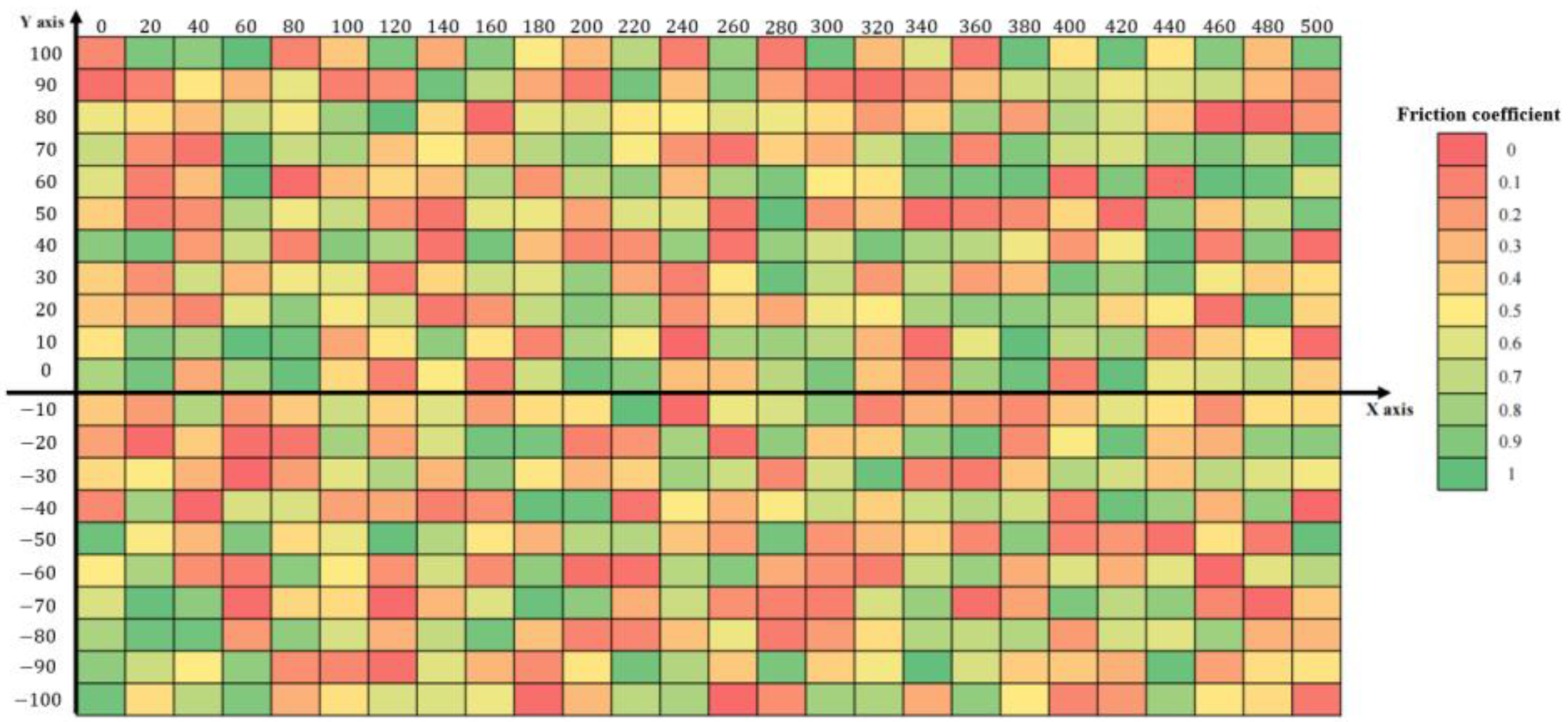
In order to simulate a slippery road surface, an unaveraged road surface friction coefficient is designed [7]. When there is water or ice in the center of the road, the friction coefficient of the road is defined in Figure 12.

Figure 12.
Friction coefficient of the road for simulation tests.
4.3. Motor Fault Diagnosis
The motor fault detector is trained offline. The base frequency of the manually defined function J signal is 0.067 Hz, and the maximum examined frequency is 500 Hz.
The power spectral density in dB is calculated as:
where is the length of data to be analyzed; is the base frequency.
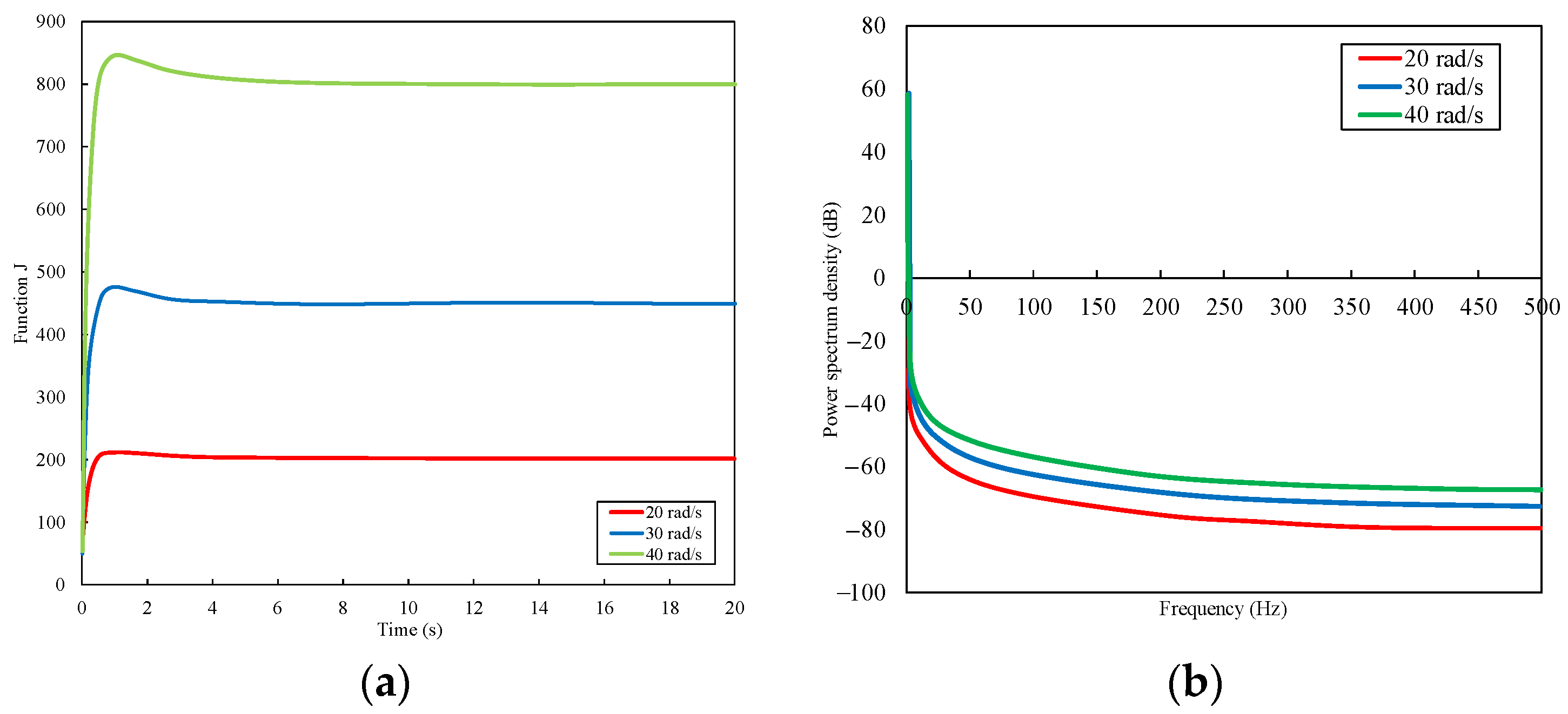
Here is an example of motors with and without faults. For the motors without any fault, the angular speed of the motor was assumed to be constant at 20 rad/s, 30 rad/s, and 40 rad/s, respectively, with a rotational moment of inertia assumed to be and a frictional drag moment coefficient of 0.003 . When the healthy motors operate, the time domain response of the J function and the power spectral density response are shown in Figure 13a,b, respectively.
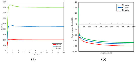
Figure 13.
J functions for normal motors. (a) time domain response; (b) power spectral density response.
From Figure 13, the power spectral densities of healthy motors have the same trend and different amplitudes for different speeds.
The time-domain and power spectral density response of the J-function for the occurrence of short-circuit faults and phase-loss faults is shown in Figure 14a,b.
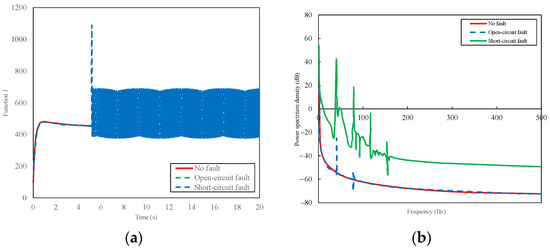
Figure 14.
J functions for normal, open circuit, and short circuit faults. (a) time domain response; (b) power spectral density response.
When the motor is running at a certain speed under fault-free conditions, the J value tends to be stable, and the faster the motor rotates, the higher the power spectral density is, which is shown in Figure 14b. However, when electric faults occur, the J-value will oscillate, and the power spectral density differs from that of healthy motors. Therefore, the power spectral density can be used to determine the state of the fault in motors.
The BPNN is trained based on the simulation of different faulted motors at different speeds. The angular speed is selected as the arbitrary angular velocity from 0 to 130 rad/s. Phase A is assumed to be the fault phase. For short-circuit faults, 35% of the total number of turns are assumed to be short-circuited at the time of the beginning of the fault. In order to better simulate the actual situation, the currents of , , and signal are combined with random white noise. The amplitude of the white noise is 2% of the original signals. The data for this study contains 300 sets, of which 240 are training sets, 45 are validation sets, and 15 are test sets. Meanwhile, the number of fault indication frequency features used for training is 13 (from 0 Hz to 500 Hz, every 38 Hz per feature). After many trials, the number of layers of the neural network is set to 20, and the learning rate is set to 0.001. The hidden neuron nodes are defined as 10 neurons per layer in each hidden layer, and the number of input nodes is set to 13 based on the above frequency analysis.
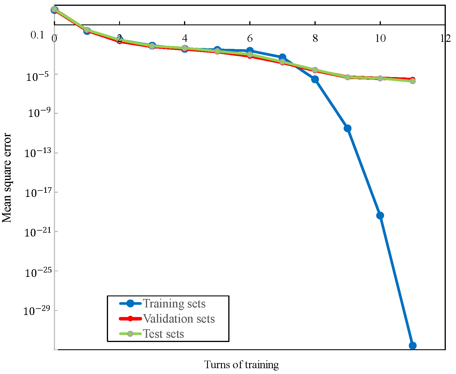
The mean square errors for training sets, verification sets, and test tests are shown in Figure 15.

Figure 15.
Neural network iteration error.
It can be seen that after 10 iterations, the error of the training set reaches the order of , while the error of the test set and the validation set is also at the level of , so the training results can be considered valid.
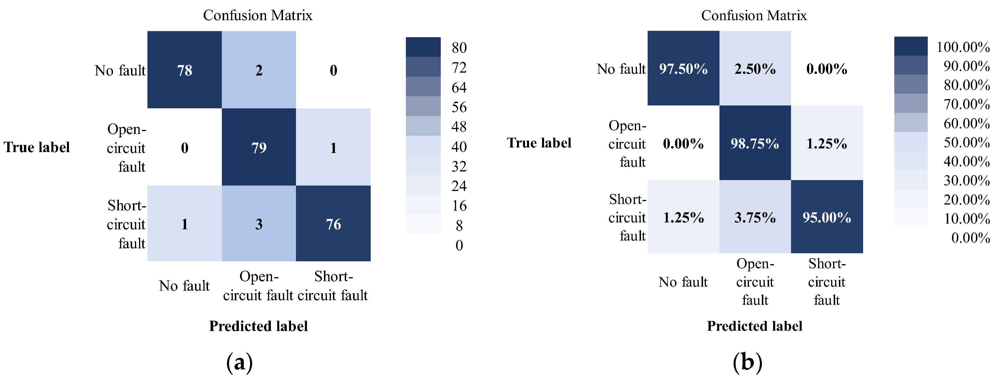
The trained model is input into the whole vehicle model, assuming the vehicle travels in a straight lane at different speeds. A total of 240 sets of tests are further conducted according to different types of faults occurring in different motor positions, and the test results are shown in Figure 16.
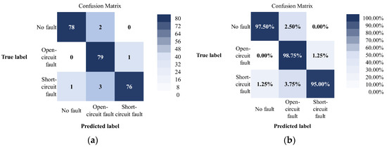
Figure 16.
The confusion matrix of results for BPNN. (a) Confusion matrix of results; (b) Confusion matrix of results in percentage.
In Figure 16a,b, the accuracies of the fault detector in the 240 sets of tests are 97.5% for detecting no fault, 98.75% for detecting open circuit faults, and 95.00% for detecting short circuit faults. The fault detector is accurate and can effectively indicate the type of fault in the motor under vehicle conditions.
4.4. Straight-Lane Condition
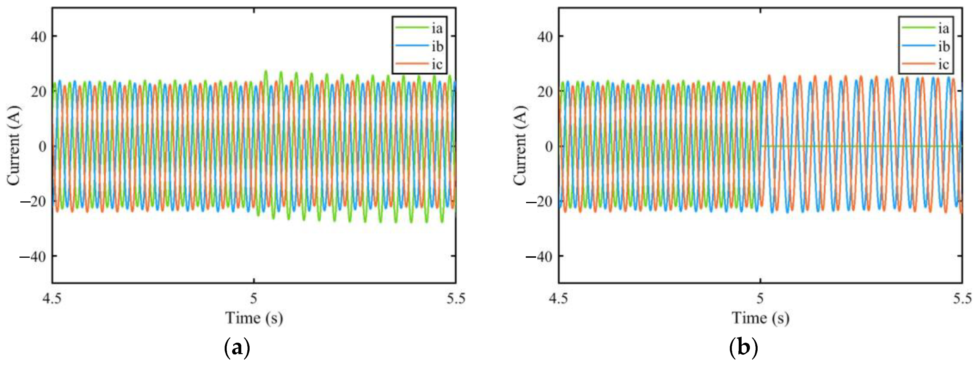
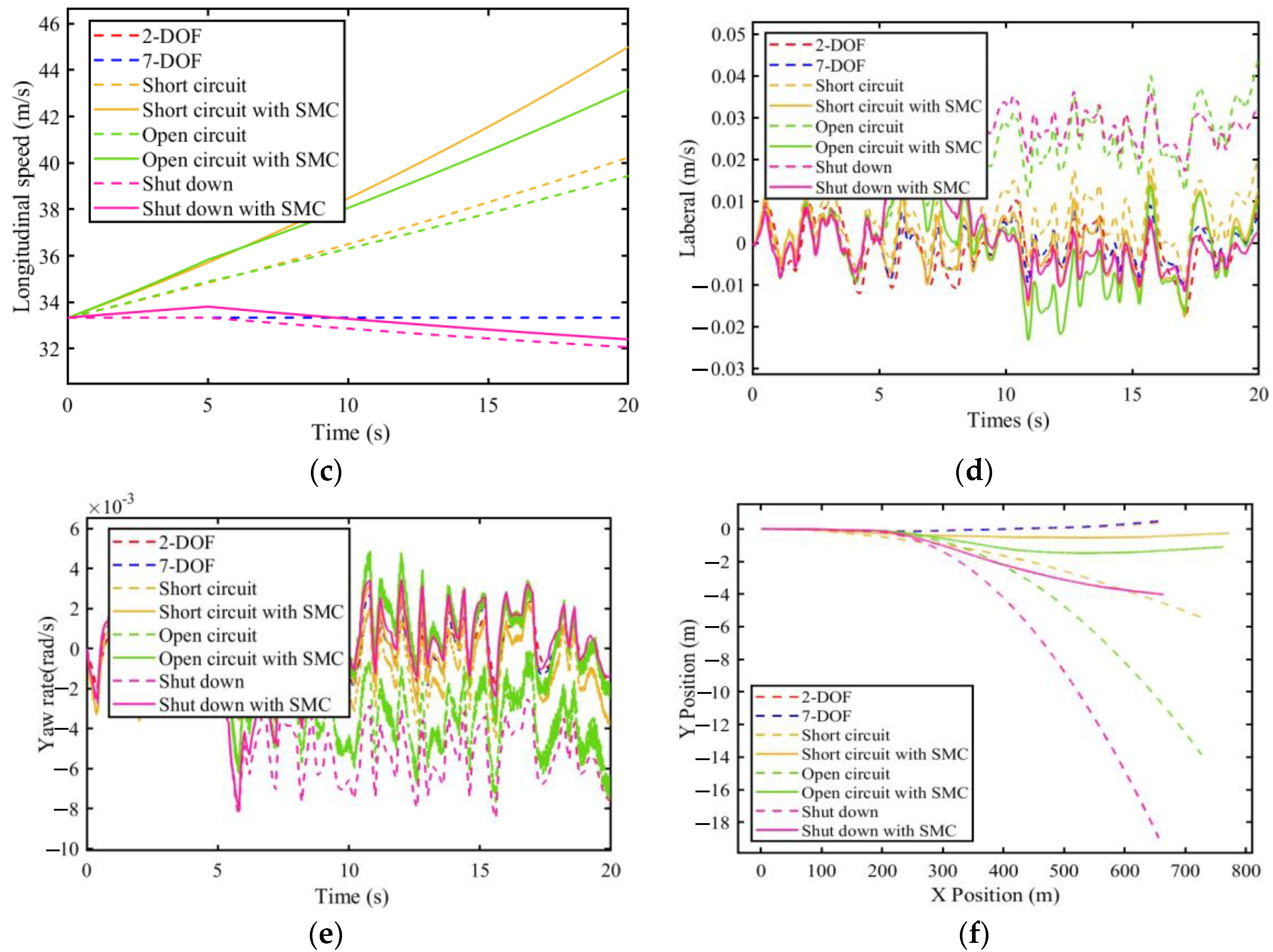
In the 120km/h straight-lane condition, when the left rear motor fails, the phase currents of the motors with short-circuit (SC) faults and open-circuit (OC) faults are shown in Figure 17a,b. Figure 17c–f shows the results of the longitudinal speed, , lateral speed, , yaw rate, and the trajectory of the vehicle, respectively.
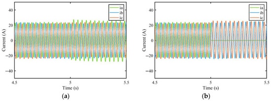
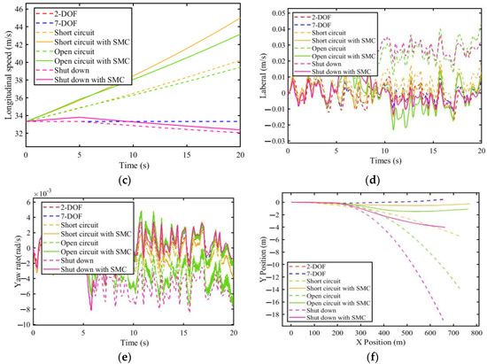
Figure 17.
Simulation results for straight-line driving with a faulted LR motor. (a) Phase currents of the motor with SC faults; (b) Phase currents of the motor with OC faults; (c) Longitudinal speed; (d) Lateral speed; (e) Yaw rate; (f) Trajectory.
The average trajectory offset () and improvement rate ) are also calculated to show the detailed results of the simulation, which are defined by
where represents the average trajectory offset, represents experimental group position, represents control group position (2-DOF), represents total amount of data, represents experimental group improvement rate, and represents faulted experimental group average trajectory offset.
In the straight-lane condition, for the trajectories of the vehicles, only the Y direction is considered.
The s and s are listed in Table 6.
Table 6.
The average trajectory offset and improvement rate for straight-line driving.
The simulation results show that the proposed fault-tolerant controller can effectively control the vehicle with faults and maintain stability on a slippery road. As shown in Figure 17, the trajectories of vehicles with the proposed system are closer to the desired trajectories (trajectories of the 2-DOF model) than those of the vehicles without the proposed system. The system performs best in the event of a short-circuit fault. The improvements of the vehicles with the proposed fault-tolerant controllers compared with the vehicles without them are 77.725%, 73.272%, and 82.201%, respectively, as listed in Table 6. The simulation results show that in straight-lane conditions, the proposed fault tolerant controller is effective under all conditions of motor faults.
4.5. Single Lane Change Condition (SLC)
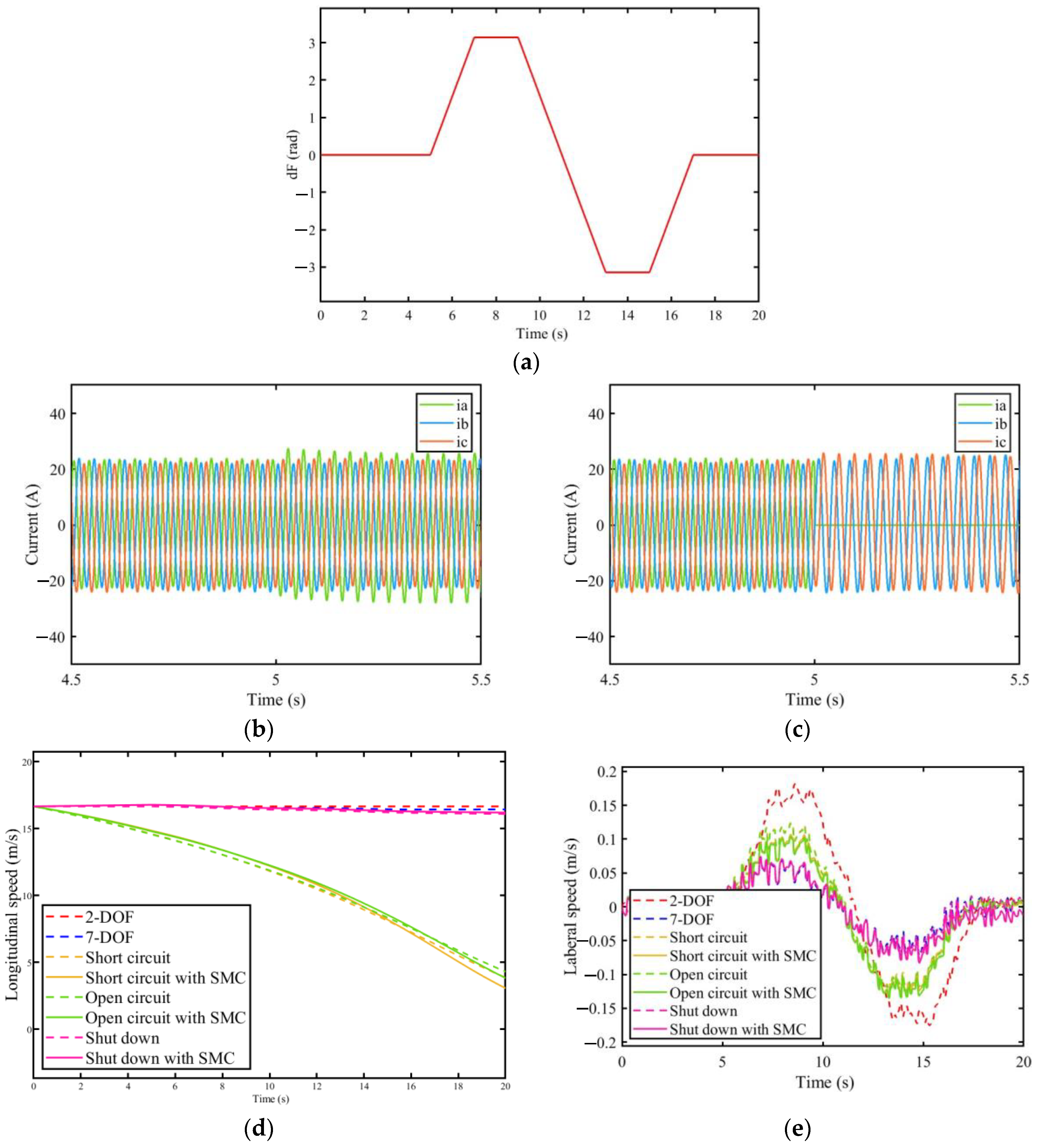
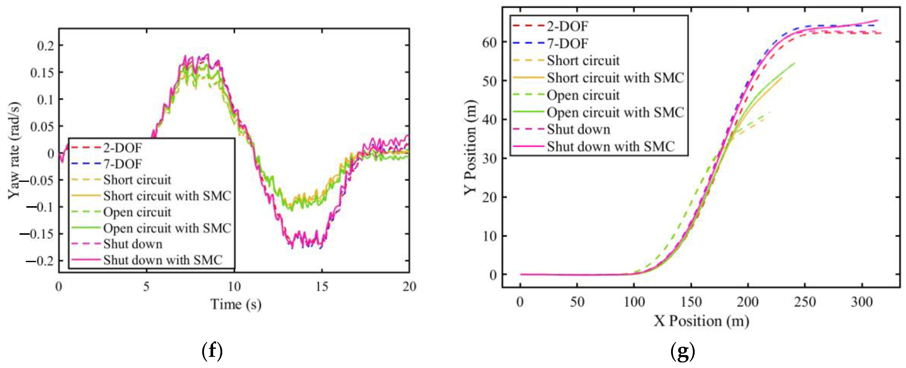
For the single-lane change (SLC) condition, the longitudinal speed is 60 km/h, and the steering angle of the front wheel is shown in Figure 18a. Faults occur at the left rear motor at s. Figure 18b,c show the phase currents of the motors with short-circuit (SC) faults and open-circuit (OC) faults. Figure 18d–g shows the longitudinal speed , lateral speed , yaw rate and the trajectory of the vehicle, respectively.


Figure 18.
Simulation results for SLC with a faulted LR motor. (a) Steering angles of the front wheel; (b) Phase currents of the motor with SC fault; (c) Phase currents of the motor with OC fault; (d) Longitudinal speed; (e) Lateral speed; (f) Yaw rate; (g) Trajectory.
The average trajectory offset (ATO) and improvement rate (IR) are also calculated to show the detailed results of the simulation, which are defined as
where, represents experimental group average trajectory offset, represents experimental group position, represents control group position (2-DOF), represents experimental group position, represents control group position (2-DOF), represents total amount of data, represents experimental group improvement rate, and represents failed experimental group average trajectory offset.
The combined effect of the and directions is considered.
The ATOs and IRs are listed in Table 7.
Table 7.
The average trajectory offset and improvement rate for SLC.
The simulation results show that the proposed fault-tolerant controller can effectively control the vehicle with faults and help steer on a slippery road. As shown in Figure 18, the trajectories of vehicles with the proposed system are closer to the desired trajectories (trajectories of the 2-DOF model) than those of the vehicles without the proposed system. The system performs best in the event of a short-circuit fault. The improvements of the vehicles with the proposed fault-tolerant controllers compared with the vehicles without them are 41.218%, 37.152%, and 44.663%, respectively, as listed in Table 7. The simulation results show that in single-lane change conditions, the proposed fault tolerant controller is effective under all conditions of motor faults.
5. Conclusions
This paper proposes a novel fault-tolerant control system for distributed electric vehicles. It comprises a BPNN-based motor fault detector and an SMC-based, DYC-based fault-tolerant controller. The proposed system demonstrates its remarkable efficacy, particularly in controlling vehicles on slippery road surfaces. Since it works perfectly on simulated slippery road conditions, it is believed that the proposed system can also enhance vehicle safety on real roads, even when the road condition is not good. Specifically, the BPNN-based motor fault detector is precise and reliable in diagnosing fault types and finding the position of faulted motors. Under straight-lane and single-lane change conditions, the DYC-based fault-tolerant controller exhibits notable effectiveness in tolerating motor short-circuit, open-circuit, and demagnetization faults. Simulation results indicate that the vehicles with the proposed system outperform the ones without the proposed system in all faulted motor conditions.
This research not only serves as a comprehensive guide for the practical application of fault detectors and fault-tolerant controllers in distributed electric vehicles but also carries substantial implications for enhancing vehicle safety. Moreover, it contributes significantly to the ongoing development of the electric vehicle industry.
Nevertheless, there are certain limitations to the present study. Firstly, other scenarios and a more extensive range of general working conditions are necessary to enhance the applicability of the system. Secondly, BPNN-based fault detectors have some disadvantages: (a) BPNN requires a large amount of data to achieve high accuracy. It takes more time and requires more samples to obtain a large amount of data on motor faults, which is a challenging task; (b) the computational speed decreases significantly with large data; and (c) the accuracy of BPNN decreases if the dimension of the variables is very large. Lastly, this research uses a simple and constrained friction model between wet and slippery road surfaces and tires, which is common in normal conditions. Some tasks will be required in the future. First, more driving conditions should be tested. Secondly, more data from real motors should be collected and compared with the simulated motors to improve the BPNN-based fault detector. Thirdly, methods to improve the fault detector should be further improved, such as using emerging machine learning approaches, dealing with input data with other signal-proceeding methods, etc. Finally, more road conditions and tire models should also be considered.
Author Contributions
Conceptualization, T.S.; Methodology, T.S. and X.W.; Software, T.S. and X.W.; Investigation, T.S.; Data curation, X.W.; Writing—original draft, T.S.; Writing—review & editing, P.-K.W. and X.W.; Supervision, P.-K.W.; Project administration, P.-K.W. All authors have read and agreed to the published version of the manuscript.
Funding
This research is funded by the research grant of the University of Macau (No. MYRG-GRG2023-00235-FST-UMDF) and Jiangsu Province Science and Technology Special Fund (Innovative Support Project for International Science and Technology Cooperation/ Hong Kong, Macao and Taiwan Science and Technology Cooperation, No. BZ2022055).
Data Availability Statement
Data are contained within the article.
Acknowledgments
The authors thank Hardey Byro for his great support in the writing of this paper.
Conflicts of Interest
The authors declare no conflict of interest.
References
- Gelmanova, Z.S.; Zhabalova, G.G.; Sivyakova, G.A.; Lelikova, O.N.; Onishchenko, O.N.; Smailova, A.A.; Kamarova, S.N. Electric cars. Advantages and disadvantages. J. Phys. Conf. Ser. 2018, 1015, 052029. [Google Scholar] [CrossRef]
- Yao, S.; Bian, Z.; Hasan, M.K.; Ding, R.; Li, S.; Wang, Y.; Song, S. A bibliometric review on electric vehicle (EV) energy efficiency and emission effect research. Environ. Sci. Pollut. Res. 2023, 30, 95172–95196. [Google Scholar] [CrossRef] [PubMed]
- Mariasiu, F.; Kelemen, E.A. Analysis of the Energy Efficiency of a Hybrid Energy Storage System for an Electric Vehicle. Batteries 2023, 9, 419. [Google Scholar] [CrossRef]
- Husain, I.; Ozpineci, B.; Islam, M.S.; Gurpinar, E.; Su, G.J.; Yu, W.; Chowdhury, S.; Xue, L.; Rahman, D.; Sahu, R. Electric Drive Technology Trends, Challenges, and Opportunities for Future Electric Vehicles. Proc. IEEE 2021, 109, 1039–1059. [Google Scholar] [CrossRef]
- Hua, M.; Chen, G.; Zhang, B.; Huang, Y. A hierarchical energy efficiency optimization control strategy for distributed drive electric vehicles. Proc. Inst. Mech. Eng. Part D J. Automob. Eng. 2019, 233, 605–621. [Google Scholar] [CrossRef]
- Liu, Z.; Han, Z.; Zhao, Z.; He, W. Modeling and adaptive control for a spatial flexible spacecraft with unknown actuator failures. Sci. China Inf. Sci. 2021, 64, 152208. [Google Scholar] [CrossRef]
- Salimi, S.; Nassiri, S.; Bayat, A.; Halliday, D. Lateral coefficient of friction for characterizing winter road conditions. Can. J. Civ. Eng. 2016, 43, 73–83. [Google Scholar] [CrossRef]
- Liu, L.; Shi, K.; Yuan, X.; Li, Q. Multiple model-based fault-tolerant control system for distributed drive electric vehicle. J. Braz. Soc. Mech. Sci. Eng. 2019, 41, 531. [Google Scholar] [CrossRef]
- Zheng, J.; Wang, Z.; Wang, D.; Li, Y.; Li, M. Review of fault diagnosis of PMSM drive system in electric vehicles. In Proceedings of the 2017 36th Chinese Control Conference (CCC), Dalian, China, 26–28 July 2017; IEEE: Washington, DC, USA, 2017; pp. 7426–7432. Available online: http://ieeexplore.ieee.org/document/8028529/ (accessed on 23 September 2023).
- Choi, C.; Lee, W. Design and evaluation of voltage measurement-based sectoral diagnosis method for inverter open switch faults of permanent magnet synchronous motor drives. IET Electr. Power Appl. 2012, 6, 526. [Google Scholar] [CrossRef]
- Zheng, P.; Zhao, J.; Liu, R.; Tong, C.; Wu, Q. Magnetic Characteristics Investigation of an Axial-Axial Flux Compound-Structure PMSM Used for HEVs. IEEE Trans. Magn. 2010, 46, 2191–2194. [Google Scholar] [CrossRef]
- Ma, L.; Cheng, C.; Guo, J.; Shi, B.; Ding, S.; Mei, K. Direct yaw-moment control of electric vehicles based on adaptive sliding mode. Math. Biosci. Eng. 2023, 20, 13334–13355. [Google Scholar] [CrossRef] [PubMed]
- Rosero, J.; Romeral, L.; Ortega, J.A.; Urresty, J.C. Demagnetization fault detection by means of Hilbert Huang transform of the stator current decomposition in PMSM. In Proceedings of the 2008 IEEE International Symposium on Industrial Electronics, Cambridge, UK, 30 June–2 July 2008; IEEE: Washington, DC, USA, 2008; pp. 172–177. Available online: http://ieeexplore.ieee.org/document/4677217/ (accessed on 23 September 2023).
- Zhang, L.; Wang, Z.; Ding, X.; Li, S.; Wang, Z. Fault-Tolerant Control for Intelligent Electrified Vehicles Against Front Wheel Steering Angle Sensor Faults During Trajectory Tracking. IEEE Access 2021, 9, 65174–65186. [Google Scholar] [CrossRef]
- Bonci, A.; Indri, M.; Kermenov, R.; Longhi, S.; Nabissi, G. Comparison of PMSMs Motor Current Signature Analysis and Motor Torque Analysis Under Transient Conditions. In Proceedings of the 2021 IEEE 19th International Conference on Industrial Informatics (INDIN), Palma de Mallorca, Spain, 21–23 July 2021; pp. 1–6. [Google Scholar]
- Kao, I.-H.; Wang, W.-J.; Lai, Y.-H.; Perng, J.-W. Analysis of Permanent Magnet Synchronous Motor Fault Diagnosis Based on Learning. IEEE Trans. Instrum. Meas. 2019, 68, 310–324. [Google Scholar] [CrossRef]
- Wang, J.; Fu, P.; Zhang, L.; Gao, R.X.; Zhao, R. Multilevel Information Fusion for Induction Motor Fault Diagnosis. IEEE/ASME Trans. Mechatron. 2019, 24, 2139–2150. [Google Scholar] [CrossRef]
- Guo, G.; Li, P.; Hao, L.-Y. A New Quadratic Spacing Policy and Adaptive Fault-Tolerant Platooning With Actuator Saturation. IEEE Trans. Intell. Transp. Syst. 2022, 23, 1200–1212. [Google Scholar] [CrossRef]
- Deng, H.; Zhao, Y.; Nguyen, A.-T.; Huang, C. Fault-Tolerant Predictive Control with Deep-Reinforcement-Learning-Based Torque Distribution for Four In-Wheel Motor Drive Electric Vehicles. IEEE/ASME Trans. Mechatron. 2023, 28, 668–680. [Google Scholar] [CrossRef]
- Ma, L.; Mei, K.; Ding, S. Direct yaw-moment control design for in-wheel electric vehicle with composite terminal sliding mode. Nonlinear Dyn. 2023, 111, 17141–17156. [Google Scholar] [CrossRef]
- Raksincharoensak, P.; Nagai, M.; Shino, M. Lane keeping control strategy with direct yaw moment control input by considering dynamics of electric vehicle. Veh. Syst. Dyn. 2006, 44, 192–201. [Google Scholar] [CrossRef]
- Peng, H.; Wang, W.; An, Q.; Xiang, C.; Li, L. Path Tracking and Direct Yaw Moment Coordinated Control Based on Robust MPC With the Finite Time Horizon for Autonomous Independent-Drive Vehicles. IEEE Trans. Veh. Technol. 2020, 69, 6053–6066. [Google Scholar] [CrossRef]
- Jin, X.; Yu, Z.; Yin, G.; Wang, J. Improving Vehicle Handling Stability Based on Combined AFS and DYC System via Robust Takagi-Sugeno Fuzzy Control. IEEE Trans. Intell. Transp. Syst. 2018, 19, 2696–2707. [Google Scholar] [CrossRef]
- Yue, Y.; Zhang, R.; Wu, B.; Shao, W. Direct torque control method of PMSM based on fractional order PID controller. In Proceedings of the 2017 6th Data Driven Control and Learning Systems (DDCLS), Chongqing, China, 26–27 May 2017; pp. 411–415. [Google Scholar]
- Komurcugil, H.; Biricik, S.; Bayhan, S.; Zhang, Z. Sliding Mode Control: Overview of Its Applications in Power Converters. IEEE Ind. Electron. Mag. 2021, 15, 40–49. [Google Scholar] [CrossRef]
- Li, X.; Xu, N.; Guo, K.; Huang, Y. An adaptive SMC controller for EVs with four IWMs handling and stability enhancement based on a stability index. Veh. Syst. Dyn. 2021, 59, 1509–1532. [Google Scholar] [CrossRef]
- Venkatesan, M.; Ravi, V.R. Sliding Mode Observer based Sliding Mode Controller for Interacting Nonlinear System. In Proceedings of the Second International Conference on Current Trends in Engineering and Technology (ICCTET 2014), Coimbatore, India, 8 July 2014; pp. 1–6. [Google Scholar]
- Besselink, I.J.M.; Schmeitz, A.J.C.; Pacejka, H.B. An improved Magic Formula/Swift tyre model that can handle inflation pressure changes. Veh. Syst. Dyn. 2010, 48, 337–352. [Google Scholar] [CrossRef]
- Qiu, H.; Qi, Z. A New Motors Fault Tolerance Control Strategy to 4WID Electric Vehicle. In Proceedings of the 2015 6th International Conference on Automation, Robotics and Applications (ICARA), Queenstown, New Zealand, 17–19 February 2015; pp. 17–21. [Google Scholar]
- Mellor, P.H.; Wrobel, R.; Holliday, D. A computationally efficient iron loss model for brushless AC machines that caters for rated flux and field weakened operation. In Proceedings of the 2009 IEEE International Electric Machines & Drives Conference, VOLS 1-3, Miami, FL, USA, 3–6 May 2009; pp. 490–494. [Google Scholar]
- Anderson, P.M. Analysis of Faulted Power Systems; Wiley-IEEE Press: Hoboken, NJ, USA, 1995. [Google Scholar]


Disclaimer/Publisher’s Note: The statements, opinions and data contained in all publications are solely those of the individual author(s) and contributor(s) and not of MDPI and/or the editor(s). MDPI and/or the editor(s) disclaim responsibility for any injury to people or property resulting from any ideas, methods, instructions or products referred to in the content. |
© 2023 by the authors. Licensee MDPI, Basel, Switzerland. This article is an open access article distributed under the terms and conditions of the Creative Commons Attribution (CC BY) license (https://creativecommons.org/licenses/by/4.0/).