
Predictive Model of Adaptive Cruise Control Speed to Enhance Engine Operating Conditions


Abstract
:1. Introduction
2. Predictive Model for EOP
3. Metric for Optimal EOC
3.1. Generic Criteria
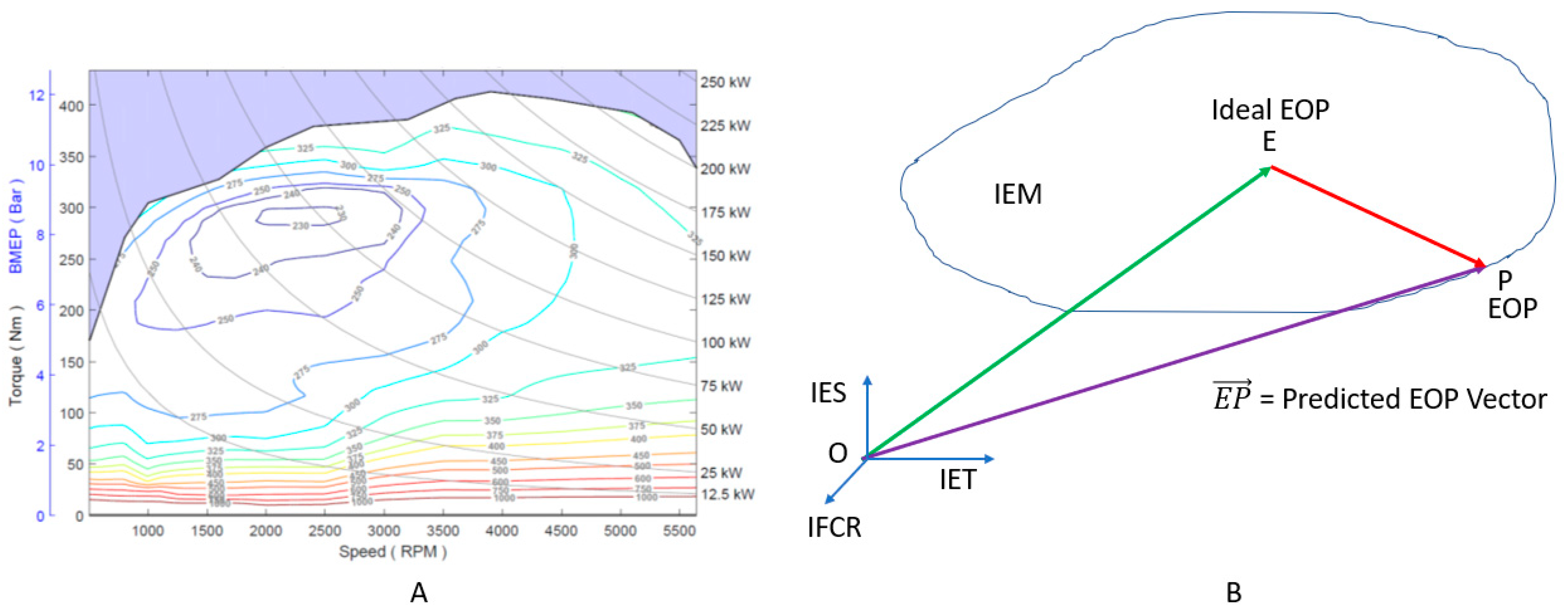
3.2. Euclidean Distance—Ideal EOP
3.3. Engine Caliber—Speed and Torque
3.4. Smoothness Measure—EOC Parameters
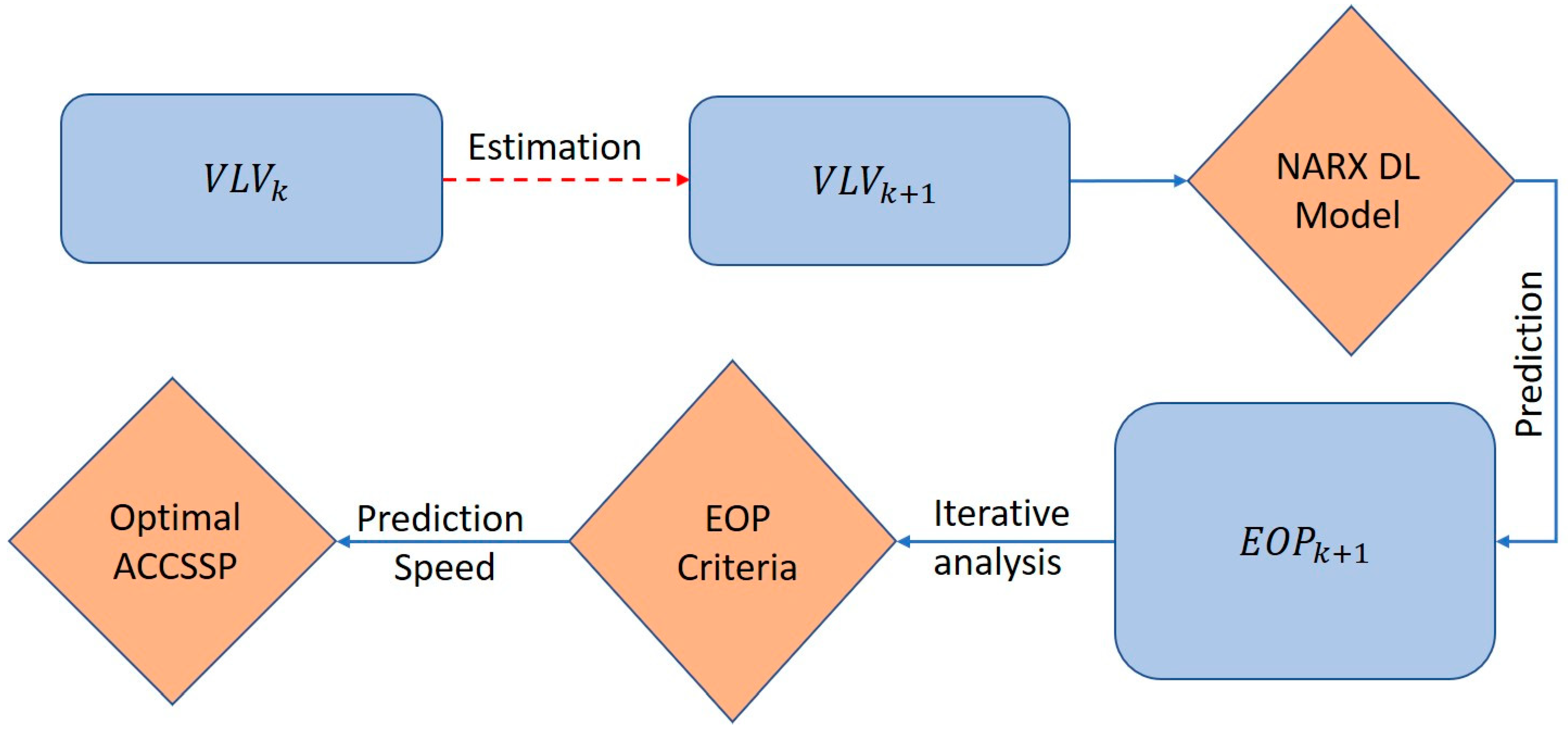
4. Prediction of ACCSSP
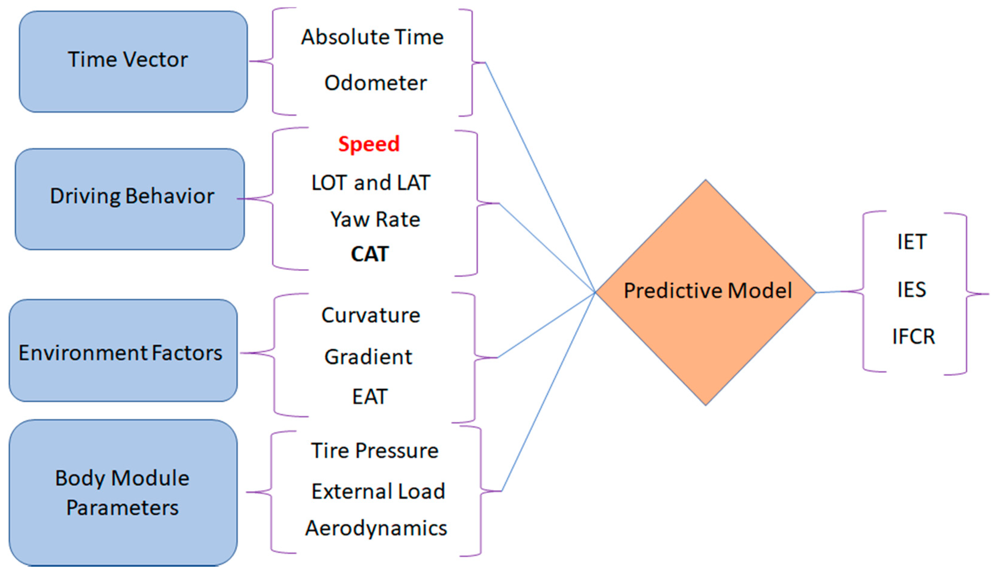
4.1. Estimation of Future Input States—DL Model
4.2. Prediction of Outputs—DL Model
4.3. Estimation of ACC Speed Values—EOC Criteria
4.4. Algorithm to Predict ACCSSP
- Assuming the ACCSSP at is , if the EVS is either +1, , or −1, the highest magnitude among the three is selected as ;
- is chosen closer to (IAS). If this results in two values, then the higher value is considered as ;
- If the eligible speeds at are neither + 1, , nor − 1, then ;
- If for more than 10 s, = + 1 if + 1 SL or − 1 if = SL.
5. Experimental Results
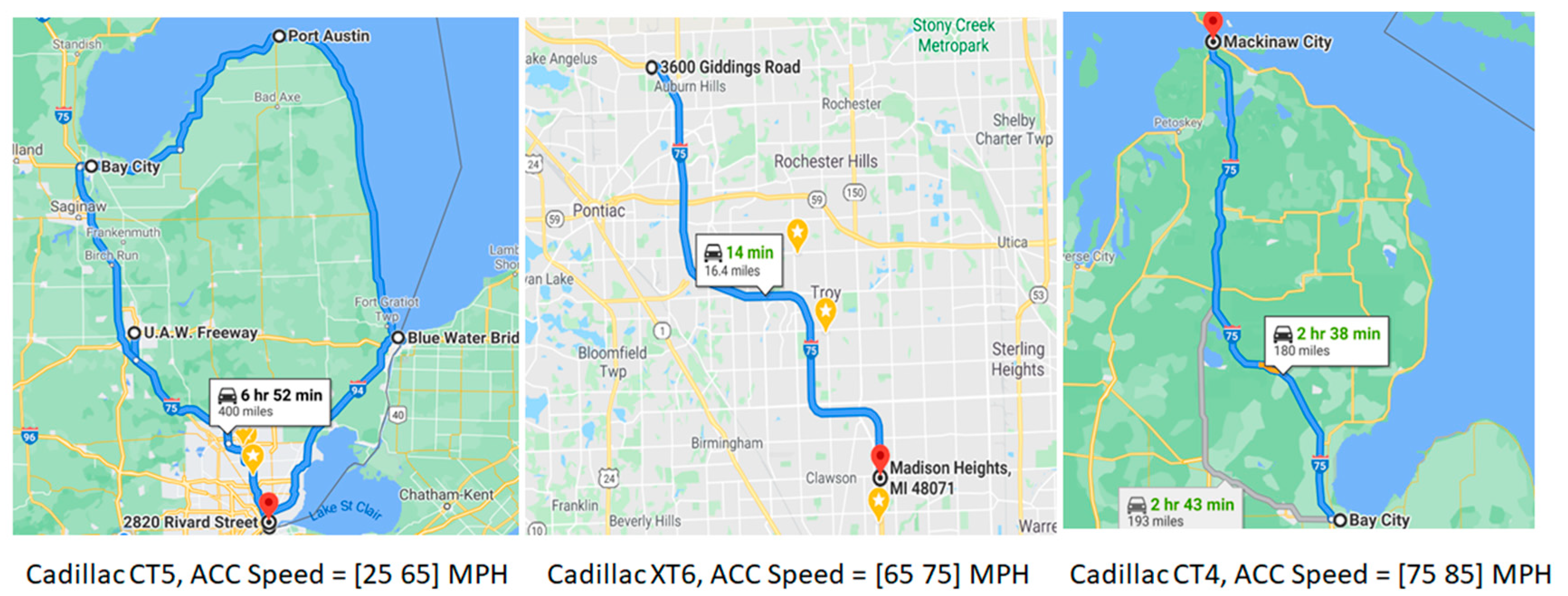
5.1. Dataset Retrieval
5.2. Prediction of EOP
5.3. Estimation of Optimal ACCSSP
6. Discussion
7. Conclusions and Future Work
Supplementary Materials
Author Contributions
Funding
Institutional Review Board Statement
Informed Consent Statement
Data Availability Statement
Acknowledgments
Conflicts of Interest
Abbreviations
| ACC | Adaptive cruise control | |
| ACCSSP | Adaptive cruise control set speed profile (MPH) | |
| Area | Area under the curve | |
| AVS | Allowable vehicle speeds | |
| CAN | Controller area network | |
| CAT | Cabin air temperature (°F) | |
| DL | Deep Learning | |
| DBV | Driver behaviour vector | |
| EAT | External air temperature (°F) | |
| ED | Euclidean distance—Ideal EOP and Predicted EOP | |
| EOC | Engine operating conditions | |
| EOP | Engine operating point | |
| ESC | Engine speed caliber | |
| EVS | Eligible vehicle speeds | |
| ETC | Engine torque caliber | |
| FOD | First order derivative | |
| IAS | Initial ACC speed (MPH) | |
| IEM | Instantaneous engine map | |
| IES | Instantaneous engine speed (rad/s) | |
| IET | Instantaneous engine torque (Nm) | |
| IFCR | Instantaneous fuel consumption rate (1 × 10⁻⁸ ) | |
| ISB | Ideal steering behaviour | |
| LAT | Lateral acceleration (m· ) | |
| LOT | Longitudinal acceleration (m·) | |
| LSTM | Long short-term memory | |
| GMC | General motors corporation | |
| MPH | Miles per hour | |
| MY | Model year | |
| NARX | Autoregressive network with exogenous inputs | |
| OEM | Original equipment manufacturer | |
| RMSE | Root mean square error | |
| RRC | Radius of road curvature (m) | |
| SL | Speed limit (MPH) | |
| SNR | Signal to noise ratio | |
| SSEStdDev | Sum of squared errorsStandard deviation | |
| TP | Tire pressure (kPa) | |
| TPFL | Tire pressure front left (kPa) | |
| TPFR | Tire pressure front right (kPa) | |
| TPRL | Tire pressure rear left (kPa) | |
| TPRR | Tire pressure rear right (kPa) | |
| VLV | Vehicle level vectors | |
| YAR | Yaw rate (rad/s) | |
Nomenclature
| Area of vehicle cross-section () | |
| Aerodynamic drag coefficient | |
| °F | Fahrenheit |
| g | Gravity |
| Hz | Hertz |
| kPa | Kilopascals |
| Kg | Kilogram |
| Km | Kilometres |
| kWh | Kilowatt-hour |
| Lateral acceleration at time step k (m·) | |
| Longitudinal acceleration at time step k (m·) | |
| Mass of the vehicle. (Kg) | |
| Mass of the additional load (Kg) | |
| MPH | Miles per hour |
| m | Meters |
| Meter square (measure of area) | |
| Meter cube per second (volume rate flow) | |
| m. | Meters per second square |
| ms | Milli seconds |
| Nm | Newton meter |
| Rolling coefficient | |
| rad | Radians |
| rad/s | Radians per second |
| Radius of road curvature at time step k (m) | |
| RPM | Rotations per minute |
| Density of air (kg.) | |
| s | Seconds |
| Timestep | |
| Incremental time step (~10 ms) | |
| Gradient of the terrain at time step k (rad) | |
| Yaw rate at time step k (rad/s) | |
| Meter cube per second (Volume rate flow) |
References
- Townsend, J.D.; Calantone, R.J. Evolution and Transformation of Innovation in the Global Automotive Industry. J. Prod. Innov. Manag. 2014, 31, 4–7. [Google Scholar] [CrossRef]
- Katzenbach, A. Automotive. In Concurrent Engineering in the 21st Century; Springer: Cham, Switzerland, 2015; pp. 607–638. [Google Scholar]
- Labuhn, P.I.; Chundrlik, W.J., Jr. Adaptive Cruise Control. U.S. Patent 5,454,442, 3 October 1995. [Google Scholar]
- Marsden, G.; McDonald, M.; Brackstone, M. Towards an understanding of adaptive cruise control. Transp. Res. Part C Emerg. Technol. 2001, 9, 33–51. [Google Scholar] [CrossRef]
- Mahdinia, I.; Arvin, R.; Khattak, A.J.; Ghiasi, A. Safety, Energy, and Emissions Impacts of Adaptive Cruise Control and Cooperative Adaptive Cruise Control. Transp. Res. Rec. J. Transp. Res. Board 2020, 2674, 253–267. [Google Scholar] [CrossRef]
- Stanton, N.A.; Young, M.S. Driver behaviour with adaptive cruise control. Ergonomics 2005, 48, 1294–1313. [Google Scholar] [CrossRef] [Green Version]
- Hoedemaeker, M.; Brookhuis, K. Behavioural adaptation to driving with an adaptive cruise control (ACC). Transp. Res. Part F Traffic Psychol. Behav. 1998, 1, 95–106. [Google Scholar] [CrossRef]
- Kesting, A.; Treiber, M.; Schönhof, M.; Kranke, F.; Helbing, D. Jam-avoiding adaptive cruise control (ACC) and its impact on traffic dynamics. In Traffic and Granular Flow’05; Springer: Berlin, Heidelberg, 2007; pp. 633–643. [Google Scholar]
- Rudin-Brown, C.M.; Parker, H.A. Behavioural adaptation to adaptive cruise control (ACC): Implications for preventive strategies. Transp. Res. Part F Traffic Psychol. Behav. 2004, 7, 59–76. [Google Scholar] [CrossRef]
- Moon, S.; Yi, K. Human driving data-based design of a vehicle adaptive cruise control algorithm. Veh. Syst. Dyn. 2008, 46, 661–690. [Google Scholar] [CrossRef]
- Rosenfeld, A.; Bareket, Z.; Goldman, C.V.; Leblanc, D.J.; Tsimhoni, O. Learning Drivers’ Behavior to Improve Adaptive Cruise Control. J. Intell. Transp. Syst. 2015, 19, 18–31. [Google Scholar] [CrossRef]
- Milanes, V.; Shladover, S.E.; Spring, J.; Nowakowski, C.; Kawazoe, H.; Nakamura, M. Cooperative Adaptive Cruise Control in Real Traffic Situations. IEEE Trans. Intell. Transp. Syst. 2013, 15, 296–305. [Google Scholar] [CrossRef] [Green Version]
- Milanés, V.; Shladover, S.E. Modeling cooperative and autonomous adaptive cruise control dynamic responses using experimental data. Transp. Res. Part C Emerg. Technol. 2014, 48, 285–300. [Google Scholar] [CrossRef] [Green Version]
- Kesting, A.; Treiber, M.; Schönhof, M.; Helbing, D. Adaptive cruise control design for active congestion avoidance. Transp. Res. Part C Emerg. Technol. 2008, 16, 668–683. [Google Scholar] [CrossRef]
- Ploeg, J.; Serrarens, A.F.A.; Heijenk, G.J. Connect & Drive: Design and evaluation of cooperative adaptive cruise control for congestion reduction. J. Mod. Transp. 2011, 19, 207–213. [Google Scholar] [CrossRef] [Green Version]
- Lin, D.-Y.; Hou, B.-J.; Lan, C.-C. A balancing cam mechanism for minimizing the torque fluctuation of engine camshafts. Mech. Mach. Theory 2017, 108, 160–175. [Google Scholar] [CrossRef]
- Lu, C.; Dong, J.; Hu, L. Energy-Efficient Adaptive Cruise Control for Electric Connected and Autonomous Vehicles. IEEE Intell. Transp. Syst. Mag. 2019, 11, 42–55. [Google Scholar] [CrossRef]
- Vedam, N. Terrain-Adaptive Cruise Control: A Human-Like Approach. Ph.D. Thesis, Texan A&M University, Collage Station, TX, USA, 2015. [Google Scholar]
- Kolmanovsky, I.V.; Filev, D.P. Terrain and Traffic Optimized Vehicle Speed Control. IFAC Proc. Vol. 2010, 43, 378–383. [Google Scholar] [CrossRef]
- Gaspar, P.; Németh, B. Design of adaptive cruise control for road vehicles using topographic and traffic information. IFAC Proc. Vol. 2014, 47, 4184–4189. [Google Scholar] [CrossRef] [Green Version]
- Németh, B.; Gáspár, P. Road inclinations in the design of LPV-based adaptive cruise control. IFAC Proc. Vol. 2011, 44, 2202–2207. [Google Scholar] [CrossRef] [Green Version]
- Németh, B.; Gaspar, P. Design of vehicle cruise control using road inclinations. Int. J. Veh. Auton. Syst. 2013, 11, 313. [Google Scholar] [CrossRef] [Green Version]
- Ma, J.; Hu, J.; Leslie, E.; Zhou, F.; Huang, P.; Bared, J. An eco-drive experiment on rolling terrains for fuel consumption optimization with connected automated vehicles. Transp. Res. Part C Emerg. Technol. 2019, 100, 125–141. [Google Scholar] [CrossRef]
- Kolachalama, S.; Lakshmanan, S. Using Deep Learning to Predict the Engine Operating Point in Real-Time; SAE Technical Paper; General Motors LLC: Detroit, MI, USA, 2021. [Google Scholar]
- Diaconescu, E. The use of NARX neural networks to predict chaotic time series. Wseas Trans. Comput. Res. 2008, 3, 182–191. [Google Scholar]
- Kolachalama, S.; Hay, C.L.; Mushtarin, T.; Todd, N.; Heitman, J.; Hermiz, S. An Algorithm to Estimate Steering Behavior Using Vehicle Radius of Curvature; Research Disclosure, Questel Ireland Ltd.: Paris, France, 2018; p. 647068. [Google Scholar]
- Kolachalama, S.; Kuppa, K.; Mattam, D.; Shukla, M. Thermal Analysis of Radiator Core in Heavy Duty Automobile. In Proceedings of the Heat Transfer Summer Conference, Jacksonville, FL, USA, 10–14 August 2008; Volume 48487, pp. 123–127. [Google Scholar]
- Eathakota, V.P.; Kolachalama, S.; Krishna, K.M.; Sanan, S. Optimal posture control for force actuator based articulated suspension vehicle for rough terrain mobility. In Advances in Mobile Robotics; World Scientific: Coimbra, Portugal, 2008; pp. 760–767. [Google Scholar]
- Eathakota, V.; Singh, A.K.; Kolachalama, S.; Madhava Krishna, K. Determination of Optimally Stable Posture for Force Actuator Based Articulated Suspension for Rough Terrain Mobility. In Trends in Intelligent Robotics. FIRA 2010; Communications in Computer and Information Science; Springer: Berlin/Heidelberg, Germany, 2010; Volume 103. [Google Scholar]
- Tanaka, H.; Tokushima, T.; Higashi, H.; Hamada, S. Means for Suppressing Engine Output Torque Fluctuations. U.S. Patent 4,699,097, 13 October 1987. [Google Scholar]
- Li, S.E.; Guo, Q.; Xu, S.; Duan, J.; Li, S.; Li, C.; Su, K. Performance Enhanced Predictive Control for Adaptive Cruise Control System Considering Road Elevation Information. IEEE Trans. Intell. Veh. 2017, 2, 150–160. [Google Scholar] [CrossRef]
- La Valle, S.M. Motion planning. IEEE Robot. Autom. Mag. 2011, 18, 108–118. [Google Scholar] [CrossRef]
- Li, R.; Liu, C.; Luo, F. A design for automotive CAN bus monitoring system. In Proceedings of the 2008 IEEE Vehicle Power and Propulsion Conference, Harbin, China, 3–5 September 2008; pp. 1–5. [Google Scholar]
- Gallardo, F.B. Extraction and Analysis of Car Driving Data via Obd-II. Ph.D. Thesis, Universidad Miguel Hernández de Elche, Alicante, Spain, 2018. [Google Scholar]


| NARX—Deep Learning Model | |||||
|---|---|---|---|---|---|
| Properties | Dataset—Training and Testing | ||||
| Property | Value | Vehicle | Training | Test Size | ACCSSP (MPH) |
| Training function | Levenberg–Marquardt backpropagation | 2020 Cadillac CT5 | 1–14,000 | 14,001–15,000 | 30 |
| Input/Feedback delays | 1:2 | 2020 Cadillac CT5 | 1–24,000 | 24,001–25,000 | 40 |
| Training, Validation | [30,70]% | 2020 Cadillac CT5 | 1–34,000 | 34,001–35,000 | 50 |
| Hidden layer size | 10 | 2020 Cadillac CT5 | 1–44,000 | 44,001–45,000 | 60 |
| Network | Open | 2019 Cadillac XT6 | 1–40,000 | 40,001–41,000 | 70 |
| Performance | MSE | 2021 Cadillac CT4 | 1–25,000 | 25,001–26,000 | 80 |
| Section A | Section B | ||||||||
|---|---|---|---|---|---|---|---|---|---|
| Ideal EOP | Generic | Engine Specific | Smoothness Measure—Spline Fit | ||||||
| Vehicle | IET (Nm) | IES (rad/s) | IFCR | Parameter | Condition | Parameter | Condition | Parameter | Condition |
| Cadillac CT5 | 250 | 140 | 180 | IET | Higher | ED | Lower | Higher | |
| Cadillac XT6 | 280 | 145 | 220 | IES | Higher | ESC | Higher | RMSE | Lower |
| Cadillac CT4 | 240 | 140 | 200 | IFCR | Lower | ETC | Higher | SSE | Lower |
| = 0.013 |
| Time Step | Odometer (Miles) | Speed (MPH) | RRC (m) | YAR (deg/s) | LAT () | LOT () |
| 15,000 | 70 | 8304.140 | 0.216 | 0.117 | 0.437 | |
| 15,000.001 | 70 | 8304.140 | 0.216 | 0.117 | 0.375 | |
| 15,000.003 | 70 | 8304.140 | 0.216 | 0.117 | 0.312 | |
| 15,000.005 | 70 | 9342.157 | 0.192 | 0.104 | −0.125 | |
| 15,000.007 | 70 | 24,912.42 | 0.072 | 0.039 | −0.187 | |
| 15,000.009 | 70 | 74,737.261 | 0.024 | 0.013 | −0.062 | |
| 15,000.011 | 70 | 74,737.261 | 0.024 | 0.013 | 0.25 | |
| 15,000.013 | 70 | 37,368.630 | 0.048 | 0.026 | 0.25 | |
| 15,000.015 | 70 | 24,912.420 | 0.072 | 0.039 | 0.187 | |
| 15,000.017 | 70 | 24,912.420 | 0.072 | 0.039 | 0.187 | |
| 15,000.019 | 70 | 9342.157 | 0.192 | 0.104 | 0.312 |
| EOP | Speed | 65 | 66 | 67 | 68 | 69 | 70 | 71 | 72 | 73 | 74 | 75 |
| IET | Area | 1.6 × 10⁴ | 3.1 × 10⁴ | 4.7 × 10⁴ | 6.2 × 10⁴ | 7.8 × 10⁴ | 9.4 × 10⁴ | 1.1 × 10⁵ | 1.2 × 10⁵ | 1.4 × 10⁵ | 1.6 × 10⁵ | 1.7 × 10⁵ |
| 0.76 | 0.83 | 0.77 | 0.74 | 0.77 | 0.77 | 0.75 | 0.77 | 0.75 | 0.78 | 0.76 | ||
| 0.4 | 0.57 | 0.43 | 0.36 | 0.44 | 0.43 | 0.39 | 0.44 | 0.37 | 0.44 | 0.4 | ||
| SSE | 6.26 | 4.47 | 5.94 | 6.69 | 5.82 | 5.94 | 6.34 | 5.76 | 6.49 | 5.72 | 6.16 | |
| RMS | 0.4 | 0.33 | 0.39 | 0.41 | 0.38 | 0.38 | 0.4 | 0.38 | 0.4 | 0.38 | 0.39 | |
| IES | Area | 1.8 × 10⁴ | 3.5 × 10⁴ | 5.3 × 10⁴ | 7.1 × 10⁴ | 8.9 × 10⁴ | 1.1 × 10⁵ | 1.2 × 10⁵ | 1.4 × 10⁵ | 1.6 × 10⁵ | 1.8 × 10⁵ | 2.0 × 10⁵ |
| 1 | 1 | 1 | 1 | 1 | 1 | 1 | 1 | 1 | 1 | 1 | ||
| 0.99 | 0.99 | 0.99 | 0.99 | 0.99 | 0.99 | 0.99 | 0.99 | 1 | 0.99 | 0.99 | ||
| SSE | 0.003 | 0.002 | 0.003 | 0.003 | 0.003 | 0.003 | 0.002 | 0.001 | 0.001 | 0.001 | 0.001 | |
| RMS | 0.009 | 0.007 | 0.008 | 0.008 | 0.009 | 0.008 | 0.007 | 0.006 | 0.005 | 0.006 | 0.006 | |
| IFCR | Area | 2.8 × 10⁴ | 5.6 × 10⁴ | 8.4 × 10⁴ | 1.1 × 10⁵ | 1.4 × 10⁵ | 1.7 × 10⁵ | 1.9 × 10⁵ | 2.2 × 10⁵ | 2.5 × 10⁵ | 2.7 × 10⁵ | 3.0 × 10⁵ |
| 0.78 | 0.78 | 0.72 | 0.74 | 0.8 | 0.75 | 0.81 | 0.74 | 0.76 | 0.68 | 0.67 | ||
| 0.46 | 0.45 | 0.31 | 0.35 | 0.5 | 0.37 | 0.53 | 0.36 | 0.4 | 0.22 | 0.17 | ||
| SSE | 4913.31 | 4737.99 | 5613.29 | 4967.08 | 3726.95 | 4633.05 | 3429.65 | 4679.59 | 4418.54 | 5766.31 | 6140.52 | |
| RMS | 11.19 | 10.99 | 11.97 | 11.26 | 9.75 | 10.85 | 9.35 | 10.92 | 10.62 | 12.13 | 12.52 | |
| ETC | Area | 5.4 × 101 | 1.1 × 10² | 1.6 × 10² | 2.2 × 10² | 2.8 × 10² | 3.3 × 10² | 3.9 × 10² | 4.5 × 10² | 5.0 × 10² | 5.6 × 10² | 6.2 × 10² |
| 0.788 | 0.781 | 0.724 | 0.739 | 0.802 | 0.751 | 0.814 | 0.745 | 0.759 | 0.689 | 0.671 | ||
| 0.469 | 0.452 | 0.309 | 0.348 | 0.504 | 0.377 | 0.535 | 0.362 | 0.398 | 0.222 | 0.176 | ||
| SSE | 0.02 | 0.02 | 0.025 | 0.023 | 0.017 | 0.022 | 0.016 | 0.023 | 0.022 | 0.03 | 0.033 | |
| RMS | 0.022 | 0.023 | 0.025 | 0.024 | 0.021 | 0.023 | 0.02 | 0.024 | 0.024 | 0.028 | 0.029 | |
| ESC | Area | 1.1 × 10² | 2.2 × 10² | 3.3 × 10² | 4.5 × 10² | 5.6 × 10² | 6.7 × 10² | 7.8 × 10² | 9.0 × 10² | 1.0 × 10³ | 1.1 × 10³ | 1.2 × 10³ |
| 0.822 | 0.869 | 0.824 | 0.801 | 0.826 | 0.817 | 0.799 | 0.812 | 0.783 | 0.807 | 0.792 | ||
| 0.554 | 0.672 | 0.56 | 0.503 | 0.565 | 0.542 | 0.497 | 0.529 | 0.457 | 0.517 | 0.479 | ||
| SSE | 0 | 0 | 0 | 0 | 0 | 0 | 0 | 0 | 0 | 0 | 0 | |
| RMS | 0.003 | 0.002 | 0.003 | 0.003 | 0.003 | 0.003 | 0.003 | 0.003 | 0.003 | 0.003 | 0.003 | |
| ED | Area | 1.9 × 10⁴ | 3.7 × 10⁴ | 5.5 × 10⁴ | 7.2 × 10⁴ | 9.0 × 10⁴ | 1.1 × 10⁵ | 1.2 × 10⁵ | 1.4 × 10⁵ | 1.6 × 10⁵ | 1.7 × 10⁵ | 1.9 × 10⁵ |
| 0.787 | 0.783 | 0.725 | 0.743 | 0.802 | 0.751 | 0.815 | 0.747 | 0.761 | 0.689 | 0.671 | ||
| 0.467 | 0.457 | 0.311 | 0.358 | 0.504 | 0.378 | 0.538 | 0.368 | 0.402 | 0.222 | 0.176 | ||
| SSE | 4896.87 | 4721.42 | 5595.32 | 4950.75 | 3716.68 | 4620.39 | 3421.22 | 4665.06 | 4404.92 | 5749.95 | 6123.26 | |
| RMS | 11.18 | 10.978 | 11.951 | 11.241 | 9.74 | 10.86 | 9.345 | 10.912 | 10.604 | 12.115 | 12.502 |
| Area | SSE | RMS | Area | SSE | RMS | Area | SSE | RMS | ||||||
|---|---|---|---|---|---|---|---|---|---|---|---|---|---|---|
| IE | IES | IFCR | ||||||||||||
| 75 | 69 | 69 | 70 | 70 | 75 | 68 | 68 | 75 | 75 | 65 | 66 | 66 | 75 | 75 |
| 74 | 70 | 70 | 69 | 69 | 74 | 71 | 71 | 71 | 71 | 66 | 69 | 69 | 66 | 66 |
| 73 | 65 | 65 | 71 | 71 | 73 | 70 | 70 | 68 | 68 | 67 | 75 | 75 | 69 | 69 |
| 72 | 68 | 68 | 72 | 72 | 72 | 69 | 69 | 70 | 70 | 68 | 65 | 65 | 65 | 65 |
| 71 | 71 | 71 | 68 | 68 | 71 | 67 | 67 | 72 | 72 | 69 | 70 | 70 | 70 | 70 |
| 70 | 73 | 73 | 73 | 73 | 70 | 72 | 72 | 74 | 74 | 70 | 67 | 67 | 72 | 72 |
| ETC | ESC | ED | ||||||||||||
| 75 | 66 | 66 | 66 | 66 | 75 | 69 | 69 | 70 | 70 | 65 | 66 | 66 | 75 | 75 |
| 74 | 69 | 69 | 65 | 65 | 74 | 70 | 70 | 69 | 69 | 66 | 69 | 69 | 66 | 66 |
| 73 | 75 | 75 | 69 | 69 | 73 | 68 | 68 | 71 | 71 | 67 | 75 | 75 | 69 | 69 |
| 72 | 65 | 65 | 75 | 75 | 72 | 65 | 65 | 72 | 72 | 68 | 65 | 65 | 70 | 70 |
| 71 | 70 | 70 | 70 | 70 | 71 | 71 | 71 | 73 | 73 | 69 | 70 | 70 | 65 | 65 |
| 70 | 67 | 67 | 67 | 67 | 70 | 66 | 66 | 68 | 68 | 70 | 67 | 67 | 72 | 72 |
| 69 | 68 | 66 | 75 | 74 | 67 | 67 | 75 | 67 | 75 |
| 71 | 70 | 65 | 68 | 72 | 71 | 72 | 66 | 75 | 71 |
| 68 | 71 | 67 | 65 | 65 | 74 | 73 | 68 | 73 | 65 |
| Parameters | ACC Speed [25 35] MPH | ACC Speed [35 45] MPH | ||||
|---|---|---|---|---|---|---|
| Inputs | Mean | StdDev | Variance | Mean | StdDev | Variance |
| Absolute time (s) | 2468.020 | 1655.047 | 0.671 | 4584.239 | 2453.828 | 0.535 |
| Odometer (km) | 11,721.440 | 41.765 | 0.004 | 11,596.730 | 56.886 | 0.005 |
| Speed (MPH) | 30.831 | 2.859 | 0.093 | 40.634 | 2.768 | 0.068 |
| ) | 1.090 | 0.652 | 0.598 | 0.808 | 0.449 | 0.556 |
| ) | 0.933 | 0.633 | 0.678 | 0.670 | 0.411 | 0.614 |
| ) | 0.318 | 0.637 | 2.002 | 0.362 | 0.335 | 0.924 |
| YAR (deg/s) | 0.098 | 2.633 | 26.944 | 0.179 | 1.056 | 5.914 |
| EAT (°F) | 12.964 | 0.688 | 0.053 | 14.727 | 1.742 | 0.118 |
| CAT (°F) | 66.141 | 0.348 | 0.005 | 68.895 | 1.069 | 0.016 |
| TPFL (kPa) | 225.908 | 2.915 | 0.013 | 226.990 | 3.243 | 0.014 |
| TPRL (kPa) | 235.773 | 4.640 | 0.020 | 239.900 | 4.259 | 0.018 |
| TPFR (kPa) | 235.115 | 4.834 | 0.021 | 235.575 | 3.706 | 0.016 |
| TPRR (kPa) | 234.132 | 5.742 | 0.025 | 237.544 | 4.270 | 0.018 |
| Outputs | Mean | StdDev | Variance | Mean | StdDev | Variance |
| IET (Nm) | 173.081 | 45.424 | 0.262 | 186.309 | 30.686 | 0.165 |
| IES (rad/s) | 219.483 | 82.421 | 0.376 | 222.809 | 73.464 | 0.330 |
| ) | 380.687 | 204.214 | 0.536 | 378.523 | 139.192 | 0.368 |
| Parameters | ACC Speed [45 55] MPH | ACC Speed [55 65] MPH | ||||
|---|---|---|---|---|---|---|
| Inputs | Mean | StdDev | Variance | Mean | StdDev | Variance |
| Absolute time (s) | 3701.490 | 1808.730 | 0.489 | 2933.845 | 1442.236 | 0.492 |
| Odometer (km) | 11,410.820 | 42.130 | 0.004 | 11,894.840 | 36.372 | 0.003 |
| Speed (MPH) | 51.354 | 2.605 | 0.051 | 60.707 | 2.821 | 0.046 |
| ) | 0.500 | 0.210 | 0.420 | 0.415 | 0.208 | 0.501 |
| ) | 0.336 | 0.208 | 0.619 | 0.257 | 0.214 | 0.835 |
| ) | 0.256 | 0.193 | 0.751 | 0.305 | 0.180 | 0.590 |
| YAR (deg/s) | −0.190 | 0.534 | −2.805 | −0.030 | 0.473 | −15.914 |
| EAT (°F) | 12.889 | 0.556 | 0.043 | 15.083 | 0.670 | 0.044 |
| CAT (°F) | 69.726 | 0.688 | 0.010 | 66.000 | 0.000 | 0.000 |
| TPFL (kPa) | 235.424 | 3.508 | 0.015 | 239.108 | 2.371 | 0.010 |
| TPRL (kPa) | 233.685 | 3.947 | 0.017 | 237.436 | 2.193 | 0.009 |
| TPFR (kPa) | 226.567 | 3.062 | 0.014 | 228.252 | 0.972 | 0.004 |
| TPRR (kPa) | 233.767 | 3.764 | 0.016 | 238.294 | 2.279 | 0.010 |
| Outputs | Mean | StdDev | Variance | Mean | StdDev | Variance |
| IET (Nm) | 234.943 | 25.244 | 0.107 | 254.370 | 27.752 | 0.109 |
| IES (rad/s) | 167.982 | 28.195 | 0.168 | 180.272 | 36.291 | 0.201 |
| ) | 374.715 | 82.660 | 0.221 | 441.351 | 109.691 | 0.249 |
| Parameters | Cadillac XT6, ACC Speed [65 75] MPH | Cadillac CT4, ACC Speed [75 85] MPH | ||||
|---|---|---|---|---|---|---|
| Inputs | Mean | StdDev | Variance | Mean | StdDev | Variance |
| Absolute time (s) | 387.430 | 223.687 | 0.577 | 31.709 | 12.962 | 0.409 |
| Odometer (km) | 12,723.040 | 7.015 | 0.001 | 30,298.330 | 17.042 | 0.001 |
| Speed (MPH) | 70.121 | 1.149 | 0.016 | 77.905 | 1.501 | 0.019 |
| ) | 0.004 | 0.242 | 67.073 | 0.081 | 0.177 | 2.175 |
| ) | −0.091 | 0.188 | −2.079 | 0.108 | 0.189 | 1.748 |
| ) | 0.132 | 0.339 | 2.572 | −0.149 | 0.307 | −2.057 |
| YAR (deg/s) | 0.230 | 0.851 | 3.698 | −0.256 | 0.694 | −2.710 |
| EAT (°F) | 39.225 | 0.296 | 0.008 | 85.039 | 0.998 | 0.012 |
| CAT (°F) | 68.785 | 0.301 | 0.004 | 66.502 | 0.862 | 0.013 |
| Pitch angle (deg) | −0.262 | 0.742 | −2.836 | −0.003 | 0.002 | −0.771 |
| TPFL (kPa) | 241.238 | 2.428 | 0.010 | 227.807 | 0.289 | 0.001 |
| TPRL (kPa) | 235.890 | 0.655 | 0.003 | 249.502 | 0.290 | 0.001 |
| TPFR (kPa) | 243.691 | 1.069 | 0.004 | 228.316 | 0.409 | 0.002 |
| TPRR (kPa) | 235.224 | 1.582 | 0.007 | 249.503 | 0.287 | 0.001 |
| Outputs | Mean | StdDev | Variation | Mean | StdDev | Variance |
| IET (Nm) | 146.803 | 63.428 | 0.432 | 142.117 | 33.698 | 0.237 |
| IES (rad/s) | 183.081 | 7.105 | 0.039 | 205.343 | 17.341 | 0.084 |
| ) | 387.430 | 223.687 | 0.577 | 31.709 | 12.962 | 0.409 |
| EOP | IET | IES | IFCR | ||||||
|---|---|---|---|---|---|---|---|---|---|
| Metric | RMSE | FOD | SNR | RMSE | FOD | SNR | RMSE | FOD | SNR |
| 30 MPH | 2.761 | 1.911 | 35.003 | 2.367 | 1.541 | 35.417 | 12.911 | 8.717 | 25.499 |
| 40 MPH | 0.750 | 0.418 | 45.362 | 0.845 | 0.484 | 37.442 | 14.122 | 9.477 | 24.418 |
| 50 MPH | 1.263 | 0.811 | 45.566 | 1.400 | 0.932 | 43.413 | 18.966 | 13.289 | 25.495 |
| 60 MPH | 0.590 | 0.417 | 51.103 | 0.521 | 0.348 | 51.414 | 21.740 | 15.241 | 25.582 |
| 70 MPH | 0.322 | 0.186 | 53.762 | 0.228 | 0.169 | 58.007 | 8.335 | 5.877 | 30.369 |
| 80 MPH | 0.576 | 0.618 | 46.651 | 0.064 | 0.027 | 70.160 | 9.917 | 6.879 | 27.586 |
| Section: A | Section: B | |||||||||
|---|---|---|---|---|---|---|---|---|---|---|
| Data | IAS = 70 MPH, SL = 75 MPH | Speed (MPH) | Test Cases | |||||||
| Metric | ACCSSP (70 MPH) | ACCSSP (Predicted) | Conformance | SL | IAS | Distance | ED | IFCR | ETC | ESC |
| 35 | 30 | 0.22 | −17.33 | −21.19 | 0.25 | −0.26 | ||||
| Distance | 69,930.00 | 72,028.00 | 934.77 | 45 | 40 | 133.44 | −64.11 | −52.113 | −0.27 | 0.50 |
| ED | 17,4570.83 | 17,4196.86 | −373.96 | 55 | 50 | 712.22 | −366.13 | −323.27 | 0.51 | 1.20 |
| ETC | 572.12 | 573.34 | 1.22 | 65 | 60 | −312.11 | −510.75 | −540.58 | 0.87 | 0.22 |
| ESC | 1154.63 | 1164.83 | 10.20 | 75 | 70 | 934.77 | −373.96 | −379.09 | 1.22 | 10.20 |
| IFCR | 27,4182.80 | 27,3803.70 | −379.09 | 85 | 80 | 801.108 | −1035.28 | −1029.6 | 2.813 | −2.022 |
| EOP | IET | IES | IFCR | ||||||||||
|---|---|---|---|---|---|---|---|---|---|---|---|---|---|
| SL | IAS | SSE | RMS | SSE | RMS | Adj | SSE | RMS | |||||
| 35 | 30 | 0.0 | 0.0 | −9.415 | −0.007 | 0.0 | 0.000 | 0.564 | 0.000 | 0.000 | 0.0 | −103.786 | −0.023 |
| 45 | 40 | 0.0 | 0.0 | 0.326 | 0.001 | 0.0 | 0.000 | 2.582 | 0.013 | 0.000 | 0.0 | −23.251 | −0.005 |
| 55 | 50 | 0.0 | 0.0 | 3.069 | 0.007 | 0.0 | 0.001 | −38.090 | −0.033 | 0.000 | 0.0 | −570.595 | −0.083 |
| 65 | 60 | 0.0 | 0.0 | 1.307 | 0.005 | 0.0 | 0.000 | 0.431 | 0.002 | 0.000 | 0.0 | 33.212 | 0.004 |
| 75 | 70 | 0.0 | 0.0 | 0.368 | 0.004 | 0.064 | 0.160 | −2.607 | −0.024 | 0.000 | 0.0 | 136.612 | 0.044 |
| 85 | 80 | 0.0 | 0.0 | −0.312 | −0.001 | −0.002 | −0.005 | 0.142 | 0.007 | 0.001 | 0.002 | −243.889 | −0.068 |
Publisher’s Note: MDPI stays neutral with regard to jurisdictional claims in published maps and institutional affiliations. |
© 2021 by the authors. Licensee MDPI, Basel, Switzerland. This article is an open access article distributed under the terms and conditions of the Creative Commons Attribution (CC BY) license (https://creativecommons.org/licenses/by/4.0/).
Share and Cite
Kolachalama, S.; Malik, H. Predictive Model of Adaptive Cruise Control Speed to Enhance Engine Operating Conditions. Vehicles 2021, 3, 749-763. https://doi.org/10.3390/vehicles3040044
Kolachalama S, Malik H. Predictive Model of Adaptive Cruise Control Speed to Enhance Engine Operating Conditions. Vehicles. 2021; 3(4):749-763. https://doi.org/10.3390/vehicles3040044
Chicago/Turabian StyleKolachalama, Srikanth, and Hafiz Malik. 2021. "Predictive Model of Adaptive Cruise Control Speed to Enhance Engine Operating Conditions" Vehicles 3, no. 4: 749-763. https://doi.org/10.3390/vehicles3040044
APA StyleKolachalama, S., & Malik, H. (2021). Predictive Model of Adaptive Cruise Control Speed to Enhance Engine Operating Conditions. Vehicles, 3(4), 749-763. https://doi.org/10.3390/vehicles3040044