An Integrated Model for User State Detection of Subjective Discomfort in Autonomous Vehicles

Abstract

The quickly rising development of autonomous vehicle technology and increase of (semi-) autonomous vehicles on the road leads to an increased demand for more sophisticated human–machine-cooperation approaches to improve trust and acceptance of these new systems. In this work, we investigate the feeling of discomfort of human passengers while driving autonomously and the automatic detection of this discomfort with several model approaches, using the combination of different data sources. Based on a driving simulator study, we analyzed the discomfort reports of 50 participants for autonomous inner city driving. We found that perceived discomfort depends on the driving scenario (with discomfort generally peaking in complex situations) and on the passenger (resulting in interindividual differences in reported discomfort extend and duration). Further, we describe three different model approaches on how to predict the passenger discomfort using data from the vehicle’s sensors as well as physiological and behavioral data from the passenger. The model’s precision varies greatly across the approaches, the best approach having a precision of up to 80%. All of our presented model approaches use combinations of linear models and are thus fast, transparent, and safe. Lastly, we analyzed these models using the SHAP method, which enables explaining the models’ discomfort predictions. These explanations are used to infer the importance of our collected features and to create a scenario-based discomfort analysis. Our work demonstrates a novel approach on passenger state modelling with simple, safe, and transparent models and with explainable model predictions, which can be used to adapt the vehicles’ actions to the needs of the passenger.

1. Introduction

Autonomous vehicles (AVs) will have a big impact on our future mobility and society. Users of these vehicles will more often just be passengers instead of drivers, providing them with the freedom to devote their time to other activities, such as reading or relaxing. Despite these advantages, a major point of concern is the perceived loss of control over the vehicle while driving autonomously, which without trust in the vehicle technology, will result in increased levels of discomfort.

Therefore, many researchers are developing methods to prevent this feeling of losing control and thus to increase trust in the technology, through reducing discomfort and improving the individual acceptance of AVs [1]. Most of these methods use the following approaches: (1) Measuring the passenger discomfort and (2) adapting the in-vehicle information presentation and/or driving style of the vehicle to the user’s preferences for discomfort reduction.

A recent work [2] compared seven different studies that investigated comfortable automated driving styles and thereby gave an overview of discomfort-inducing factors in automated driving. The authors stated that the driving dynamics and thus the automated driving style influence perceived driving comfort and discomfort, respectively. To reduce discomfort in automated driving, they concluded that automated driving styles should be designed with a focus on defensive behavior (at least during the system introduction phase) and leave an optional degree of control to the user (e.g., by choosing between different driving styles).

Beggiato, Hartwich, and Krems [3] investigated physiological parameters and their potential to indicate discomfort during automated driving. In a driving simulator, the participants encountered discomfort-inducing approach situations, while physiological parameters such as heart rate and pupil diameter were recorded. The researchers concluded that the investigated physiological parameters could be used to design a real-time discomfort prediction system. A comparable driving simulator study was performed by [4], who recorded heart rate variability and electrodermal activity during driving. Besides manual driving, the participants experienced simulated automated driving with four different automated driving styles. Although, no difference regarding discomfort could be found between the different driving styles, the researchers concluded that electrodermal activity is a promising method to measure discomfort during automated driving. Azevedo-Sa et al. [5] proposed an approach to estimate the trust level in automated driving systems based on state estimation methods. The researchers used a combination of users’ eye tracking signals, usage time of the system, and performance on a non-driving-related task to estimate their trust level. During the study, the participants drove in a driving simulator equipped with a lane keeping assistant, cruise control, and collision avoidance features. The participants could switch between automated and manual driving mode and were allowed to execute a non-driving-related task. Based on questionnaires, the subjective trust, risk, and workload perception for each participant were estimated. In a driving simulator study with 20 participants, Dommel, Pichler, and Beggiato [6] evaluated two mathematical models to predict discomfort perceived during automated approach situations. Using a handset control, participants were able to indicate perceived discomfort in real-time while their heart rate, blink rate, and pupil dilation were recorded. The authors used z-scores of these physiological features to predict the participants’ discomfort. One model was fitted for each of the 20 participants. The researchers found that the tested models performed similarly in terms of mean prediction accuracy, which was around 72%. It was hypothesized that the models’ performances could be further increased by including more discomfort-related input features such as facial expressions or body movements. Trende et al. [7] demonstrated how the discomfort prediction for overtaking maneuvers can be improved by combining contextual, physiological, and user-specific data. Based on data recorded in a driving simulator study [8], the researchers worked on predicting users’ discomfort indicated via handset control during automated driving. Deep neural networks were trained on different sets of input features. The simplest model just used contextual and behavioral information of the automated vehicle such as velocity, lateral acceleration, or time-headway. Heart rate and related features were added for the evaluation of a second model. Although this work showed moderately good model performances, the models were only trained on discomfort inducing parts of the data (where overtaking was performed) and the explainability and reliability of the used deep neural networks is limited.

In this work, we build upon the results of Trende et al. [7] and expand it with two novel approaches. We investigate different methods to use simple and easily explainable models, which are robust and safe, and we use the SHAP (SHapley Additive exPlanations) method [9] to explain how these models operate. Using such a transparent and explainable setting allows us to infer the importance of specific features, including sensory measures, for instance heart rate and eye gaze, and enables the usage of this information for later adaptions of the in-vehicle information presentation and automated driving style.

This work is divided as follows: In Section 2, the conducted study is explained, together with the data pre-processing, how we split data into contexts, and a summary on how the SHAP method works. In Section 3, the results are discussed, followed by the conclusions of this work in Section 5.

2. Materials and Methods

2.1. Data Acquisition

For data acquisition, we conducted a driving simulator study with 50 participants (28 female, 22 male). The sample had a mean (M) age of 25.9 years (standard deviation (SD) = 4.7) and consisted of car drivers with a valid driver’s license, but without prior experience with autonomous driving. After an extensive explanation of the experimental procedure, all participants gave written informed consent prior to study conduct. Upon study completion, they received a monetary compensation.

All participants experienced two simulated autonomous rides: a short familiarization ride and a diversified test ride along a 7 km long, mainly urban, test track. The test track included sections with low traffic density, which only required driving straight ahead, as well as complex scenarios with high traffic density, which required additional driving maneuvers. These complex scenarios included two lane changes to the oncoming lane to bypass obstacles on the own lane as well as two approaches to traffic-light controlled intersections based on a Green Light Optimized Speed Advisory (GLOSA) system, which could result in seemingly unintuitive (yet safe) maneuvers (e.g., approaching a red traffic light without braking, since it would turn green at the time of arrival). The data presented in this paper originate from the test ride. Both rides took place in a fixed-base driving simulator (see Figure 1), which consisted of a fully equipped vehicle interior, a projector-based 180° horizontal field of view extended by a rear-view mirror and two side mirrors, and the SILAB 5.1 simulation environment. Participants experienced both rides from the passenger seat of the driving simulator in order to gain a more realistic impression of autonomous driving.

For the real-time assessment of discomfort during driving, we applied a manual input device for continuous self-report, which served as ground truth for data modelling, as well as a sensor set-up, which gathered potential discomfort features (see Figure 1). The manual input device was a professional handset control (ACD pro 10) with a corresponding continuous response scale ranging from 0 (comfortable) to 100 (uncomfortable) (see [10] for details on this method). During driving, participants pressed the lever of the handset control depending on the extent of their currently perceived discomfort. Stronger pressing of the lever, which lead to higher values on the response scale, indicated higher discomfort. Participants practiced using the handset control during the familiarization drive. The sensor set-up included the driving simulator for parameters of the driving environment and the autonomous driving behavior, a Microsoft Band 2 for physiological parameters (Blood volume pulse, BVP) and the SMI Eye Tracking Glasses 2 for gaze parameters and pupil dilation data.

Driving simulator data including handset control data was recorded with a frequency of 60 Hz. Using independent data loggers each, MS Band 2 data was recorded with a frequency of 10 Hz and eye tracking data was recorded with a frequency of 60 Hz. All data loggers were continuously synchronized during a study conduct based on the network time protocol. After recording, we synchronized all sensor data in a PostgreSQL data storage and analysis framework (see [11] for details) by adding the data of all sensors to the corresponding timestamps of the driving simulator data.

After data processing, the data set consists of 745,931 samples, each with 26 contextual features (CF) and 8 passenger state features (PF). The CF contain vehicle sensor measurements, for example the velocity and lane position of the ego vehicle (the vehicle the participant sits in) and the distances and velocities of other vehicles in the vicinity of the ego vehicle. The PF contain the before-mentioned eye gaze and heart rate data and the respective processed data, which will be covered in the following chapter.

2.2. Passenger Data Processing

Processing of BVP data: The MSBand 2 automatically provides the interval between two successive pulses at every pulse (interbeat interval, IBI), which we used for calculating features regarding heart rate and heart rate variability. In order to reduce the number of artefacts in the data, all IBI values below 400 or above 1500 ms were removed from the data. In addition, IBI values were removed if the jump of the heart rate calculated from the IBI between two successive beats is greater than corresponding to 30 beats per minute [12,13]. From the cleaned IBI time series, we then calculated the heart rate mean, SD, and slope in rolling windows of 10 s. In addition, as indicator for the heart rate variability (HRV), the root mean square of successive differences (RMSSD) between the IBIs (e.g., see [14]) was calculated for windows of 10 s length.

Processing of eye tracking data: The eye tracker provides raw pupil diameter values for the left and right eye. As recommended in the literature, pupil data were preprocessed including removal of implausible values (below 1.5 mm and above 9 mm), elimination of dilation speed artefacts, and trendline deviation outliers [15]. The data for both eyes was averaged to obtain one data stream for pupil dilation. Mean and standard deviation of pupil diameter data were calculated for windows of 10 s length. In addition, SD of gaze vector in x, y, and z components were calculated for the same window length.

2.3. Contextual Data Clustering

A vehicle always drives within a certain traffic context, i.e., a collection of environmental features that are measured and processed by the vehicle. In this work, we will further refer to this traffic context simply as context. The context is important for discomfort prediction, since there are certain contexts that will more likely result in high discomfort, e.g., overtaking. When driving autonomously, we assume the vehicle knows the context it is into a certain degree. For example, the context “overtaking” should be known to the vehicle, since it is the actor that initiated the maneuver. Other works (e.g., [16,17]) also discussed clustering approaches that could be used to derive meaningful contexts with regards to discomfort. Therefore, we assume that such time series data collected by the autonomous vehicle can be split into contexts.

Every context has some unique properties within its sensory time series data, which separate this context from others. For example, all overtaking maneuvers consist of a lane change, high relative speeds, and some obstacle that is overtaken. These factors are recorded by sensors and give a certain “fingerprint” to a context. Training a regression model for each clustered context to classify the discomfort of the passenger has the following advantages: each model has to explain fewer complex relationships between context and discomfort, which increases performance and also makes model explanation methods more precise and applicable. This clustering of data into contexts allows to create a so-called ‘mixture of experts’ (MoE), popularized by Jacobs et al. [18]. The idea is to create multiple simple models that only operate within a certain contextual scope.

In this work, we considered two of those scopes, the overtaking maneuver and the GLOSA scenario. For one of our model approaches (all approaches are covered in Section 3.2), we split the data into three parts. The first part only contained observations from when an overtaking maneuver occurs, the second part contained observations from GLOSA scenarios and the third part the rest of the data. This way and using the ‘mixture of experts’ approach from Jacobs at al., we trained situation-specific models on the overtaking and GLOSA data. Additionally, we used the SHAP method on these models to analyze the specific model explanations.

2.4. Data Modelling and SHAP Method

Every time-step of the recorded data serves as a single observation, which is the input for our prediction model. The handset control value is the prediction target $y_i$ for each observation i. The recorded data was split into test and train sets by randomly splitting observations with 70% being in the train set and 30% in the test set.

For prediction, we used linear models with L2 regularization (Ridge regression), because they are fast and easy to interpret. We believe that simple models like linear models are capable of the prediction task, because humans will likely not classify a situation as uncomfortable after calculating complex, non-linear feature relations, but by applying simple heuristics and relations considering their environment. The model output is the predicted discomfort $y_i^{’}$ for each observation i.

To determine our model performance, we used the coefficient of determination $R^2$. It is defined as

$$R^2=1-u/q,$$

with u being the residual sum of squares

$$u={\displaystyle \sum }_i{\left(y_i-y_i^{’}\right)}^2$$

and q being the total sum of squares with $\widehat{y}$ being the mean of y

$$q={\displaystyle \sum }_i{\left(y_i-\widehat{y}\right)}^2.$$

$R^2$ will be 0 for a baseline model that only predicts the mean of the observed data, negative if a model is worse than the baseline model, and 1 if the model perfectly predicts the target data.

One of the previously mentioned explanation methods is the SHAP (SHapley Additive exPlanations) method by Scott Lundberg [9]. This method calculates an importance measure for each input feature and prediction made by the prediction model. These measures originate from the game theoretic approach of credit assignment and thus can be interpreted as an explanation of the prediction. In the SHAP approach, each model always has an expected output over the data set. For each observation, every feature $f_n$ has a certain impact on the model output that moves the output away from the expected value. An illustration is shown in Figure 2 (top). These impacts are called SHAP values and every feature has a SHAP value for every prediction made by the model and is therefore called local. The impact of features over multiple predictions is often displayed as a SHAP summary plot (Figure 2, bottom), where one point represents the local SHAP value for a single prediction (x-axis) and the color gives additional information over the feature value, allowing to interpret correlations between feature distribution and feature impact. Averaging the absolute SHAP values of one feature over all predictions gives a global feature importance, where the feature with the highest value is the most impactful in the model. This rating is also used as the ranking in the SHAP summary plot, with the topmost feature being the most important overall.

The calculation of the SHAP values is very complex and would exceed the scope of this paper. Simplified, the SHAP method compares the output of a given model and input vector with feature $f_n$ present and with $f_n$ missing. The change of the output with $f_n$ missing is a measure about the importance and the direction of influence of the feature to the model. This is applied for all features in different combinations to remove inter-feature correlations. SHAP values also contain important game theoretic ground truths, defined by Lloyd S. Shapley, that guarantee an exact calculation of these feature importances. For a deeper explanation we recommend to read the work from S. Lundberg [9].

The locality of the SHAP model has the important advantage that specific situations can be explained, e.g., SHAP values of a single overtaking maneuver can be used to explain why a passenger felt uncomfortable in exactly this maneuver. We will use this method to analyze the features’ impacts on the passenger’s discomfort for different model approaches.

3. Results

3.1. Handset Control Data

For an overview of the discomfort experienced by passengers during the autonomous test ride, Figure 3 displays handset control data of all 50 participants along the course of the test track.

The pattern of this data illustrates two characteristics of passengers’ discomfort experience in autonomous driving. First, perceived discomfort depends on the driving scenario. Thus, handset control data of most participants clearly peak at the same points along the test track. All of these shared peaks occur during complex scenarios, such as obstacles on the road or intersections. These scenarios are characterized by high traffic density and the necessity for driving maneuvers in close proximity to other road users, such as changing lanes or braking in convoy in front of a red traffic light. In contrast, only very low discomfort values indicated by only few participants are observable for less complex scenarios with low traffic density and no necessity of driving maneuvers other than driving straight ahead. Therefore, complex driving scenarios contain a comparably high likelihood of passenger discomfort in autonomous driving (cf. [19,20]). Second, perceived discomfort differs between individuals. Thus, the handset control values of the individual participants scatter visibly around the shared basic pattern. These interindividual differences relate to the driving scenario (i.e., which situations are perceived as uncomfortable?), the beginning and end of the discomfort experience (i.e., how long before approaching/after leaving such a situation does discomfort emerge/remain?), and the extent of discomfort (i.e.,: How uncomfortable was the situation?). It is likely that these individual differences in experiencing discomfort during autonomous driving can be attributed to passenger characteristics such as system experience, driving experience, or personality factors (cf. [2]). In summary, these results strongly suggest that modelling approaches need to include data of the driving context as well as passenger-related data that allow to distinguish between different passengers (e.g., physiological and behavioral parameters) for a reliable real-time detection of individual passengers’ discomfort during autonomous driving.

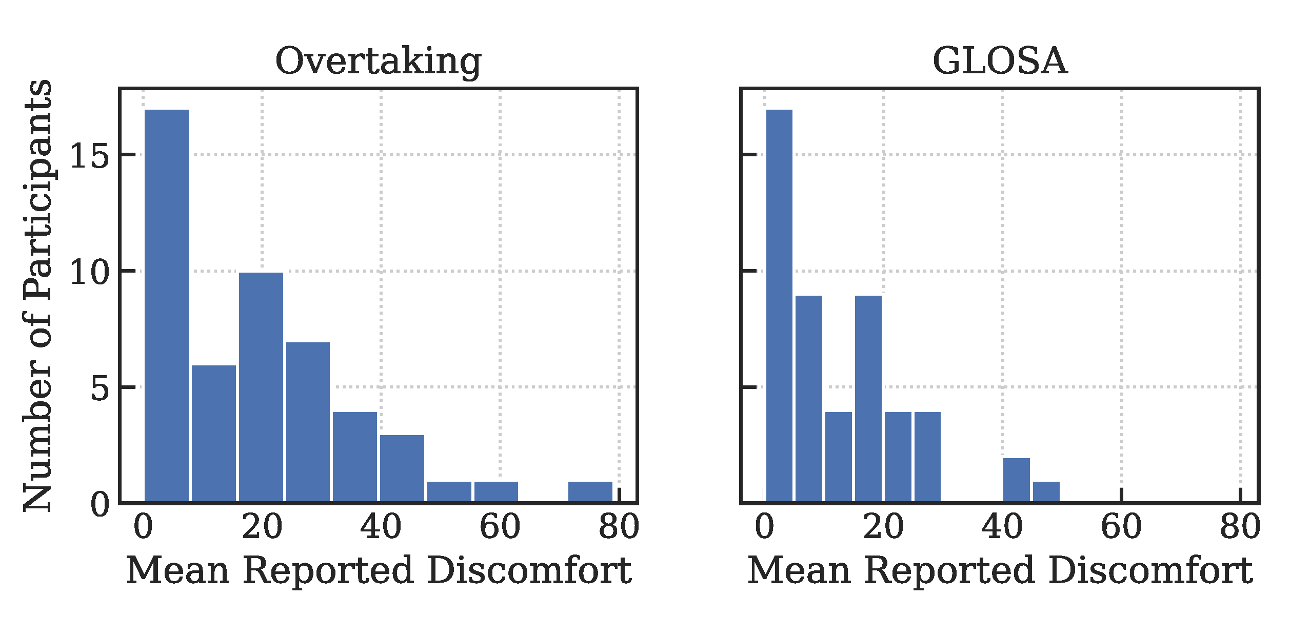
As exemplary driving scenarios with a high potential for passenger discomfort, modelling was focused on the overtaking scenarios (see Figure 3: around 0.8 and km 3.2) and the GLOSA scenarios (see Figure 3: around km 2.0 and km 2.5) (see Section 2.1 for scenario descriptions). Figure 4 provides an overview of the averaged discomfort values indicated during these scenarios per participant. In comparison, the bypassing scenarios were perceived as even more uncomfortable than the GLOSA scenarios.

3.2. User State Modelling Approaches

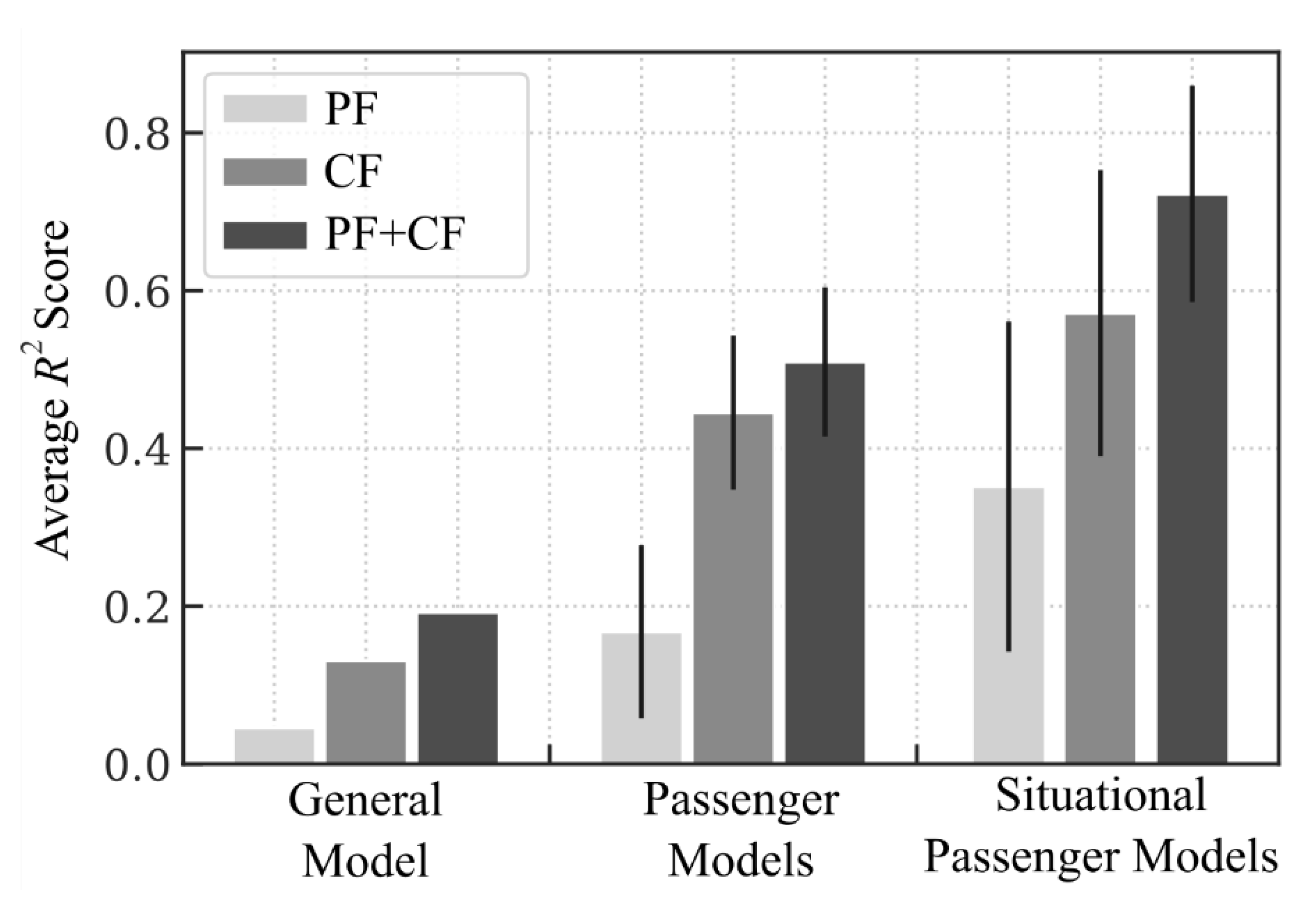
As shown in the previous section, the discomfort responses of the participants varied greatly across all scenarios. In this section, we investigate how different approaches for model training affect the overall performance of predicting passenger discomfort. Our three approaches are: (1) general model: training one model for the whole data set (all participants and all situations), (2) passenger models: training a separate model for each participant (one participant each, all situations) and (3) situational passenger models: training a separate model for each participant and each situation, which was carried out on the examples of the overtaking and GLOSA scenarios. To determine the importance of the passenger features and the accompanying sensory requirements, all of these approaches were done respectively using only PF, only CF and both feature sets. For modelling, we scaled the reported discomfort values from range (0, 100) to range (0, 1).

The resulting $R^2$ scores of the three approaches are displayed in Figure 5. The first approach, training one model for the whole data set (general model), yields the worst score. Even with PF and CF used, the score of the model is below 0.2. This shows that one model cannot accurately describe the relationships between features and discomfort of all participants.

Therefore, the second approach (passenger models) is more suitable for predicting passenger discomfort. Since one model is trained here for each participant (‘participant models’), each model can focus on the participants’ individual discomfort responses to the environment and more accurately describe the relationships between features and reported discomfort. Because multiple models are trained in this approach, Figure 5 now displays the average score all of these models, with the respective SD as error bar. As displayed, the performance of these models reaches 0.51 ± 0.09 in the best case (using PF and CF).

Our third approach uses additional knowledge that can originate from the AV, namely the current contextual situation, and uses it to create situation-specific passenger models as explained in Section 2.3. The idea is to create multiple simple models that only operate within a certain contextual scope. This approach increases performance because each model has to consider only contextualized feature–target-relationships. In Figure 5, the scores are displayed, averaged over both scopes and all participants. As shown, the performance increases to a score of up to 0.72 ± 0.14 using PF and CF. This absolute score cannot be compared directly to the scores of the other two approaches, because only a subset of data is modelled. However, the full data set would be predicted by using the model from approach 2, when no overtaking maneuver or GLOSA situation is given, and the situational passenger model approach, when these situations occur. This way, the overall score would lay between the two approaches, depending on how often these situations occur. Besides the performance increase, the situational passenger models can fit feature–target-relationships, which are specific for their respective scenario, without needing to adhere to all other scenarios. These specific relations can be used for explainability, which will be more precise than the more general models. Using the SHAP method, we will subsequently analyze the different relationships between discomfort and features calculated by the situational passenger models in comparison to the personal model approach, and will cover the topic of explainability.

As shown with the $R^2$ scores, models that work purely with CF do not perform well, since the discomfort values indicated by different participants vary greatly across contextually similar situations. Thus, the addition of passenger features and the approach of training one model per participant increases performance through the usage of participants’ individual feature responses instead of the average response over all participants.

Figure 6 illustrates these improvements for a section of the time series data of one overtaking scenario for three participants. From left to right, the examples show an increasingly larger difference between CF and CF + PF, i.e., on the left is only a very minor improvement noticeable, on the right a larger one. In all three cases, the CF model predicts the situations of discomfort with less precision than the model using CF + PF. It predicts discomfort with less temporal accuracy, i.e., the discomfort value is higher for times where no discomfort was reported and also does not predict the reported discomfort magnitude as precise as the CF + PF model.

3.3. Model Explanation

As mentioned, the situational passenger model approach leads to more specific modelling and thus to better explainability. We now use the SHAP method to analyze how the features influence the prediction and how this influence varies across the general model and the situational passenger model approach. For this purpose, we use the SHAP summary plot explained in Section 2. For the situational passenger model approach, we pooled together all SHAP values from all participants, since we have 50 models to be looked at. This can lead to non-linearly appearing relationships between features and model output, which are in fact just inter-participant differences of the models.

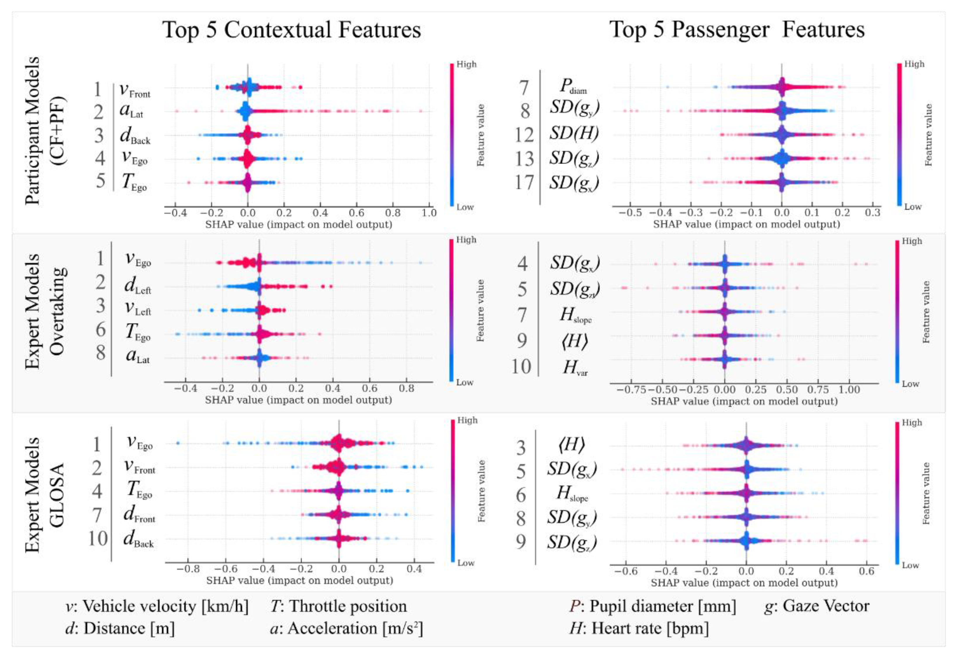
For this analysis, we use three different model types: the participant models (Figure 7, first row) and the situational passenger models for overtaking (Figure 7, second row) as well as GLOSA (Figure 7, third row). For each of these model types we show the SHAP summary plots with the top 5 contextual features (first column) and the top five passenger features (second column), according to the SHAP value rating. Next to the feature symbols are the ranking numbers for the according feature in the combined ranking, i.e., CF + PF. This ranking is the sum of the according absolute SHAP values for each feature.

It can be noted that most of the SHAP value distributions have very long tails and are not normal distributed. This results from the short moments of maneuvers in relation to the whole study duration where discomfort is reported and the SHAP values being most relevant in these situations. Thus, most data points over the duration of the ride have SHAP values close to zero and only a few have extreme values.

To demonstrate how the situational passenger model approach increases explainability and changes the feature–target relations in contrast to the participant models, we analyze the situational passenger model SHAP values and the participant models’ SHAP values of the contextual features. In Figure 7 top row, the SHAP values of the participant models are shown. The most important feature over all participants is the velocity of the vehicle in front of the ego vehicle $v_{Front}$, which increases the discomfort the higher the velocity gets, for most of the participants. The lateral acceleration $a_{Lat}$ is especially important when very high, as seen on the second rank with the very long tail towards the higher model output impacts. The following features are the distance to the vehicle behind the ego vehicle $d_{Back}$, the velocity of the ego vehicle $v_{Ego}$, and the throttle of the ego vehicle $T_{Ego}$. These variables, although important, do not share a common relationship across all participants; low values of one feature can impact the model output either positively or negatively. Overall, in these models which have to take into account data of the whole ride, very general features, for example speed, lateral acceleration, and distance, the front and back vehicles are most important.

To show how an expert model changes the feature importance and relationships to discomfort prediction, the situational passenger models for overtaking are displayed in the second row. Here, the most important feature is $v_{Ego}$, which is not only increased from rank 4 in comparison to the participant models, but now also with a very strong negative correlation to the model output. When overtaking, low speeds are associated with high discomfort. An interpretation of this will follow below. The next most important features are the distance $d_{Left}$ and velocity $v_{Left}$ to the opposing traffic vehicle on the left lane. This shows a strong relation to overtaking maneuvers, since the lane crossing into opposing traffic is a strong cause for discomfort. These two features do not occur within the top ranks of the participant models, showing that they are not important enough during the whole ride. This is understandable, since an overtaking maneuverer typically does not last long in comparison to the ride duration. The same principle applies to the situational passenger models for GLOSA scenarios. Here, $v_{Ego}$ is again the most important feature, but the direction of influence is switched with regards to the overtaking manoeuvre. Also, one can notice an increase in the importance of features related to the vehicle directly in front of the ego vehicle, thus now the velocity $v_{Front}$ and the distance $d_{Front}$ are on rank 2 and 4. The importance of the front vehicle is expected in GLOSA scenarios, since a sudden brake of this vehicle in response to a red light is a potential hazard. These two examples demonstrate that different maneuvers and scenarios cannot be captured by general, cross-situational models, and how expert models select more situation-specific features. Notice that these explanations occur without putting any more knowledge into the model, but only the correct contextual data split. Thus, this approach is scalable to large amounts of data and arbitrary more contexts.

The SHAP method also allows for interpreting the features in regard to the model impact direction, which proved to be a challenging task, but also gives lots of insights on how complex further interpretation of sensor data can be. For example, the feature $d_{Left}$ in the overtaking expert model has a positive relation to the model output: The larger the distance between ego vehicle and the left lane opposing vehicle, the more discomfort is predicted. This seems unintuitive at first, since one would expect close distances to induce higher discomfort. However, in the general, in a safely driven overtaking scenario, a passenger experiences the highest discomfort in the initial stages of the maneuver (when approaching the obstacle on the own lane), when the oncoming vehicle on the left lane typically is still far away. At this stage, discomfort is induced by the decreasing distance to the obstacle on the own lane and the passenger’s uncertainty about whether or not the automation will initiate the overtaking maneuver in time. In contrast, the distance to the oncoming traffic on the left lane is the smallest when the obstacle is already safely bypassed and discomfort is therefore removed, resulting in a statistical association between a small distance and low discomfort. Another exemplary feature in this model is $v_{Ego}$. According to the model, lower speed is associated with higher predicted discomfort. This seems unintuitive at first, but can again be explained by the discomfort reasons during the initial stages of this scenario. Thus, the vehicle is reducing speed slightly before initiating the overtaking process, when passenger discomfort is at its highest point. When the vehicle is at normal speeds again, the overtaking is already in process, and the passenger’s uncertainty regarding the obstacle is already dissolved. This is contrary to the GLOSA expert model, where high levels of $v_{Ego}$ cause high discomfort, which makes sense because the ego vehicle is moving towards a red light, thus it should slow down to reduce discomfort. These examples show how difficult an analysis of the impact direction of the features is. It does not only depend on the scenario and the human response to it, but also can be complicated by indirect relations between perceived discomfort and certain context features, which make the automatic modelling using the SHAP method even more useful.

The passenger features also contribute significantly to the model output, although generally not as much as the contextual features. In the participant models, the SHAP importance for PF is starting at rank 7 with the pupil diameter $P_{diam}$. Overall, in the PF data, we observe larger differences in contrast to the CF across the participants: Many PF have different directions of impact on the models. These differences coupled with the low amounts of data in the situational passenger models leads to poor quality SHAP results for situational passenger models for Overtaking and GLOSA. Therefore, we will concentrate on the participant approach for the PF analysis.

As mentioned, over the whole ride, the pupil diameter is the best passenger-related predictor for discomfort. Across all participants, the larger the diameter, the more discomfort was reported, which is consistent with previous statistical analyses of this relationship [3]. Additionally, the next best predictor is the standard deviation of the y component of the gaze vector SD($g_y$). For all participants, the lower this value, the more discomfort was reported. This suggests the fixation of the eye onto certain objects on the simulator screen. The next passenger feature is the standard deviation of the heart rate SD(H), although the high values of both suggest low and high discomfort, which suggests that the participants heart rate did not react in the same way to discomfort across all participants. A more detailed data analysis with more data should be conducted to analyze this relationship more thoroughly. Similarly, the SHAP values of all passenger features in the situational passenger models are very noisy and do not show a clear direction in their relation to discomfort. We believe that this is due to the fact that the PF are overall noisier than the CF and thus need more observations to be fitted correctly.

Overall, the eye-related PF over the whole ride shows a strong, directed relation to discomfort over all participants, which suggests that an eye tracking device should be applied to future studies and application context and combined with contextual feature loggers to enhance the prediction of discomfort.

4. Discussion

The results of our three model approaches show a major improvement from method one (training one model for all participants) to method two (training one model for each participant). This, in combination with the results from the SHAP method, suggests to use the second, passenger-based method in future applications. It allows to train models for every passenger of a vehicle and to create a learning model for each passenger that adapts to only that passenger, without being influenced by other humans. In combination with the used explanation method, this also gains passenger specific insights about possible driving features that are correlated with the measured uncertainty.

A more detailed explanation would be given by the third method, where models are trained not only per passenger, but also for a selected number of driving maneuvers. This however, was problematic in our work, because of the few data that remains after such specific data splits. Although the performance of the models increased, which is often the case when modelling less data, the SHAP method showed very poor results, which proves that the amount of data was too small and we thus could not focus on the results in this work. However, we still believe this method is promising and it should be investigated further on a bigger data set in future research. Collecting a data set that is magnitudes bigger than our training set is not unlikely in practice, since in privately owned cars a single person can easily accumulate hundreds of driving hours within a few months, and it should thus be possible to outperform our results in a long-term vehicle usage.

One challenge concerning the measuring of discomfort is the need of sensors that are often attached to the body of the passengers, hindering them in their mobility and comfort, and thus reducing the probability of a positive user experience. Therefore, the high predictor results of the pupil-related sensors are of special interest, since a camera based measurement approach could work without contact to the passengers and without hindering their mobility or the need to put something onto their body before driving, which results in a very practical application scenario.

For data analysis, the SHAP methods proved to be a very promising tool to analyze the correlations in the data models. However, even when using linear models, some of the discovered relations were hard to put into context, which showed how difficult further interpretation and modelling of the results might be. Seemingly easy to interpret features, for instance the distance to an approaching car, can completely change meaning to the passenger based on the driving context. Future research is needed in this field to create models that can fully model and help to understand these relations.

When a sufficient understanding of the feature relations is given, we believe that it is possible to infer driving style changes from these relations. Using our results from the SHAP method, each feature can be used individually to improve driving styles and reduce discomfort. For example, a high lateral acceleration $a_{Lat}$ in the passenger models is very often related with higher values of discomfort, as seen in Figure 7. Thus, it is easy to infer that $a_{Lat}$ should be reduced. One can also deduce out of the data how much $a_{Lat}$ has to be reduced for every participant by using the SHAP values. We expect the same to be possible for every feature and for every maneuver if the maneuver models are trained on enough data. Thus, an automatic and model based driving style adaption specific for every driver could be implemented in future autonomous vehicles using this method.

5. Conclusions

For this work, we conducted a driving simulator study to investigate human discomfort while driving autonomously through inner city scenarios. We demonstrated that participants’ discomfort experiences vary greatly across different scenarios, and that one general model cannot predict discomfort across all scenarios and participants. Thus, we used two different approaches: training one model for one passenger, and also training such passenger-specific models for single types of driving scenarios. We found that in comparison with a general model, both approaches increased prediction performance greatly. The latter approach creates multiple expert models which are used only in their respective scenario, thus even simple linear models are able to make precise predictions. We used the SHAP method to investigate which features of the environment affected discomfort the most and how the use of expert models specializes this influence. We found that the expert models can create better explanations for discomfort, since they only operate on a specific type of driving scenario. These scenario-specific explanations could be used by the vehicle to adapt the driving style or in-vehicle information presentation in that scenario accordingly to reduce passenger discomfort.

We also quantified to which degree the use of passenger state features improves the model performance of all of our approaches and, using the SHAP method, which of these features contribute most to the prediction of discomfort. Our analysis demonstrates that eye tracking data is most important for the models and thus a promising tool to effectively increase the discomfort prediction performance without obstructing the passenger.

In future research, our approaches may be applied to more diverse simulated scenarios or to real-world driving studies to enhance the generalizability and external validity of our results. A study with a real autonomous vehicle would be of special interest to confirm the possibility of the mixture of expert approach, since the vehicle’s sensory data could be evaluated for automatic scenario classification.

References

1. Drewitz, U.; Ihme, K.; Bahnmüller, C.; Fleischer, T.; La, H.; Pape, A.A.; Gräfing, D.; Niermann, D.; Trende, A. Towards user-focused vehicle automation: The architectural approach of the AutoAkzept project. In International Conference on Human-Computer Interaction; Springer: Cham, Switzerland, 2020; pp. 15–30. [Google Scholar]
2. Dettmann, A.; Hartwich, F.; Roßner, P.; Beggiato, M.; Felbel, K.; Krems, J.; Bullinger, A.C. Comfort or not? Automated driving style and user characteristics causing human discomfort in automated driving. Int. J. Hum. Comput. Interact. 2021, 37, 331–339. [Google Scholar] [CrossRef]
3. Beggiato, M.; Hartwich, F.; Krems, J. Using Smartbands, Pupillometry and Body Motion to Detect Discomfort in Automated Driving. Front. Hum. Neurosci. 2018, 12, 338. [Google Scholar] [CrossRef] [PubMed]
4. Radhakrishnan, V.; Merat, N.; Louw, T.; Lenné, M.; Romano, R.; Paschalidis, E.; Hajiseyedjavadi, F.; Wei, C.; Boer, E. Measuring Drivers’ Physiological Response to Different Vehicle Controllers in Highly Automated Driving (HAD): Opportunities for Establishing Real-Time Values of Driver Discomfort. Information 2020, 11, 390. [Google Scholar] [CrossRef]
5. Azevedo-Sa, H.; Jayaraman, S.K.; Esterwood, C.T.; Yang, X.J.; Robert, L.P.; Tilbury, D.M. Real-Time Estimation of Drivers’ Trust in Automated Driving Systems. Int. J. Soc. Robot. 2020, 1–17. [Google Scholar] [CrossRef]
6. Dommel, P.; Pichler, A.; Beggiato, M. Comparison of a Logistic and SVM Model to Detect Discomfort in Automated Driving. In International Conference on Intelligent Human Systems Integration; Springer: Cham, Switzerland, 2021; pp. 44–49. [Google Scholar]
7. Trende, A.; Hartwich, F.; Schmidt, C.; Fränzle, M. Improving the detection of user uncertainty in automated overtaking maneuvers by combining contextual, physiological and individualized user data. In International Conference on Human-Computer Interaction; Springer: Cham, Switzerland, 2020; pp. 390–397. [Google Scholar]
8. Hartwich, F.; Schmidt, C.; Gräfing, D.; Krems, J.F. In the passenger seat: Differences in the perception of human vs. automated vehicle control and resulting HMI demands of users. In HCI in Mobility, Transport, and Automotive Systems. Automated Driving and In-Vehicle Experience Design; Krömker, H., Ed.; Springer: Cham, Switzerland, 2020; pp. 31–45. [Google Scholar] [CrossRef]
9. Lundberg, S.; Lee, S.-L. A unified approach to interpreting model predictions. arXiv 2017, arXiv:1705.07874. [Google Scholar]
10. Hartwich, F.; Beggiato, M.; Krems, J.F. Driving comfort, enjoyment and acceptance of automated driving—Effects of drivers’ age and driving style familiarity. Ergonomics 2018, 61, 1017–1032. [Google Scholar] [CrossRef] [PubMed]
11. Beggiato, M. Changes in Motivational and Higher Level Cognitive Processes When Interacting with In-Vehicle Automation. Ph.D. Dissertation, University of Technology Chemnitz, Chemnitz, Germany, 2015. Available online: http://nbnresolving.de/urn:nbn:de:bsz:ch1-qucosa-167333 (accessed on 7 June 2021).
12. Borst, C.; Wieling, W.; Van Brederode, J.F.; Hond, A.; De Rijk, L.G.; Dunning, A.J. Mechanisms of initial heart rate response to postural change. Am. J. Physiol. Circ. Physiol. 1982, 243, H676–H681. [Google Scholar] [CrossRef] [PubMed]
13. Walocha, F.; Drewitz, U.; Ihme, K. Activity and Stress Estimation Based on OpenPose and Electrocardiogram for User-Focused Level-4-Vehicles. In review.
14. Malik, M.; Bigger, J.T.; Camm, A.J.; Kleiger, R.E.; Malliani, A.; Moss, A.J.; Schwartz, P.J. Heart rate variability: Standards of measurement, physiological interpretation, and clinical use. Eur. Heart J. 1996, 17, 354–381. [Google Scholar] [CrossRef] [Green Version]
15. Kret, M.E.; Sjak-Shie, E.E. Preprocessing pupil size data: Guidelines and code. Behav. Res. 2019, 51, 1336–1342. [Google Scholar] [CrossRef] [PubMed]
16. Montanari, F.; German, R.; Djanatliev, A. Pattern Recognition for Driving Scenario Detection in Real Driving Data. In Proceedings of the 2020 IEEE Intelligent Vehicles Symposium (IV), Las Vegas, NV, USA, 19 October–13 November 2020; pp. 590–597. [Google Scholar] [CrossRef]
17. Wang, W.; Ramesh, A.; Zhu, J.; Li, J.; Zhao, D. Clustering of Driving Encounter Scenarios Using Connected Vehicle Trajectories. IEEE Trans. Intell. Veh. 2020, 5, 485–496. [Google Scholar] [CrossRef] [Green Version]
18. Jacobs, R.A.; Jordan, M.I.; Nowlan, S.J.; Hinton, G.E. Adaptive Mixtures of Local Experts. Neural Comput. 1991, 3, 79–87. [Google Scholar] [CrossRef] [PubMed]
19. Beggiato, M.; Hartwich, F.; Roßner, P.; Dettmann, A.; Enhuber, S.; Pech, T.; Gesmann-Nuissl, D.; Mößner, K.; Bullinger, A.C.; Krems, J. KomfoPilot—Comfortable automated driving. In Smart Automotive Mobility; Springer: Cham, Switzerland, 2020; pp. 71–154. [Google Scholar]
20. Hartwich, F.; Hollander, C.; Johannmeyer, D.; Krems, J. Enhancing passenger experience and trust in automated vehicles through user-adaptive HMIs: “The more the better” does not apply to everyone. Front. Hum. Dyn. 2021. in press. Available online: https://www.frontiersin.org/articles/10.3389/fhumd.2021.669030/abstract (accessed on 7 July 2021).
Figure 1. Driving simulator (left) with participant and sensor set-up: MS Band 2 (left), SMI Eye Tracking Glasses 2 (left), and handset control [8] (left and right).
Vehicles 03 00045 g001
Figure 2. Example SHAP value representation for one prediction (top) and SHAP summary plot for multiple predictions (bottom) with features f 1 , …, f n . The summary plot only shows the top 4 features.
Vehicles 03 00045 g002
Figure 3. Development of handset control values of 50 participants over the course of the test track. Higher values correspond to higher perceived discomfort.
Vehicles 03 00045 g003
Figure 4. Histograms of the mean reported discomfort from all participants over the overtaking (left) and GLOSA (right) scenario.
Vehicles 03 00045 g004
Figure 5. Comparison of model approaches. Averaged R2 scores over model approach. For each model approach, three feature sets are evaluated (passenger features (PF), contextual features (CF), and PF + CF). Error bars show the SD of the average score over models. The general model has no error bars, because it is only one model for each feature set and thus does not require averaging.
Vehicles 03 00045 g005
Figure 6. Three examples of discomfort over time. Each plot displays 3 discomfort values for one participant and for the same overtaking scenario. The discomfort values are the self-reported discomfort (labelled as target), the situational passenger model’s predictions only using CF, and the situational passenger model’s prediction using CF + PF. The time is relative to the beginning of the overtaking maneuver.
Vehicles 03 00045 g006
Figure 7. Six SHAP summary plots, each containing all 50 participants. The three rows contain different model approaches. The data is split, where each column only shows SHAP values of CF and PF, respectively. Next to each feature is a number that shows the importance ranking in the combined (CF + PF) feature set.
Vehicles 03 00045 g007
Publisher’s Note: MDPI stays neutral with regard to jurisdictional claims in published maps and institutional affiliations.