Abstract
This article presents a novel methodology to predict the optimal adaptive cruise control set speed profile (ACCSSP) by optimizing the engine operating conditions (EOC) considering vehicle level vectors (VLV) (body parameter, environment, driver behaviour) as the affecting parameters. This paper investigates engine operating conditions (EOC) criteria to develop a predictive model of ACCSSP in real-time. We developed a deep learning (DL) model using the NARX method to predict engine operating point (EOP) mapping the VLV. We used real-world field data obtained from Cadillac test vehicles driven by activating the ACC feature for developing the DL model. We used a realistic set of assumptions to estimate the VLV for the future time steps for the range of allowable speed values and applied them at the input of the developed DL model to generate multiple sets of EOP’s. We imposed the defined EOC criteria on these EOPs, and the top three modes of speeds satisfying all the requirements are derived at each second. Thus, three eligible speed values are estimated for each second, and an additional criterion is defined to generate a unique ACCSSP for future time steps. A performance comparison between predicted and constant ACCSSP’s indicates that the predictive model outperforms constant ACCSSP.
1. Introduction
The introduction of automobiles into the world inculcated innovation in many aspects of engineering, including design and manufacturing (Townsend and Calantone, 2014) [1]. Engineers worldwide continuously strive to develop cutting-edge technologies to augment the riders’ comfort, traffic behaviour, enhance safety and fuel economy (Katzenbach, 2015) [2]. In the current scenario, advanced features which include forward collision, traction control, and lane change, augment the safety, whereas the fuel economy drive mode reduces the fuel consumption. Among the features integrated into the vehicle, the ACC system developed by Labuhn and Chundrlik, 1995 played a vital dual role, in affecting safety and EOC [3]. The intricate concept of the ACC system is to produce controlled acceleration without disengaging the cruise in the user-defined proximity and strictly follow the user command of set speed (Marsden et al., 2001) [4]. Additionally, we could conclude from the existing literature (Mahdinia et al., 2020) that the activation of ACC results in lower IFCR [5]. Therefore, activating the ACC feature for traversing long trips would augment EOC.
However, identifying the optimal ACCSSP by considering the dynamic state of the vehicle for a definite coordinate on the terrain is an unsolved, challenging task for engineers. Researchers have performed the parametric optimisation of ACC output in the existing literature by analysing the real-time data of behaviour, traffic congestion, terrain data, and environmental factors. Stanton et al., 2005, Hoedemaeker et al., 1998, Kesting et al., 2007, Rudin-Brown et al., 2004, Moon et al., 2008, and Rosenfeld et al., 2015 considered driver behaviour as the key input to develop the control algorithm using analytical techniques and to tune the outputs of the ACC system [6,7,8,9,10,11]. The enhancements of vehicle connectivity opened doors to obtain real-time traffic congestion information. Milanés et al., 2013:2014, Kesting et al., 2008:2007, and Ploeg et al., 2011, adopted the DL models to estimate the ACCSSP and desired acceleration based on the traffic congestion data retrieved in real-time [12,13,14,15]. Li et al., 2017, Lu et al., 2019, Vedam, 2015, Kolmanovsky and Filev, 2010, Gáspár and Németh, 2014:2011:2013, and Ma et al., 2019, adopted the terrain data to estimate the ACC control parameters to reduce IFCR using the known mathematical models [16,17,18,19,20,21,22,23].
Existing techniques rely on either one or two affecting factors as inputs to predict ACCSSP considered, but none of the researchers included all the factors in conjunction to the best of our knowledge. Recently, we developed a DL model mapping all the VLV and EOP (Kolachalama et al., 2021) [24]. This DL model produced the best results for the ACC activated test case and included all the factors mentioned above, excluding traffic congestion information. This paper applied predefined EOC criteria to the predicted EOP, and the optimal ACCSSP is estimated corresponding to augmented EOC. We validated the proposed model using the real-time test vehicle data-driven road segments that included arterial, state ways, and freeways. The below sections show the detailed procedure adopted.
2. Predictive Model for EOP
We adopted the commonly available DL methods, NARX and LSTM, to develop predictive models involving time-sensitive data (Diaconescu, 2008) [25]. Kolachalama et al., 2021, compared NARX and LSTM methods using the real-time test case (2019 Cadillac XT6) and proved that the NARX method outperforms the LSTM model [24]. Hence, in this research, a similar NARX DL model is used with default training options to predict EOP, as shown in Table 1.

Table 1.
Prediction of EOP—NARX DL model.
As mentioned in the previous section, Figure 1 depicts the DL model to predict the EOP mapping VLV. The outputs of the DL model consist of the elements IET, IES, and IFCR, and the VLV, which embed with driver behaviour, body module parameters, environmental factors, and terrain data. The DBV consists of three elements speeding (Speed, LOT), steering (YAR, LAT) and CAT (Kolachalama et al., 2021) [24,26]. The parameters odometer, tire pressure, curvature, and gradient affect the vehicle traction, whereas CAT and EAT influence thermal stress on the engine (Kolachalama et al., 2008) [27]. Additionally, there is no loss of generality in replacing the gradient with the vehicle posture’s Euler angles, which affect the traction under no-slip (Eathakota et al., 2010) [28,29].
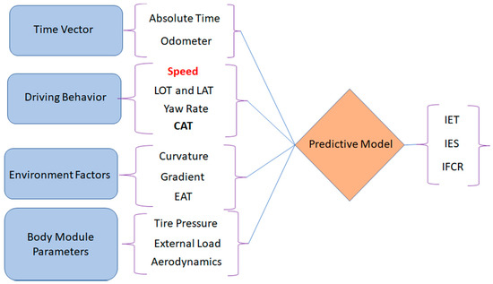
Figure 1.
Predictive model—inputs and outputs [5].
3. Metric for Optimal EOC
In this section, we defined the metrics for EOC criteria, which reflect optimal EOP.
3.1. Generic Criteria
The predicted EOP for the vehicles traversing the speeds ranging [25 45] MPH (arterial roads) have a closer proximity to the ideal EOP. In this scenario, the IET has a higher magnitude; on the contrary, for the speeds ranging [65 85], MPH (freeways) have higher IES recorded.
Additionally, the allowable speeds for the state ways range between [45 65] MPH are considered the green zone with maximum fuel economy (low IFCR). Hence, the generic criteria for augmented EOC would include higher IET, higher IES, and lower IFCR, along with the maximum distance traversed for the trip.
3.2. Euclidean Distance—Ideal EOP
An engine map calibrated at the manufacturing plant for every model by all automotive OEM’s represents the engine’s performance. In general, the ideal EOP for any vehicle represents the coordinate (centroid) on the map with the lowest IFCR. An example of the engine map for the vehicle 2014 Chevrolet 4.3L EcoTec3 LV3 Engine is shown in Figure 2A. The ideal EOP for this vehicle was estimated to be the coordinate [285 Nm, 2250 RPM, 225 g/kwh]. Similarly, the ideal EOPs for the three test vehicles are empirically estimated, as shown in section A: Table 2.
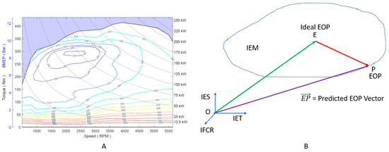
Figure 2.
(A) Engine map: 2014 Chevrolet 4.3L; (B) IEM—EOC vector. Environmental Protection Agency, National Vehicle and Fuel Emissions Laboratory, National Center for Advanced Technology, Ann Arbor, Michigan, USA. Version 2018-08.
Table 2.
EOC criteria—EOP.
Hence, we defined the line segment conjoining the predicted and ideal EOP as the EOC vector, represented by the IEM shown in Figure 2B. The magnitude of the EOC vector represents the shown in Equation (1). In the 2D plane, there is no loss of generality in ignoring the parameter IES, as it is proportional to the vehicle speed. Therefore, lower ED represents increased EOC.
3.3. Engine Caliber—Speed and Torque
The engine’s capability is measured by two standard parameters [ESC, ETC]. These parameters are the ratios that define the torque produced per unit of fuel consumption and the speed produced per unit of torque. Higher ETC and ESC are the desired criteria for every vehicle’s trip.
3.4. Smoothness Measure—EOC Parameters
The combustion of fuel in the engine produces torque with fluctuating magnitudes. However, all the elements of EOP should have smooth behaviour (Tanaka et al., 1987, Li et al., 2017) [30,31]. Hence, as an additional optimal EOC metric, we defined the smoothness measure for all the six parameters—IET, IES, IFCR, ED, ETC, ESC. We used the spline to fit the data points of EOC parameters by normalising the data. The optimal fit criteria were measured by traditional statistical techniques /Adjusted , RMSE, and SSE, using the built-in toolboxes of MATLAB as shown in section B: Table 2.
4. Prediction of ACCSSP
The prediction of ACCSSP was categorised into four steps, as described in the following sections.
4.1. Estimation of Future Input States—DL Model
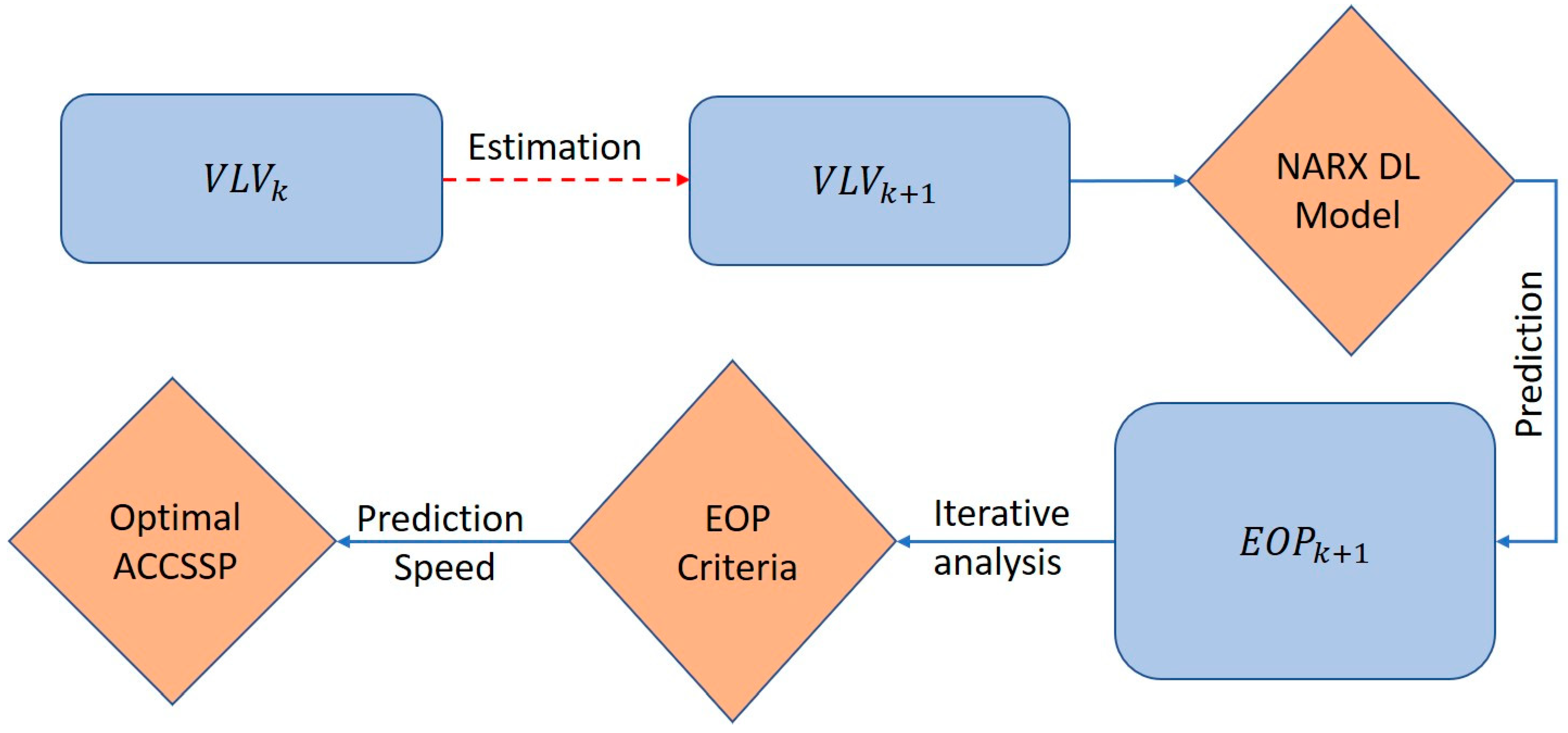
Step 1: Relative to the current state of the vehicle (), the future input values () of the DL model (Figure 3) are estimated using the relations shown in Table 3. The parameter odometer () was calculated using the speed () with the constant time step by basic linear interpolation. The LOT () is estimated based on the vehicle resistance shown in the equation set in Table 3, and the parameters YAR () and LAT () are calculated assuming ISB (Kolachalama et al., 2018) [25]. The environmental parameters , terrain data, [, ], are retrieved using the GPS location and the infotainment maps. The magnitudes of the tire pressure () and are assumed to be equal to the previous time step (Table 4).
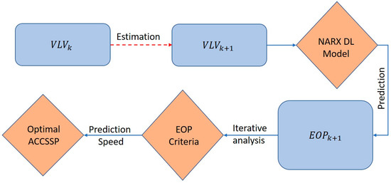
Figure 3.
Process—Prediction of optimal ACCSSP.
Table 3.
Equation set—prediction of future input states.
Table 4.
Predicted inputs—DL model, 2019 Cadillac XT6 (100 time steps = 1 s).
4.2. Prediction of Outputs—DL Model
Step 2: We estimated the input sets for future time steps (1 s—[ ]) for the AVS range (e.g., [SL-10, SL]). Thus, we generated eleven sets of inputs, and fed them into the DL model, and predicted a corresponding eleven sets of outputs (EOP’s) (Table 5).
Table 5.
EOC criteria—iteration of ACC Speeds (100 time steps).
4.3. Estimation of ACC Speed Values—EOC Criteria
Step 3: We applied the EOC criteria defined in section III for the eleven predicted EOP’s (Table 5). The top six performing speed values are selected for each EOC parameter, and hence, the top three modes of speeds (EVS) are calculated for each time step (Table 6). We incorporated a similar procedure for the next ten seconds, and the ACC Matrix (3X10) was developed (Table 7).
Table 6.
Eligible ACC speeds—EOC criteria (100 time steps = 1 s).
Table 7.
ACC speeds—10 s, SL = 75 MPH.
4.4. Algorithm to Predict ACCSSP
Step 4: Every second has three EVS, resulting in a maximum of possible ACCSSP’s for 10 s. The following conditions are defined to identify a unique ACCSSP inspired by the Dubin path traverse problem (La Valle, 2011) [32].
- Assuming the ACCSSP at is , if the EVS is either +1, , or −1, the highest magnitude among the three is selected as ;
- is chosen closer to (IAS). If this results in two values, then the higher value is considered as ;
- If the eligible speeds at are neither + 1, , nor − 1, then ;
- If for more than 10 s, = + 1 if + 1 SL or − 1 if = SL.
5. Experimental Results
A series of experiments are designed, analysed and evaluated on a real-time dataset to evaluate the performance of the proposed framework.
5.1. Dataset Retrieval
We conducted this research using three test vehicles, a 2019 Cadillac XT6, a 2020 Cadillac CT5, and a 2021 Cadillac CT4, obtained from GMC. A two-step procedure was employed to retrieve the data from the vehicle CAN bus (Li et al., 2008) [33]. We connected the hardware neoVI to the vehicle and retrieved the data retrieval using the software Vehicle Spy. This tool records data in real-time (Gallardo, 2018) and allows the user to selectively retrieve the signal data required for analysis [34]. We performed the real-time test procedure by activating the ACC feature, and time-step snippets of data were collected for each vehicle at a frequency of 10 Hz, i.e., 100 data points are recorded for 1s assuming a no-slip (Eathakota et al., 2008) [28,29].
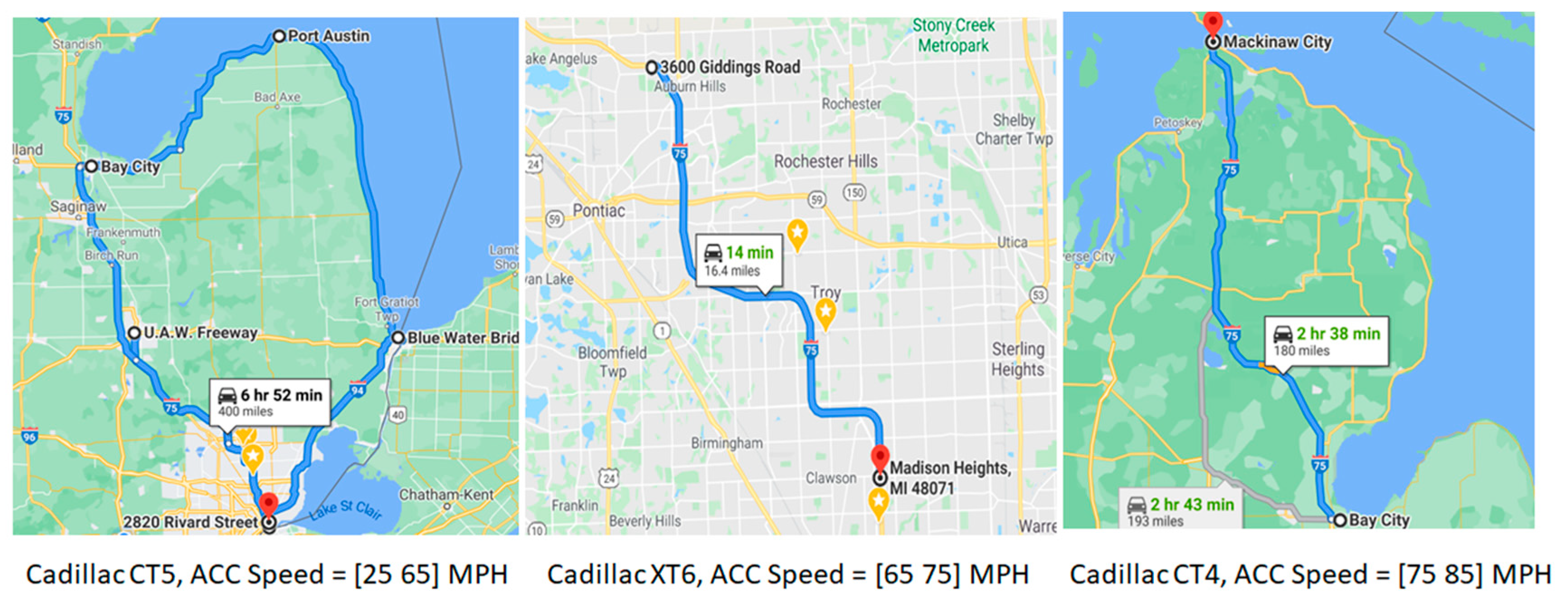
The test cases are developed by driving the vehicles on selected road segments covering all the arterial, state ways, and freeways scenarios. Shown in Figure 4 are the paths traversed by the Cadillac test vehicles. The properties of the six datasets used for this analysis, including the input and output parameters of the DL model, are shown in Table 8, Table 9 and Table 10. Please find the details of the predictive model in the following sections.
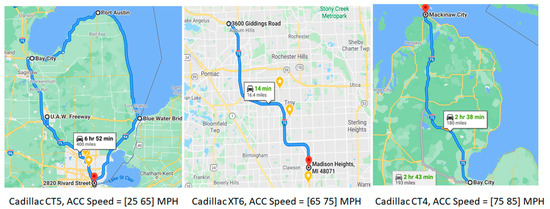
Figure 4.
Path traversed—GMC test vehicles (Google Maps).
Table 8.
Data Set 1: 2020 Cadillac CT5—arterial roads.
Table 9.
Data Set 2: 2020 Cadillac CT5—state ways roads.
Table 10.
Data Set 3: 2019 Cadillac XT6, 2021 Cadillac CT4—freeways roads.
5.2. Prediction of EOP
The properties of the NARX model and the test cases used for training are shown in Table 1. We developed individual training networks with default properties using the DL toolbox of MATLAB for the three vehicles’ test data and the predicted EOP’s, as shown in the Supplementary Materials, Figures S1–S6. Each figure consists of three parts: IET (left), IES (middle), and IFCR (right). Furthermore, each plot compares the measured data (blue) with the predicted values (orange). We validated the performance of the NARX DL model prediction using traditional statistical techniques (RMSE, FOD, SNR) to compare the actual and predicted values of EOP, as reported in Table 11. We conclude that IES follows a smooth curve, whereas IFCR and IET oscillate.
Table 11.
NARX DL model performance—ACCSSP [30 80] MPH.
5.3. Estimation of Optimal ACCSSP
The developed DL model and the steps defined in Section 4 are used to estimate the optimal ACCSSP for each test case. An example, for the test case of the vehicle 2019 Cadillac XT6, is selected with the AVS = [65 75] MPH, and the corresponding results are shown in Table 4, Table 5 and Table 6. The IAS () is varied in the range [65 75] MPH for the ACC Matrix (Table 7), and Step 4 is applied to the EVS, which results in eight ACCSSP’s shown in Figure 5. Thus for = 70 MPH, the predicted ACCSSP is the row vector ((71, 71, 71, 71, 72, 72, 73, 73, 74, 74) MPH) as shown in Figure S8. We adopted a similar procedure for multiple data sets and plotted the predicted ACCSSP’s are presented in the Supplementary Materials, Figures S7–S12. Please find the performance of EOC parameters for the predicted ACCSSP’s in Section B: Table 12.
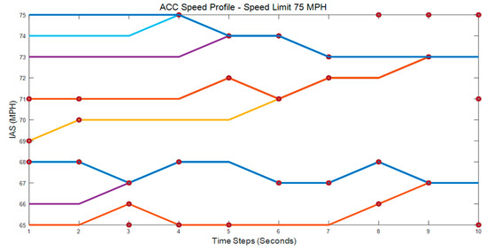
Figure 5.
Predicted ACCSSP, IAS = [65 75] MPH, SL = 75 MPH.
Table 12.
EOC criteria: engine parameters (predicted–constant) ACCSSP.
6. Discussion
The plots of predicted EOP’s for the three test vehicles Cadillac CT5, XT6, and CT4, are depicted in Figures S1–S6 The predictive model is validated by estimating the conformance between actual and predicted data’s RMSE, FOD, and SNR (Table 11). The IET RMSE values were <2.76, whereas IES FOD was <1.54 for all the datasets. We recorded the IFCR on a scale of 1 × 10⁻⁸ , and the IFCR SNR has an acceptable range of [24.41–30.36]. Additionally, we can visualise that the predicted curves have a smoother fit to the actual data, and thus efficacy of the DL model to predict EOP is validated.
In this work, we proposed the criteria for augmented EOC and an iterative methodology to predict ACCSSP’s, resulting in optimal EOP. Hence, for each future second, the AVS is varied in a definite range [65 75] MPH for the 2019 Cadillac XT6, and the corresponding inputs for the future states are fed into the DL model to generate multiple EOPs. We applied EOC criteria to the EOPs, and the top three EVS are estimated as [69,71,68] MPH.
We adopted a similar procedure for ten seconds and predicted ACCSSP for IAS = 70 MPH, SL = 75 MPH, with a minimum of 71 MPH and a maximum of 73 MPH (Figure S8). The predicted and constant ACCSSP profile (70 MPH) with corresponding inputs (Section 4.1) were fed into the DL model to obtain two different EOP’s vectors (Section 4.2) for future time steps (10 s). We applied the EOC criteria for the two EOPs whose values are in Section A: Table 12 and thus predicted ACCSSP resulted in 934.77 m of the additional distance traversed and a reduced ED of 373.968. Additionally, the constant ACCSSP = 70 MPH consumed 379.095 1 × 10⁻⁸ more fuel in 10 s compared with the predicted ACCSSP.
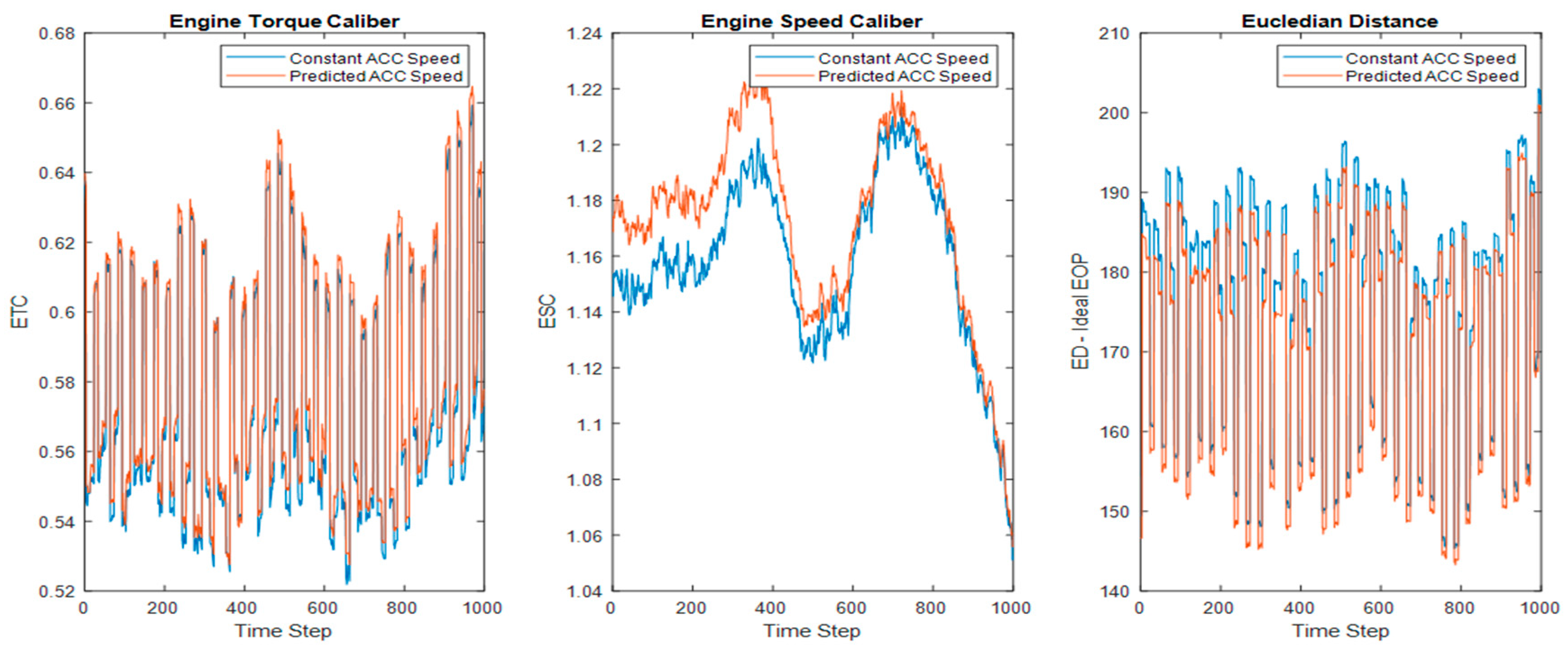
The plots of engine performance parameters are shown in Figure 6, and the area under the curve has higher magnitudes by 1.2 (ETC) and 10.2 (ESC) for the predicted ACCSSP. Please find the smoothness measure for the conformance of the two EOP’s in Table 13, and /Adjusted have similar values (conformance~ 0), whereas RMSE/SSE have lower values for predicted ACCSSP for most cases. Section B: Table 12 depicts the performance of EOC parameters for all the test cases, and it is easy to see that in most cases, the predicted ACCSSP has reduced ED and IFCR. Hence the proposed approach in this article is novel and better suits enhancing EOC and lowering the trip time.
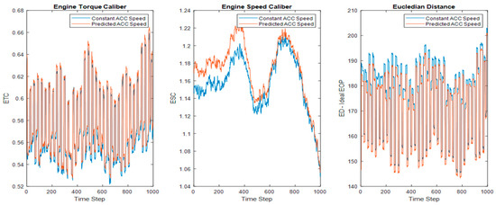
Figure 6.
EOC Parameters—(ETC, ESC, ED); IAS = 70 MPH, SL = 75 MPH, 2019 Cadillac XT6.
Table 13.
EOC criteria: smoothness performance—(predicted–constant) ACCSSP.
7. Conclusions and Future Work
In this manuscript, we developed a novel method to predict the ACCSSP, which optimises engine performance. We considered the vector EOP and used NARX DL modelling techniques to predict the EOP by mapping the VLV. We defined EOC criteria using the elements of EOP, which reflect enhanced engine operating conditions. In this methodology, a new approach of inputting the range of allowable ACC speeds is proposed and, therefore, a unique ACCSSP for the future time-steps was generated in the defined range by utilising iterative methods and satisfying the EOC criteria. The predicted and constant ACCSSP are fed into the DL model, and the engine performance parameters are estimated based on the predicted EOP. The results depict that for predicted ACCSSP, the parameters (ETC, ESC, IET, IES), and (IFCR, ED) have higher and lower values. Additionally, the predicted ACCSSP generated smoother profiles for the engine parameters when plotted in the time domain.
The researchers have not investigated the proposed technique of predicting ACCSSP, and this new approach could also trigger a new capability in ACC controllers to deviate from the user command of unique set speed and produce enhanced vehicle performance. The computational results obtained were satisfactory, and thus, we observed augmented EOC for the predicted ACCSSP.
We did not include many critical points, including traffic congestion, in the model. Future work would involve developing the model by including all the affecting parameters and performing extensive validation using multiple vehicle lines at various locations and periods. Additionally, this research could be extended to electric vehicles by defining new criteria of battery and motor operating conditions.
Supplementary Materials
The following are available online at https://www.mdpi.com/article/10.3390/vehicles3040044/s1, Figure S1: Prediction of EOP-ACCSSP = 30 MPH, 2020 Cadillac CT5; Figure S2: Prediction of EOP-ACCSSP = 40 MPH, 2020 Cadillac CT5; Figure S3: Prediction of EOP-ACCSSP = 50 MPH, 2020 Cadillac CT5; Figure S4: Prediction of EOP-ACCSSP = 60 MPH, 2020 Cadillac CT5; Figure S5: Prediction of EOP-ACCSSP = 70 MPH, 2019 Cadillac XT6; Figure S6: Prediction of EOP-ACCSSP = 80 MPH, 2021 Cadillac CT4; Figure S7: Prediction of ACCSSP-IAS = 80 MPH, SL = 85 MPH; Figure S8: Prediction of ACCSSP-IAS = 70 MPH, SL = 75 MPH; Figure S9: Prediction of ACCSSP-IAS = 60 MPH, SL = 65 MPH; Figure S10: Prediction of ACCSSP-IAS = 50 MPH, SL = 55 MPH; Figure S11: Prediction of ACCSSP-IAS = 40 MPH, SL = 45 MPH; Figure S12: Prediction of ACCSSP-IAS = 30 MPH, SL = 35 MPH.
Author Contributions
The first author (S.K.) came up with the idea, developed the concept, and performed the analysis. The second author (H.M.) is the principal investigator for this project. All authors have read and agreed to the published version of the manuscript.
Funding
The project “Predictive model of ACCSSP” was performed under the University of Michigan and GMC research collaboration, funded by William J. Clifford (Director) of the Systems Engineering department at GMC.
Institutional Review Board Statement
Not applicable.
Informed Consent Statement
Not applicable.
Data Availability Statement
The data used in this work are proprietary to GMC and cannot be made publicly available. However, the modelling algorithm is available on request.
Acknowledgments
The authors would like to thank Iqbal Surti, Systems Engineer at GMC, for his assistance in real-time testing. The technical analysis was performed using the tools provided by GMC (Vehicle Spy and neoVI) and the University of Michigan (MATLAB).
Conflicts of Interest
The authors of this manuscript declare that there is no conflict of interest regarding the publication of this article.
Abbreviations
| ACC | Adaptive cruise control | |
| ACCSSP | Adaptive cruise control set speed profile (MPH) | |
| Area | Area under the curve | |
| AVS | Allowable vehicle speeds | |
| CAN | Controller area network | |
| CAT | Cabin air temperature (°F) | |
| DL | Deep Learning | |
| DBV | Driver behaviour vector | |
| EAT | External air temperature (°F) | |
| ED | Euclidean distance—Ideal EOP and Predicted EOP | |
| EOC | Engine operating conditions | |
| EOP | Engine operating point | |
| ESC | Engine speed caliber | |
| EVS | Eligible vehicle speeds | |
| ETC | Engine torque caliber | |
| FOD | First order derivative | |
| IAS | Initial ACC speed (MPH) | |
| IEM | Instantaneous engine map | |
| IES | Instantaneous engine speed (rad/s) | |
| IET | Instantaneous engine torque (Nm) | |
| IFCR | Instantaneous fuel consumption rate (1 × 10⁻⁸ ) | |
| ISB | Ideal steering behaviour | |
| LAT | Lateral acceleration (m· ) | |
| LOT | Longitudinal acceleration (m·) | |
| LSTM | Long short-term memory | |
| GMC | General motors corporation | |
| MPH | Miles per hour | |
| MY | Model year | |
| NARX | Autoregressive network with exogenous inputs | |
| OEM | Original equipment manufacturer | |
| RMSE | Root mean square error | |
| RRC | Radius of road curvature (m) | |
| SL | Speed limit (MPH) | |
| SNR | Signal to noise ratio | |
| SSEStdDev | Sum of squared errorsStandard deviation | |
| TP | Tire pressure (kPa) | |
| TPFL | Tire pressure front left (kPa) | |
| TPFR | Tire pressure front right (kPa) | |
| TPRL | Tire pressure rear left (kPa) | |
| TPRR | Tire pressure rear right (kPa) | |
| VLV | Vehicle level vectors | |
| YAR | Yaw rate (rad/s) | |
Nomenclature
| Area of vehicle cross-section () | |
| Aerodynamic drag coefficient | |
| °F | Fahrenheit |
| g | Gravity |
| Hz | Hertz |
| kPa | Kilopascals |
| Kg | Kilogram |
| Km | Kilometres |
| kWh | Kilowatt-hour |
| Lateral acceleration at time step k (m·) | |
| Longitudinal acceleration at time step k (m·) | |
| Mass of the vehicle. (Kg) | |
| Mass of the additional load (Kg) | |
| MPH | Miles per hour |
| m | Meters |
| Meter square (measure of area) | |
| Meter cube per second (volume rate flow) | |
| m. | Meters per second square |
| ms | Milli seconds |
| Nm | Newton meter |
| Rolling coefficient | |
| rad | Radians |
| rad/s | Radians per second |
| Radius of road curvature at time step k (m) | |
| RPM | Rotations per minute |
| Density of air (kg.) | |
| s | Seconds |
| Timestep | |
| Incremental time step (~10 ms) | |
| Gradient of the terrain at time step k (rad) | |
| Yaw rate at time step k (rad/s) | |
| Meter cube per second (Volume rate flow) |
References
- Townsend, J.D.; Calantone, R.J. Evolution and Transformation of Innovation in the Global Automotive Industry. J. Prod. Innov. Manag. 2014, 31, 4–7. [Google Scholar] [CrossRef]
- Katzenbach, A. Automotive. In Concurrent Engineering in the 21st Century; Springer: Cham, Switzerland, 2015; pp. 607–638. [Google Scholar]
- Labuhn, P.I.; Chundrlik, W.J., Jr. Adaptive Cruise Control. U.S. Patent 5,454,442, 3 October 1995. [Google Scholar]
- Marsden, G.; McDonald, M.; Brackstone, M. Towards an understanding of adaptive cruise control. Transp. Res. Part C Emerg. Technol. 2001, 9, 33–51. [Google Scholar] [CrossRef]
- Mahdinia, I.; Arvin, R.; Khattak, A.J.; Ghiasi, A. Safety, Energy, and Emissions Impacts of Adaptive Cruise Control and Cooperative Adaptive Cruise Control. Transp. Res. Rec. J. Transp. Res. Board 2020, 2674, 253–267. [Google Scholar] [CrossRef]
- Stanton, N.A.; Young, M.S. Driver behaviour with adaptive cruise control. Ergonomics 2005, 48, 1294–1313. [Google Scholar] [CrossRef] [Green Version]
- Hoedemaeker, M.; Brookhuis, K. Behavioural adaptation to driving with an adaptive cruise control (ACC). Transp. Res. Part F Traffic Psychol. Behav. 1998, 1, 95–106. [Google Scholar] [CrossRef]
- Kesting, A.; Treiber, M.; Schönhof, M.; Kranke, F.; Helbing, D. Jam-avoiding adaptive cruise control (ACC) and its impact on traffic dynamics. In Traffic and Granular Flow’05; Springer: Berlin, Heidelberg, 2007; pp. 633–643. [Google Scholar]
- Rudin-Brown, C.M.; Parker, H.A. Behavioural adaptation to adaptive cruise control (ACC): Implications for preventive strategies. Transp. Res. Part F Traffic Psychol. Behav. 2004, 7, 59–76. [Google Scholar] [CrossRef]
- Moon, S.; Yi, K. Human driving data-based design of a vehicle adaptive cruise control algorithm. Veh. Syst. Dyn. 2008, 46, 661–690. [Google Scholar] [CrossRef]
- Rosenfeld, A.; Bareket, Z.; Goldman, C.V.; Leblanc, D.J.; Tsimhoni, O. Learning Drivers’ Behavior to Improve Adaptive Cruise Control. J. Intell. Transp. Syst. 2015, 19, 18–31. [Google Scholar] [CrossRef]
- Milanes, V.; Shladover, S.E.; Spring, J.; Nowakowski, C.; Kawazoe, H.; Nakamura, M. Cooperative Adaptive Cruise Control in Real Traffic Situations. IEEE Trans. Intell. Transp. Syst. 2013, 15, 296–305. [Google Scholar] [CrossRef] [Green Version]
- Milanés, V.; Shladover, S.E. Modeling cooperative and autonomous adaptive cruise control dynamic responses using experimental data. Transp. Res. Part C Emerg. Technol. 2014, 48, 285–300. [Google Scholar] [CrossRef] [Green Version]
- Kesting, A.; Treiber, M.; Schönhof, M.; Helbing, D. Adaptive cruise control design for active congestion avoidance. Transp. Res. Part C Emerg. Technol. 2008, 16, 668–683. [Google Scholar] [CrossRef]
- Ploeg, J.; Serrarens, A.F.A.; Heijenk, G.J. Connect & Drive: Design and evaluation of cooperative adaptive cruise control for congestion reduction. J. Mod. Transp. 2011, 19, 207–213. [Google Scholar] [CrossRef] [Green Version]
- Lin, D.-Y.; Hou, B.-J.; Lan, C.-C. A balancing cam mechanism for minimizing the torque fluctuation of engine camshafts. Mech. Mach. Theory 2017, 108, 160–175. [Google Scholar] [CrossRef]
- Lu, C.; Dong, J.; Hu, L. Energy-Efficient Adaptive Cruise Control for Electric Connected and Autonomous Vehicles. IEEE Intell. Transp. Syst. Mag. 2019, 11, 42–55. [Google Scholar] [CrossRef]
- Vedam, N. Terrain-Adaptive Cruise Control: A Human-Like Approach. Ph.D. Thesis, Texan A&M University, Collage Station, TX, USA, 2015. [Google Scholar]
- Kolmanovsky, I.V.; Filev, D.P. Terrain and Traffic Optimized Vehicle Speed Control. IFAC Proc. Vol. 2010, 43, 378–383. [Google Scholar] [CrossRef]
- Gaspar, P.; Németh, B. Design of adaptive cruise control for road vehicles using topographic and traffic information. IFAC Proc. Vol. 2014, 47, 4184–4189. [Google Scholar] [CrossRef] [Green Version]
- Németh, B.; Gáspár, P. Road inclinations in the design of LPV-based adaptive cruise control. IFAC Proc. Vol. 2011, 44, 2202–2207. [Google Scholar] [CrossRef] [Green Version]
- Németh, B.; Gaspar, P. Design of vehicle cruise control using road inclinations. Int. J. Veh. Auton. Syst. 2013, 11, 313. [Google Scholar] [CrossRef] [Green Version]
- Ma, J.; Hu, J.; Leslie, E.; Zhou, F.; Huang, P.; Bared, J. An eco-drive experiment on rolling terrains for fuel consumption optimization with connected automated vehicles. Transp. Res. Part C Emerg. Technol. 2019, 100, 125–141. [Google Scholar] [CrossRef]
- Kolachalama, S.; Lakshmanan, S. Using Deep Learning to Predict the Engine Operating Point in Real-Time; SAE Technical Paper; General Motors LLC: Detroit, MI, USA, 2021. [Google Scholar]
- Diaconescu, E. The use of NARX neural networks to predict chaotic time series. Wseas Trans. Comput. Res. 2008, 3, 182–191. [Google Scholar]
- Kolachalama, S.; Hay, C.L.; Mushtarin, T.; Todd, N.; Heitman, J.; Hermiz, S. An Algorithm to Estimate Steering Behavior Using Vehicle Radius of Curvature; Research Disclosure, Questel Ireland Ltd.: Paris, France, 2018; p. 647068. [Google Scholar]
- Kolachalama, S.; Kuppa, K.; Mattam, D.; Shukla, M. Thermal Analysis of Radiator Core in Heavy Duty Automobile. In Proceedings of the Heat Transfer Summer Conference, Jacksonville, FL, USA, 10–14 August 2008; Volume 48487, pp. 123–127. [Google Scholar]
- Eathakota, V.P.; Kolachalama, S.; Krishna, K.M.; Sanan, S. Optimal posture control for force actuator based articulated suspension vehicle for rough terrain mobility. In Advances in Mobile Robotics; World Scientific: Coimbra, Portugal, 2008; pp. 760–767. [Google Scholar]
- Eathakota, V.; Singh, A.K.; Kolachalama, S.; Madhava Krishna, K. Determination of Optimally Stable Posture for Force Actuator Based Articulated Suspension for Rough Terrain Mobility. In Trends in Intelligent Robotics. FIRA 2010; Communications in Computer and Information Science; Springer: Berlin/Heidelberg, Germany, 2010; Volume 103. [Google Scholar]
- Tanaka, H.; Tokushima, T.; Higashi, H.; Hamada, S. Means for Suppressing Engine Output Torque Fluctuations. U.S. Patent 4,699,097, 13 October 1987. [Google Scholar]
- Li, S.E.; Guo, Q.; Xu, S.; Duan, J.; Li, S.; Li, C.; Su, K. Performance Enhanced Predictive Control for Adaptive Cruise Control System Considering Road Elevation Information. IEEE Trans. Intell. Veh. 2017, 2, 150–160. [Google Scholar] [CrossRef]
- La Valle, S.M. Motion planning. IEEE Robot. Autom. Mag. 2011, 18, 108–118. [Google Scholar] [CrossRef]
- Li, R.; Liu, C.; Luo, F. A design for automotive CAN bus monitoring system. In Proceedings of the 2008 IEEE Vehicle Power and Propulsion Conference, Harbin, China, 3–5 September 2008; pp. 1–5. [Google Scholar]
- Gallardo, F.B. Extraction and Analysis of Car Driving Data via Obd-II. Ph.D. Thesis, Universidad Miguel Hernández de Elche, Alicante, Spain, 2018. [Google Scholar]


Publisher’s Note: MDPI stays neutral with regard to jurisdictional claims in published maps and institutional affiliations. |
© 2021 by the authors. Licensee MDPI, Basel, Switzerland. This article is an open access article distributed under the terms and conditions of the Creative Commons Attribution (CC BY) license (https://creativecommons.org/licenses/by/4.0/).