Mean Extinction Times in Multi-Metastable Systems: A Discrete Coarse-Grained Approach

Abstract

The paper develops a coarse-grained framework for computing mean extinction times in multi-metastable systems modeled as one-step continuous-time Markov chains with an absorbing state. At the microscopic level, backward equations on finite corridors are solved to obtain closed-form series for committors, mean first-passage times, and intrawell (basin) waiting times. A renewal–reward construction then yields effective interwell transition rates written as a success probability divided by a mean cycle duration, providing an interpretable effective rate constant. These rates define a reduced Markov chain on the wells together with extinction; mean extinction times follow from a linear system, and the associated fundamental matrix quantifies pre-extinction residence times in each coarse state. This framework makes explicit how multiple escape pathways and intrawell dwell times contribute to extinction statistics in finite systems. The method is illustrated on a double-well landscape with an extinction state, using a reversible potential-to-rates mapping for the numerical example. Comparisons of alternative intrawell models and validation against exact one-step computations demonstrate accuracy at finite system sizes, including regimes where diffusion approximations are unreliable. The resulting formulas require only local rate data, remain numerically stable under strong bias, and extend directly to multiple wells and flexible boundary conditions.

1. Introduction

Escape and extinction are central to nonequilibrium physics, chemical kinetics, and quantitative biology [1,2,3]. A nanoscale magnet flips its orientation; a molecule crosses an energy barrier to react; an ion channel toggles between open and closed; a population or gene-expression state collapses to zero—each is a rare event that occurs after long residence in a “well”, followed by a quite quick transition across a barrier [3,4,5,6,7,8,9]. The characteristic observable for such problems is a mean time to extinction (MTE) or mean switching time from some long-lived state to an absorbing set (for example, zero population) [2]. Classic continuum theories (Kramers’ law and its descendants [1,5,6,10,11]) quantify these times for overdamped diffusions in smooth potentials, and have guided physics for decades; however, many modern systems are intrinsically discrete—such as molecule counts, binding sites, spin flips, ion-channel subunits—and the “natural” model class is a one-step (birth–death) continuous-time Markov chain (CTMC) on a finite or semi-infinite lattice [11,12,13,14]. In such chains, extinction is not a boundary layer of a PDE; it is exactly the absorbing state, and the rates between wells can be computed exactly using the algebra of one-dimensional Markov chains [2,13,14].

The advantages of using a discrete Markov chain are as follows. (i) Physical fidelity: in many domains (stochastic gene expression, ion-channel gating, receptor binding, spin flips), the state is a count or a small integer. Extinction is not infinitesimal “density near zero”; it is exactly the absorbing state 0 [4,7,8,9]. (ii) Analytical tractability: in one dimension, birth–death chains admit exact committors and mean first-passage times (MFPTs) in terms of scale/speed, with no small-noise or asymptotics required [2,13,14]. (iii) Numerical robustness: the series require only sums and products of rates; they remain stable even in strongly biased corridors, where PDE discretizations can be stiff [11,12]. (iv) Composability: when well-to-well rates are known, assembling the coarse-grained CTMC provides MTEs for any initial well with a single linear solution, which naturally extends to multiple wells and branching pathways [15,16].

The study uses a microscopic birth–death layer (one-step CTMC) in which it deals directly with the backward master equation on a finite corridor between two indices $L<R$, deriving closed-form series for (i) the splitting probability (committor denoted by q) to hit R before L, (ii) the mean first-passage time (MFPT denoted by T) to either boundary from any interior site, which is also the attempt duration, and (iii) one-sided intrawell exit times ($\Theta$) that capture the “waiting” inside a metastable basin before a corridor attempt begins [2,13,14]. These formulas are expressed through the classical scale and speed arrays for birth–death chains, which make the recurrences telescopic. The combination of committor, MFPT, and intrawell waiting gives an effective transition rate $k=q/(\Theta +T)$ from one well to the next via a renewal–reward argument [17,18]. Here, each renewal cycle consists of an intrawell waiting period followed by a corridor attempt; under the standard assumption that cycles are independent and identically distributed, k has the interpretation of an effective rate constant (successful transitions per unit time). Using effective transition rates as edges, a coarse-grained CTMC is assembled on the set of wells plus an absorbing extinction node. The MTE from any well is then the solution of the linear system $(-Q_T){\mathbb{T}}^e=\mathbf{1}$, where $Q_T$ is the generator restricted to the well states and ${\mathbb{T}}^e$ is the MTE. This follows the standard transient CTMC identity that the fundamental matrix ${(-Q_T)}^{-1}$ gives mean sojourn times in each state prior to absorption [15,16], yielding not only MTEs but also state-resolved residence times before extinction.

In contrast to discrete Markov chains, there are approximation techniques that are practical for solving the chain in the large system limit. Kramers–Eyring theory and matched asymptotics for overdamped diffusions provide expressions for barrier-crossing rates with exponential accuracy and prefactors that depend on curvatures at wells and saddles [1,10,11]. Another method is large-deviation/WKB (Wentzel–Kramers–Brillouin) methods for master equations (system-size expansions, WKB ansätze, optimal-path Hamiltonians) which deliver asymptotic estimates of extinction probabilities and times in many-body or multi-type processes [19,20]. These are practical and helpful when state spaces are high-dimensional and exact enumeration is not possible, and reveal optimal fluctuation paths to extinction. In transition path theory (TPT) and Markov state models (MSMs), the committor is central in TPT; on discrete spaces, it solves a linear system for Markov jump processes, and MSMs estimate coarse-grained rates from simulation and use TPT objects (fluxes, reactive densities) to analyze rare events [21,22,23,24].

The approach taken in this paper is complementary: first, one-step chains are used and the exact committor/MFPT and intrawell times are computed, giving non-asymptotic well-to-well rates; then, a relatively small coarse-grained CTMC delivers MTEs from any well, including full extinction.

The uniqueness of the approach used is to provide a unified exact workflow for discrete one-step systems that includes intrawell waiting (often omitted) and an absorbing extinction state; (a) a bridge that connects microscopic backward equations (scale/speed series) to a coarse-grained well graph with a backwards equation yielding MTEs and residence times; (b) a detailed worked example (double-well landscape) that shows how intrawell modeling (single-site vs. basin) shifts rates and how the coarse-grained solver aggregates them into extinction times; and (c) explicit formulas suitable for validation by simulation and for embedding in larger multiscale models.

The rest of this paper is organized as follows. The model is presented in Section 2 by introducing the one-step CTMC framework, including rate parameterizations, boundary conditions, and the identification of metastable wells through basins and corridors. Section 3 develops the microscopic corridor solution, providing exact derivations of committors and MFTPs to either boundary using scale and speed measures. In Section 4, the intrawell series and renewal logic for inter-well rates are derived. Section 5 focuses on extinction, presenting an exact series on a bounded interval and characterizing the extinction rate from the leftmost well in connection with quasi-stationarity. In Section 6, the analysis moves to a coarse-grained well graph where the generator is constructed with extinction states, solved via the fundamental matrix, and interpreted in terms of expected times. Section 7 illustrates the framework with a double well with an absorbing state example, offering end-to-end computations of rates and mean times to extinction (MTEs) along with model comparison with exact solutions. Finally, Section 8 discusses the physical mechanisms controlling MTEs, including the balance between success probabilities and intrawell waiting times, and places the results in the context of Kramers theory, WKB approximations, and transition path theory while also outlining other applications.

2. Model and Assumptions

The microscopic dynamics is modeled as a one-step (birth–death) CTMC on a finite lattice

$$\mathcal{S}=\{0,1,\dots ,n\},$$

with 0 reserved as a strictly absorbing extinction state. From any interior state $i\in \{1,\dots ,n-1\}$, the chain jumps to $i+1$ (a birth) at rate ${\lambda }_i\ge 0$ and to $i-1$ (a death) at rate ${\mu }_i\ge 0$. The generator of the process acts on bounded functions $f:\mathcal{S}\to \mathbb{R}$ as

$$\left(\mathcal{L}f\right)\left(i\right)={\lambda }_i\left(f(i+1)-f\left(i\right)\right)+{\mu }_i\left(f(i-1)-f\left(i\right)\right),i=0,1,\dots ,n,$$

(1)

with the conventions ${\lambda }_n=0$ under a reflecting right boundary (no jumps to $n+1$) and ${\lambda }_0={\mu }_0=0$ to enforce extinction at $i=0$; see [13,14] for background on birth–death chains.

2.1. Metastable Wells, Basins, and Corridors

It is assumed that the chain exhibits two or more long-lived (metastable) states (“wells”) $W_1<W_2<\cdots <W_m$ on $\{1,\dots ,n\}$. Operationally, a well W can be identified near a zero of the mean drift

$$b_i={\lambda }_i-{\mu }_i,$$

with $b_i$ changing sign so that the local drift points inward toward W (a discrete analogue of a stable fixed point). Around each well $W_k$ a basin $[a_k,W_k]$ is introduced to its left and $[W_k,c_k]$ to its right, used to quantify intrawell waiting (Section 4). For any pair of neighboring wells $L=W_k$ and $R=W_{k+1}$, the corridor

$$[L,R]=\{L,L+1,\dots ,R\},$$

is defined which is treated with absorbing endpoints at L and R when solving splitting/first-passage problems between the wells. In the special case of extinction from the leftmost well $W_1$, the relevant corridor is $[0,W_1]$ with absorbing endpoints at 0 and $W_1$.

2.2. Parameterizing the Rates: Custom Arrays vs. Reversible Mapping

The methodology used supports two complementary rate parameterizations:

(i)

Custom rate arrays

One may specify the non-negative arrays ${\left\{{\lambda }_i\right\}}_{i=0}^n$ and ${\left\{{\mu }_i\right\}}_{i=0}^n$ directly, subject to boundary conventions (for example, ${\lambda }_n=0$, ${\lambda }_0={\mu }_0=0$). This is appropriate when rates are measured or derived from a mechanistic micro-model [13,25].

(ii)

Reversible (local-symmetric) mapping from a discrete potential

Alternatively, given a discrete potential $U:\{0,\dots ,n\}\to \mathbb{R}$, an attempt frequency $\nu >0$, and an inverse temperature $\beta >0$, the local-symmetric assignment is adopted:

$${\lambda }_i=\nu exp\left[-\frac{\beta }{2}\left(U(i+1)-U\left(i\right)\right)\right],{\mu }_i=\nu exp\left[-\frac{\beta }{2}\left(U(i-1)-U\left(i\right)\right)\right]$$

(2)

for i in their ranges (with ${\lambda }_n=0$), which enforces detailed balance with respect to

$$\pi \left(i\right)\propto exp[-\beta U(i\left)\right],i=0,\dots ,n$$

so that $\pi \left(i\right){\lambda }_i=\pi (i+1){\mu }_{i+1}$ for all interior i [11,12]. Equation (2) is the discrete analogue of overdamped Langevin dynamics in U, and is used in the worked example considered. Other kinetic rules (Arrhenius one-sided, Metropolis) are possible but change stationary weights (and hence the exact series); comparisons must use identical mappings.

2.3. Boundary Policies and Extinction

The following boundary conventions are considered.

• Extinction at 0. ${\lambda }_0={\mu }_0=0$ is always imposed, making 0 absorbing.
• Right boundary at i = n. Reflecting (${\lambda }_n=0$, ${\mu }_n\ge 0$) is the default here; an absorbing right boundary (${\lambda }_n=0$, ${\mu }_n=0$) is also allowed and can model finite boxes; finally, “as-given” leaves $({\lambda }_n,{\mu }_n)$ unchanged if a different closure is physically motivated.

These choices affect corridors that reach n, but do not alter the left-extinction corridor $[0,W_1]$.

2.4. Scale and Speed Arrays on a Corridor

Fix $L<R$ and consider the corridor $[L,R]$ with L and R absorbing. Let

$${\tau }_L=inf\{t\ge 0:X_t=L\},{\tau }_R=inf\{t\ge 0:X_t=R\}$$

denote the first hitting times of the endpoints. The following variables are defined: the bias ratios $r_i$,

$$r_i={\displaystyle \frac{{\mu }_i}{{\lambda }_i}},L+1\le i\le R-1,$$

the scale weights $w_i$,

$$w_{L+1}=1,w_{i+1}=w_i{r}_i(L+1\le i\le R-1),$$

(3)

the cumulative scale $s_i$,

$$s_L=0,s_i=\sum _{k=L+1}^i{w}_k,L+1\le i\le R,$$

(4)

and the speed factors $e_i$,

$$e_i={\displaystyle \frac{1}{{\lambda }_i{w}_{i+1}}}(L+1\le i\le R-1).$$

(5)

The bias ratios $r_i={\mu }_i/{\lambda }_i$ measure the local tendency of the chain at site i to step left rather than right, i.e., the balance of backward to forward transition rates. From these ratios one builds the scale weights $w_i$, which recursively accumulate the product of biases along the chain and encode how the bias compounds across successive sites. Summing the weights gives the cumulative scale $s_i$, which provides a natural “coordinate” on the corridor that straightens out the bias; in particular, hitting probabilities (committors) reduce to simple linear functions of this scale variable. The speed factors $e_i=1/\left({\lambda }_i{w}_{i+1}\right)$ adjust for the absolute magnitude of the transition rates, correcting the scale information with the actual time scale of jumps; they are the ingredients that enter the explicit MFPT formulas. Together, scale ($r,w,s$) captures the geometry of biased motion, while speed (e) captures how fast the process moves; it can be shown that committors and mean times can be written exactly as series in these quantities.

A key identity is ${\lambda }_i{w}_{i+1}={\mu }_i{w}_i$, which follows directly from Equation (3). The classical theory shows that the committor and MFPT on $[L,R]$ can be written as explicit series in $w,s,e$ (no approximation) [2,13,14,26]. This identity follows from the scale-weight recursion and does not assume detailed balance of the CTMC. In what follows, these series are used to compute corridor success probabilities, attempt durations, and when combined with one-sided intrawell times, the effective well-to-well transition rates.

2.5. Intrawell Waiting Models

Rare transitions such as extinction occur as attempt cycles, i.e., an intrawell wait within the basin of a well to reach the corridor interface, followed by a single corridor attempt that either succeeds or fails. The followng two intrawell models are considered.

• Single-site intrawell. The basin of L is collapsed to the site L; the mean time to initiate a rightward attempt equals the mean waiting time for the specific right jump,

  $${\Theta }_L^{\left(\mathrm{ss}\right)}={\displaystyle \frac{1}{{\lambda }_L}}.$$

  (6)
  Symmetrically, ${\Theta }_R^{\left(\mathrm{ss}\right)}=1/{\mu }_R$.
• One-sided (basin) series. For a left basin $[a,L]$, ${\Theta }_L$ is the mean time to reach $L+1$ from L while confined to $[a,L+1]$ (absorbing at $L+1$), and admits a closed series in $w,s,e$. A symmetric construction yields ${\Theta }_R$ on a right basin $[R,c]$. These are exact one-sided MFPTs on half-corridors, and reduce to the single-site limits when $a=L$ or $c=R$.

Combining the corridor committor q and attempt duration (MFPT) T with intrawell times via renewal theory yields the macroscopic well-to-well rates derived in Section 4 [2,14].

2.6. Dimensions, Normalization, and Notational Summary

Rates ${\lambda }_i,{\mu }_i$ have units of inverse time. The arrays w and s are dimensionless (ratios of rates), while $e_i=1/\left({\lambda }_i{w}_{i+1}\right)$ has units of time. Let us list the principal notation used throughout:

${\lambda }_i,{\mu }_i$—birth/death rates at state i, either custom or from Equation (2);

$b_i={\lambda }_i-{\mu }_i$—mean drift used to locate wells;

$w_i$—scale weights on a corridor, via Equation (3);

$s_i$—cumulative scale, via Equation (4);

$e_i$—speed factors, via Equation (5);

$[L,R]$—corridor between two neighboring wells (absorbing endpoints);

$[a,L]$, $[R,c]$—left/right basins used for intrawell times;

${\tau }_L,{\tau }_R$—first hitting times of corridor endpoints L and R;

$q_i$—committor: ${\mathbb{P}}_i({\tau }_R<{\tau }_L)$ on $[L,R]$;

$T_i$—MFPT: ${\mathbb{E}}_i[min({\tau }_L,{\tau }_R\left)\right]$ on $[L,R]$;

${\Theta }_L,{\Theta }_R$—one-sided intrawell MFPTs to reach corridor interfaces;

$k_{L\to R}$—macroscopic transition rate between wells (renewal rate);

$k_{L^{-}\to 0}$—extinction rate from the leftmost well on $[0,L^{-}]$.

3. Corridor Committor and MFPT via Scale/Speed

The committor (also called the splitting probability) is a fundamental object in Markov chain theory and stochastic processes. Starting from i, it is the probability of the process reaching the right boundary R before the left boundary L. For a state i inside the corridor $[L,R]$, it is defined as

$$q_i={\mathbb{P}}_i({\tau }_R<{\tau }_L),$$

(7)

where ${\tau }_{L\left(R\right)}=inf\{t>0:S\left(t\right)=L\left(R\right)\}$ is the hitting time for the left (right) boundary and $S\left(t\right)$ denotes the state. It encodes the directional bias of the dynamics; $q_i\approx 1$ signifies that the chain is more likely to escape through the right, while $q_i\ll 1$ signifies escape through the left is much more probable. The committor is nonzero for $L<i<R$ with boundary values $q_L=0$ and $q_R=1$.

To obtain the governing relation for $q_i$, the backward equation is applied using first-step analysis. At state i, the chain waits an exponential time of mean $1/({\lambda }_i+{\mu }_i)$ before jumping either to $i+1$ with probability ${\lambda }_i/({\lambda }_i+{\mu }_i)$ or to $i-1$ with probability ${\mu }_i/({\lambda }_i+{\mu }_i)$. Conditioning on this first jump yields

$$q_i={\displaystyle \frac{{\lambda }_i}{{\lambda }_i+{\mu }_i}}{q}_{i+1}+{\displaystyle \frac{{\mu }_i}{{\lambda }_i+{\mu }_i}}{q}_{i-1}.$$

(8)

Multiplying through by $({\lambda }_i+{\mu }_i)$ gives the linear recurrence [11]

$${\lambda }_i(q_{i+1}-q_i)+{\mu }_i(q_{i-1}-q_i)=0.$$

(9)

To solve the recurrence [11], define the increments ${\Delta }_i=q_i-q_{i-1}$. Subtracting the equation at $i-1$ from the equation at i (equivalently rewriting Equation (9) in terms of increments) gives

$${\lambda }_i{\Delta }_{i+1}={\mu }_i{\Delta }_i,$$

and hence ${\Delta }_{i+1}=r_i{\Delta }_i$. This shows that the increments grow or shrink according to the local bias ratio. Iterating, one gets ${\Delta }_k={\Delta }_{L+1}{w}_k$, where $w_k={\prod }_{j=L+1}^{k-1}{r}_j$. Summing increments telescopically from $L+1$ to i and enforcing the boundary condition $q_L=0$ gives

$$q_i=\sum _{k=L+1}^i{\Delta }_k={\Delta }_{L+1}{s}_i,$$

(10)

where $s_i={\sum }_{k=L+1}^i{w}_k$ is the cumulative scale. The constant ${\Delta }_{L+1}$ is fixed by requiring $q_R=1$, which leads to the closed-form solution of the splitting probability

$$q_i={\displaystyle \frac{s_i}{s_R}},L<i<R.$$

(11)

Let us now consider the mean first-passage time to either boundary, which is also the attempt duration in a corridor $[L,R]$ with absorbing endpoints at L and R. It is defined as

$$T_i={\mathbb{E}}_i[\tau =min({\tau }_L,{\tau }_R\left)\right],\mathrm{with}{T}_L=T_R=0,$$

(12)

where ${\mathbb{E}}_i$ denotes expectation given $S\left(0\right)=i$. One can also define $\tau$ as

$$\tau =inf\{t>0:S\left(t\right)\in \{L,R\}\}\mathrm{with}{T}_i={\mathbb{E}}_i\left[\tau \right].$$

Starting from an interior state i, let $\sigma$ be the time for the first jump out of i and let $S\left(\sigma \right)\in \{i-1,i+1\}$ be the post-jump state. By the strong Markov property,

$$T_i={\mathbb{E}}_i\left[\tau \right]={\mathbb{E}}_i\left[\sigma \right]+{\mathbb{E}}_i\left[T_{S\left(\sigma \right)}\right].$$

(13)

A detailed derivation (increment transformation and telescoping) is provided in Appendix A; here, the following final closed-form expression is stated:

$$T_i={\displaystyle \frac{1}{s_R}}\sum _{k=L+1}^{R-1}{e}_k{s}_{min(i,k)}\left(s_R-s_{max(i,k)}\right),L<i<R,$$

(14)

where $min(i,k)$ ($max(i,k)$) denotes the smaller (larger) of the two indices, so that $s_{min(i,k)}=s_i$ and $s_{max(i,k)}=s_k$ when $i\le k$, and $s_{min(i,k)}=s_k$, $s_{max(i,k)}=s_i$ when $k<i$. Here, $s_{min(i,k)}$ captures how much “scale mass” lies to the left of the earlier of i and k. The factor $s_R-s_{max(i,k)}$ captures the remaining “scale mass” to the right of the latter of i and k. The speed $e_k=1/\left({\lambda }_k{w}_{k+1}\right)$ converts these geometric weights into physical time [27].

4. Intrawell Times and Renewal Rate

In many physical systems (magnetic grains, protein conformations, ion channels), most time is spent rattling inside a basin before a barrier-crossing attempt. Omitting intrawell waiting (reporting only the corridor attempt rate) can overestimate rates by an order-one factor when wells are broad. To make the model more realistic, intrawell waiting times are incorporated in the model under use. A rare $L\to R$ transition unfolds as attempt cycles consisting of (i) an intrawell wait to reach the corridor interface ($L\to L+1$), followed by (ii) one corridor attempt on $[L,R]$ that either succeeds (hit R) or fails (return to L). The right-to-left direction is symmetric with roles $L⟷R$ and interface $R-1$.

As mentioned in Section 2, there are two intrawell models under consideration in this study: (a) single-site and (b) one-sided basin (series). The intrawell means are computed by the same scale/speed machinery used in the calculation of MFPTs, but on half-corridors with one absorbing endpoint at the interface.

Let us first consider the left intrawell mean ${\Theta }_L$ (to initiate $L⟶R$). begin by choosing a left basin edge $a\le L$, for example by choosing the midpoint of the previous well, or $a=L$ for single-site. The chain is confined to $[a,L+1]$ with an absorbing boundary at $L+1$. This leads to the backward equation

$${\lambda }_i({\Theta }_{i+1}-{\Theta }_i)+{\mu }_i({\Theta }_{i-1}-{\Theta }_i)=-1,$$

(15)

with absorbing boundary condition ${\Theta }_{L+1}=0$. Solving exactly as in the MFPT case, one gets

$${\Theta }_L={\displaystyle \frac{w_{L+1}}{s_{L+1}-s_a}}\sum _{n=a+1}^L{\displaystyle \frac{s_n-s_a}{{\lambda }_n{w}_{n+1}}},$$

(16)

where $w_{a+1}=1$.

For the right intrawell mean ${\Theta }_R$ (to initiate $R⟶L$), a similar procedure is used here; a right basin cap $c\ge R$ is used and the chain to $[R-1,c]$ is confined with absorbing boundary at $R-1$. Using the same methodology as above, one gets

$${\Theta }_R={\displaystyle \frac{w_R}{s_c-s_{R-1}}}\sum _{n=R}^{c-1}{\displaystyle \frac{s_c-s_n}{{\lambda }_n{w}_{n+1}}}.$$

(17)

If the basin is collapsed to the well site L, the mean time to initiate a rightward attempt equals the mean waiting time for the specific right jump: ${\Theta }_L^{\left(\mathrm{ss}\right)}=1/{\lambda }_L$, or symmetrically, ${\Theta }_R^{\left(\mathrm{ss}\right)}=1/{\mu }_R$. Setting $a=L$ (or $c=R$) in Equation (16) (or Equation (17)) recovers the single-site limits.

4.1. Corridor Attempt Statistics

Consider the corridor $[L,R]$ with absorbing endpoints. An attempt is the excursion that starts at the moment the system enters the corridor at $i=L+1$ and ends when it hits either L (failure) or R (success). Its duration is

$$T_{L+1}={\mathbb{E}}_{L+1}\left[min({\tau }_R,{\tau }_L)\right],$$

(18)

which is the MFPT to either boundary. Between failed attempts, the chain waits inside the left well before returning to $L+1$ to try again. This is provided by the mean intrawell refresh time ${\Theta }_L$, which is the average time from a return to the left boundary L until the next entrance into the corridor at $L+1$. Thus, a full attempt cycle (fail → refresh → reenter → try again) has mean length

$${\mathbb{T}}_L={\Theta }_L+T_{L+1}.$$

(19)

Starting at $L+1$, the probability of exiting via R before L is the committor (splitting probability) provided by

$$q_{L+1}={\mathbb{P}}_{L+1}({\tau }_R<{\tau }_L)={\displaystyle \frac{s_{L+1}}{s_R}}={\displaystyle \frac{1}{s_R}},$$

(20)

where $s_{L+1}=w_{L+1}=1$. Each attempt can be treated as a Bernoulli trial with success probability $q_{L+1}$.

4.2. Renewal Rate

Define renewal times at the end of each attempt cycle (immediately after a failure returns to L and completes the intrawell refresh, or immediately upon success). Let $X_1,X_2,\dots$ be i.i.d. cycle lengths with expectation $\mathbb{E}\left(X_1\right)={\mathbb{T}}_L$. Let $Y_1,Y_2,\dots$ be the indicators that the corresponding attempt succeeds, with $\mathbb{E}\left(Y_1\right)=p=q_{L+1}$. Then, the number of successes by time t is given by

$$M\left(t\right)=\sum _{n=1}^{N\left(t\right)}{Y}_n,N\left(t\right)=max\{n:X_1+\cdots +X_n\le t\}.$$

(21)

By the elementary renewal–reward theorem under the standard assumption that cycles are independent and identically distributed [17,18],

$$\underset{t\to \infty }{lim}{\displaystyle \frac{M\left(t\right)}{t}}={\displaystyle \frac{\mathbb{E}\left[Y_1\right]}{\mathbb{E}\left[X_1\right]}}={\displaystyle \frac{q_{L+1}}{{\Theta }_L+T_{L+1}}}.$$

(22)

This long-time success throughput is the coarse-grained transition rate out of the left well, and has the interpretation of an effective rate constant

$$k_{L\to R}={\displaystyle \frac{q_{L+1}}{{\Theta }_L+T_{L+1}}}.$$

(23)

Symmetrically, starting attempts from the right entrance $R-1$ gives the success-to-left probability $1-q_{R-1}$ and cycle length ${\mathbb{T}}_R={\Theta }_R+T_{R-1}$; hence,

$$k_{R\to L}={\displaystyle \frac{1-q_{R-1}}{{\Theta }_R+T_{R-1}}}.$$

(24)

The corridor-only transition rates are obtained by substituting ${\Theta }_L={\Theta }_R=0$.

For later reference, the boundary-start MFPTs in the corridor are obtained from Equation (14). In particular,

$$\begin{array}{cc}\hfill T_{L+1}& ={\displaystyle \frac{1}{s_R}}\sum _{n=L+1}^{R-1}{e}_n(s_R-s_n),\hfill \end{array}$$

(25)

$$\begin{array}{cc}\hfill \hspace{1em}\hspace{1em}\hspace{1em}\hspace{1em}\hspace{1em}\hspace{1em} T_{R-1}& ={\displaystyle \frac{s_R-s_{R-1}}{s_R}}\sum _{n=L+1}^{R-1}{e}_n{s}_n={\displaystyle \frac{w_R}{s_R}}\sum _{n=L+1}^{R-1}{e}_n{s}_n.\hfill \end{array}$$

(26)

5. Extinction from the First Well ($W_1\to 0$)

Let us now consider extinction from the leftmost metastable well $L^{-}=W_1$. Let state 0 be absorbing. On the corridor $[0,L^{-}]$, the scale–speed arrays $w,s,e$ is built with base $w_1=1$ (so that $s_i={\sum }_{k=1}^i{w}_k$). A leftward extinction attempt is an excursion that starts upon entering the corridor at $i=L^{-}-1$ and ends when it hits either 0 (success) or returns to $L^{-}$ (failure).

The success probability for a leftward attempt starting at $L^{-}-1$ is

$$p_{\mathrm{succ}}={\mathbb{P}}_{L^{-}-1}({\tau }_0<{\tau }_{L^{-}})={\displaystyle \frac{s_{L^{-}}-s_{L^{-}-1}}{s_{L^{-}}}}={\displaystyle \frac{w_{L^{-}}}{s_{L^{-}}}}.$$

(27)

The mean duration of a leftward attempt is obtained using the same scale–speed machinery as in Appendix A. It is provided by

$$T_{L^{-}-1}^{[0,L^{-}]}={\displaystyle \frac{w_{L^{-}}}{s_{L^{-}}}}\sum _{n=1}^{L^{-}-1}{\displaystyle \frac{s_n}{{\lambda }_n{w}_{n+1}}}.$$

(28)

Let ${\Theta }_L^{-}$ be the mean time to initiate a leftward attempt (to hit $L^{-}-1$ starting from $L^{-}$), obtained as in Equation (17) with $R\mapsto L^{-}$ and the right basin cap chosen to the right of $L^{-}$. In the single-site model, ${\Theta }_L^{-}=1/{\mu }_{L^{-}}$.

Using the renewal logic of Section 4, the extinction rate is then

$$k_{L^{-}\to 0}={\displaystyle \frac{p_{\mathrm{succ}}}{{\Theta }_L^{-}+T_{L^{-}-1}^{[0,L^{-}]}}}={\left[\sum _{n=1}^{L^{-}-1}{\displaystyle \frac{s_n}{{\lambda }_n{w}_{n+1}}}+{\displaystyle \frac{s_{L^{-}}}{w_{L^{-}}}}{\Theta }_L^{-}\right]}^{-1}.$$

(29)

It has to be noted that this rate depends on the type of basin $[W_1,c^{-}]$.

6. Coarse-Grained Well Markov Chain

The coarse-grained well graph reduces the full microscopic birth–death chain to a much smaller CTMC defined only on the metastable wells together with an absorbing extinction state. Each metastable well $W_i$ is treated as a single coarse state, while extinction is modeled as the absorbing state 0. Transitions between wells are encoded by effective rates obtained from the microscopic corridor analysis in Section 3, Section 4 and Section 5, and extinction is included as an absorbing transition from the leftmost well. This coarse-grained CTMC captures the long-time dynamics of the original system while remaining analytically tractable.

The coarse-grained graph has the following state space and edges.

• Transient states. The transient states correspond to the metastable wells

  $$W=\{W_1<W_2<\cdots <W_m\},$$

  where each $W_i$ represents the basin of attraction of the ith metastable well.
• Absorbing state. Extinction is represented by the absorbing state 0.
• Edges and rates. The coarse-grained chain has two types of transitions.
  • Between neighboring wells. Effective transition rates are inherited from the microscopic corridor solutions

    $$k_{i,i+1}=k_{W_i\to W_{i+1}},k_{i+1,i}=k_{W_{i+1}\to W_i},1\le i\le m-1.$$
  • To extinction. The leftmost well $W_1$ transitions to extinction at a rate

    $$k_{1,0}=k_{L^{-}\to 0}=k_{W_1\to 0}$$

    computed from the microscopic corridor $[0,L^{-}=W_1]$.

Indexing wells by $i=1,\dots ,m$, the generator of the coarse-grained CTMC can be written in block form [16,28] as

$$Q=\left[\begin{array}{cc}{Q}_T& K_e\\ 0& 0\end{array}\right],$$

(30)

where $Q_T$ is the $m\times m$ subgenerator on the transient wells and $K_e$ is the $m\times 1$ column of extinction rates. The transient subgenerator $Q_T$ is tridiagonal, since transitions occur only between neighboring wells.

• For the leftmost well $i=1$:

  $$Q_T[1,2]=k_{1,2},Q_T[1,1]=-\left(k_{1,2}+k_{1,0}\right).$$
• For an interior well $1<i<m$:

  $$Q_T[i,i-1]=k_{i,i-1},Q_T[i,i+1]=k_{i,i+1},Q_T[i,i]=-\left(k_{i,i-1}+k_{i,i+1}\right).$$
• For the rightmost well $i=m$:

  $$Q_T[m,m-1]=k_{m,m-1},Q_T[m,m]=-k_{m,m-1}.$$

Thus, $Q_T$ has the structure of a one-dimensional chain with absorbing extinction through $W_1$ [15].

The MTE starting from well $W_i$ is obtained by solving the standard transient-CTMC linear system [16,28]

$$(-Q_T){\mathbb{T}}^e=\mathbf{1},$$

(31)

where ${\mathbb{T}}^e={(T_1^e,\dots ,T_m^e)}^{\top }$ is the vector of mean extinction times starting from each well state and $\mathbf{1}$ is a vector of ones. The unique solution is

$${\mathbb{T}}^e=N\mathbf{1},N={(-Q_T)}^{-1},$$

where N is the fundamental matrix. This is the standard mean sojourn time identity; $N_{ij}$ is the expected time spent in well $W_j$ before extinction when starting from well $W_i$ [15]. In particular:

• $T_i^e={\sum }_{j=1}^m{N}_{ij}$ is the mean time to extinction from $W_i$
• $N_{ij}$ is the expected occupation (residence) time in $W_j$ starting from $W_i$.

To illustrate the coarse-grained construction, explicit MTE formulas are worked out for $m=2$ and $m=3$ wells. These small cases are analytically tractable and serve as consistency checks.

6.1. MTE for Two Wells ($m=2$)

Let $k_{12}$, $k_{21}$, $k_{1,0}$ denote the effective rates

$$W_1\to W_2\mathrm{at}\mathrm{rate}{k}_{1,2},W_2\to W_1\mathrm{at}\mathrm{rate}{k}_{2,1},W_1\to 0\mathrm{at}\mathrm{rate}{k}_{1,0}.$$

The transient generator is

$$Q_T=\left(\begin{array}{cc}-(k_{1,2}+k_{1,0})& k_{1,2}\\ k_{2,1}& -k_{2,1}\end{array}\right),(-Q_T)=\left(\begin{array}{cc}{k}_{1,2}+k_{1,0}& -k_{1,2}\\ -k_{2,1}& k_{2,1}\end{array}\right).$$

(32)

The MTE vector ${\mathbb{T}}^e={(T_{W_1}^e,T_{W_2}^e)}^{\top }$ satisfies Equation (31). Solving gives

$$T_{W_1}^e={\displaystyle \frac{k_{1,2}+k_{2,1}}{k_{1,0}{k}_{2,1}}}={\displaystyle \frac{1}{k_{1,0}}}+{\displaystyle \frac{k_{1,2}}{k_{1,0}{k}_{2,1}}},T_{W_2}^e={\displaystyle \frac{k_{1,0}+k_{1,2}+k_{2,1}}{k_{1,0}{k}_{2,1}}}.$$

(33)

Some properties for the two wells are as follows.

• If $k_{1,2}\to 0$ (no hops to the right), then

  $$T_{W_1}^e\to {\displaystyle \frac{1}{k_{1,0}}},T_{W_2}^e\to {\displaystyle \frac{k_{1,0}+k_{2,1}}{k_{1,0}{k}_{2,1}}}={\displaystyle \frac{1}{k_{2,1}}}+{\displaystyle \frac{1}{k_{1,0}}}.$$
• If $k_{10}\to \infty$ (instant extinction once in $W_1$), then

  $$T_{W_1}^e\to 0,T_{W_2}^e\to {\displaystyle \frac{1}{k_{2,1}}}.$$

6.2. MTE for Three Wells ($m=3$)

Now, let $k_{1,2},k_{2,1},k_{2,3},k_{3,2},k_{1,0}>0$. The transient generator is

$$Q_T=\left(\begin{array}{ccc}-(k_{1,2}+k_{1,0})& k_{1,2}& 0\\ k_{2,1}& -(k_{2,1}+k_{2,3})& k_{2,3}\\ 0& k_{3,2}& -k_{3,2}\end{array}\right).$$

(34)

Again, Equation (31) holds with ${\mathbb{T}}^e={(T_{W_1}^e,T_{W_2}^e,T_{W_3}^e)}^{\top }$. Solving gives

$$\begin{array}{cc}\hfill T_{W_1}^e& ={\displaystyle \frac{k_{1,2}{k}_{2,3}+k_{1,2}{k}_{3,2}+k_{2,1}{k}_{3,2}}{k_{1,0}{k}_{2,1}{k}_{3,2}}},\hfill \\ \hfill T_{W_2}^e& ={\displaystyle \frac{k_{1,0}{k}_{2,3}+k_{1,0}{k}_{3,2}+k_{1,2}{k}_{2,3}+k_{1,2}{k}_{3,2}+k_{2,1}{k}_{3,2}}{k_{10}{k}_{2,1}{k}_{3,2}}},\hfill \\ \hfill T_{W_3}^e& ={\displaystyle \frac{k_{3,2}(k_{1,0}+k_{1,2})+(k_{1,0}+k_{1,2})(k_{2,1}+k_{2,3})-k_{1,2}{k}_{2,1}+k_{2,1}{k}_{3,2}}{k_{1,0}{k}_{2,1}{k}_{3,2}}}.\hfill \end{array}$$

(35)

Some limiting cases are as follows.

• If $k_{2,3}\to 0$ (well 3 decouples), the formulas reduce to the two-well system with wells $W_1,W_2$.
• If $k_{3,2}\to \infty$ (fast return from $W_3$), the additional time spent in $W_3$ vanishes and the system reduces effectively to two wells.

These explicit computations for $m=2$ and $m=3$ confirm the general structure: mean extinction times are rational functions of the effective coarse-grained rates, and the limiting behaviors match the expected physical intuition. In this way, the coarse-grained CTMC provides extinction times and occupation measures using only the effective transition rates computed in earlier sections.

7. Example: Double-Well Landscape with an Absorbing Extinction State

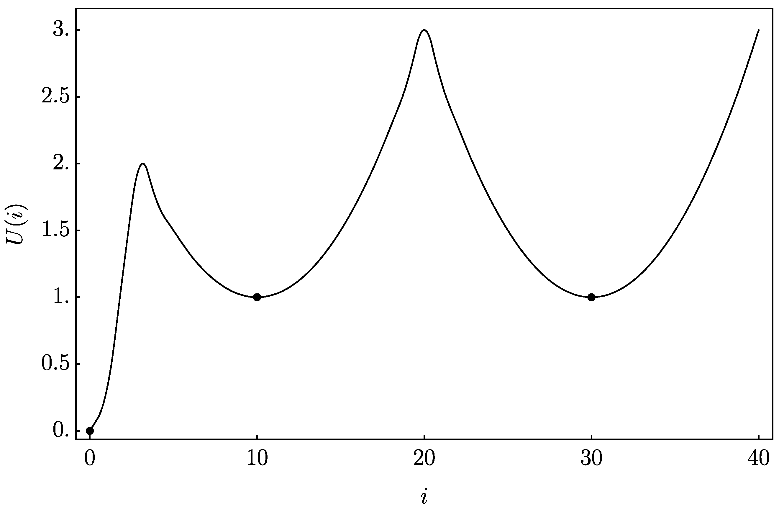
Let us consider a one-step chain $\mathcal{S}=\{0,1,\dots ,40\}$ with reflecting right boundary (${\lambda }_{40}=0$), attempt frequency $\nu =1$, and inverse temperature $\beta =5$. The piecewise-quadratic potential (see Figure 1)

$$U\left(i\right)=min\{0.3i^2,0.02{(i-10)}^2+1,0.02{(i-30)}^2+1\}$$

(36)

is used, which creates two wells at $i=10$ and $i=30$ and a half-well adjacent to the absorbing extinction state at $i=0$, separated by two barriers. Rates follow the local-symmetric mapping in Equation (2), which enforces detailed balance for this numerical example; the corridor and renewal formulas used below require only the one-step birth–death structure.

Here focus is on the corridor $[L,R]=[10,30]$ and on extinction from $L^{-}=10$ on $[0,10]$. The intrawell basins used below are single-site ($a=L$ or $c=R$) and one-sided basin with caps $a=0$ and $c=40$.

From Equations (3)–(5), $w,s,e$ are computed, then from Equations (11), (25) and (26) the attempt success probability and attempt duration from $L+1$ are obtained:

$$q_{L+1}\approx 5.095\times {10}^{-5},T_{L+1}\approx 2.420.$$

For single-site intrawell waiting, using Equations (2) and (6), ${\Theta }_L=1/{\lambda }_L=\nu e^{\frac{\beta }{2}(U\left(11\right)-U\left(10\right))}\approx 1.0513$ and ${\Theta }_R=1/{\mu }_R=\nu e^{\frac{\beta }{2}(U\left(29\right)-U\left(30\right))}\approx 1.0513$. The macroscopic rates in Equation (23) are then

$$k_{10\to 30}\approx {\displaystyle \frac{5.094\times {10}^{-5}}{1.0513+2.420}}\approx 1.467\times {10}^{-5},k_{30\to 10}\approx 1.467\times {10}^{-5}.$$

Both rates are nearly equal due to the symmetry of the wells at $n=10$ and $n=30$ in this example.

If instead one-sided basin intrawell models are adopted via Equations (16) and (17) (with $a=0$, $c=40$), one obtains ${\Theta }_L\approx 3.372$ and ${\Theta }_R\approx 3.470$, which reduces the effective rates accordingly. The corridor-only attempt rate (set $\Theta =0$) serves as an upper bound. The resulting basin-intrawell transition rates are

$$k_{10\to 30}\approx {\displaystyle \frac{5.094\times {10}^{-5}}{3.372+2.420}}\approx 8.794\times {10}^{-6},k_{30\to 10}\approx {\displaystyle \frac{5.094\times {10}^{-5}}{3.470+2.420}}\approx 8.648\times {10}^{-6}.$$

Let us now consider the extinction rate $k_{L^{-}\to 0}$ from the left well using both the single-site and one-sided basin intrawell models. In this example the leftmost metastable well is $L^{-}=10$ and extinction occurs through the corridor $[0,L^{-}]$, with absorbing endpoints at 0 and $L^{-}$. On this corridor, the scale–speed arrays $(w,s,e)$ are computed and the extinction is evaluated throughput formula in Equation (29). In addition to the corridor quantities $p_{\mathrm{succ}}$ and $T_{L^{-}-1}^{[0,L^{-}]}$, the renewal denominator requires the intrawell initiation time ${\Theta }_L^{-}$, which is the mean time to initiate a leftward attempt, i.e., to reach $L^{-}-1$ starting from $L^{-}$ while remaining in the right-side basin attached to the left well.

In the single-site model, ${\Theta }_L^{-}=1/{\mu }_{L^{-}}\approx 1.0513$, as mentioned earlier, and Equation (29) yields $k_{L^{-}\to 0}\approx 2.450\times {10}^{-3}$. For the one-sided basin model, the leftward initiation time must be computed using the right basin $[L^{-},c^{-}]$, because the attempt is initiated by moving left out of $L^{-}$ after wandering to the right within the basin. Therefore, ${\Theta }_L^{-}$ is evaluated using the one-sided series (Equation (17) with $R\mapsto L^{-}$) and the basin cap $c^{-}=20$ is chosen, i.e., the midpoint between the two wells. With this choice, $k_{L^{-}\to 0}\approx 1.432\times {10}^{-3}$ is obtained. Thus, incorporating intrawell sojourn within the basin reduces the predicted extinction rate by approximately $42\%$. This reduction is an order-one effect: it enters only through the renewal denominator ${\Theta }_L^{-}+T_{L^{-}-1}^{[0,L^{-}]}$ and propagates directly to the coarse-grained mean extinction times reported below. The estimated microscopic and coarse-grained quantities for the two intrawell models are summarized in

Table 1. Results for the double-well example with single-site intrawell waiting times.

Quantity	Notation	Value
Success probability	$q_{L+1}$	$5.094\times {10}^{-5}$
MFPT	$T_{L+1}$	$2.420$
Success probability	$q_{R-1}$	$0.9999$
MFPT	$T_{R-1}$	$2.420$
Intrawell (left)	${\Theta }_L$	≈1.0513
Intrawell (right)	${\Theta }_R$	≈1.0513
Rate $10\to 30$	$k_{L\to R}$	$1.467\times {10}^{-5}$
Rate $30\to 10$	$k_{R\to L}$	$1.457\times {10}^{-5}$
Extinction rate	$k_{L^{-}\to 0}$	$2.450\times {10}^{-3}$

and

Table 2. Results for the double-well example with one-sided basin intrawell waiting times.

Quantity	Notation	Value
Success probability	$q_{L+1}$	$5.095\times {10}^{-5}$
MFPT	$T_{L+1}$	$2.420$
Success probability	$q_{R-1}$	$0.9999$
MFPT	$T_{R-1}$	$2.420$
Intrawell (left)	${\Theta }_L$	≈3.372
Intrawell (right)	${\Theta }_R$	≈3.470
Rate $10\to 30$	$k_{L\to R}$	$8.794\times {10}^{-6}$
Rate $30\to 10$	$k_{R\to L}$	$8.648\times {10}^{-6}$
Extinction rate	$k_{L^{-}\to 0}$	$1.432\times {10}^{-3}$

.

Using the coarse-grained method of Section 6, the MTE is computed starting from each well. The resulting MTEs for initial wells $L=10$ and $R=30$ are reported in

Table 3. Mean extinction time of metastable wells, showing comparison between the coarse-grained (CG) and exact values. The coarse-grained values are calculated using the single-site (SS) intrawell model (CG(SS)) and the one-sided basin intrawell model (CG(basin)).

MTE	CG(SS)	CG(basin)	Exact
$T_{30}^e$	69,450	117,040	117,066
$T_{10}^e$	816	1408	1405

. Let us validate these values by computing the exact MTE for the full one-step chain from the Kolmogorov backward equation for mean passage times [2,11]. The one-sided basin intrawell model yields MTEs that agree closely with the exact computation, whereas the single-site intrawell model underestimates the intrawell contribution $\Theta$ and consequently overestimates the effective coarse-grained rates $k=q/(\Theta +T)$, leading to systematic underestimation of MTEs.

7.1. Sensitivity to Basin-Cap Placement (Interface Choice) and Robustness of Coarse-Graining

Let us now provide a meaningful comparison between exact and coarse-grained predictions as model parameters vary, then provide a sensitivity analysis to identify the parameters which matter most. In the framework used here, a practically important and unavoidable modeling choice is the placement of basin caps that define the intrawell domains used to compute one-sided waiting times. Specifically, for a left well $W_1$, a left basin $[a,W_1]$ is used to compute ${\Theta }_{W_1}$; for a right well $W_2$, a right basin $[W_2,c]$ is used to compute ${\Theta }_{W_2}$; and for extinction from the leftmost well, a right cap $c^{-}$ is used to define the basin $[W_1,c^{-}]$ that controls the leftward initiation time ${\Theta }_{W_1}^{-}$. Varying these caps does not change the corridor committor q or the corridor attempt duration T, since the corridor endpoints remain fixed at the wells; however, it does change the renewal denominator $\Theta +T$, and hence the effective rates $k=q/(\Theta +T)$. Therefore, basin-cap sweeps provide a direct sensitivity probe of how intrawell sojourn affects extinction and switching.

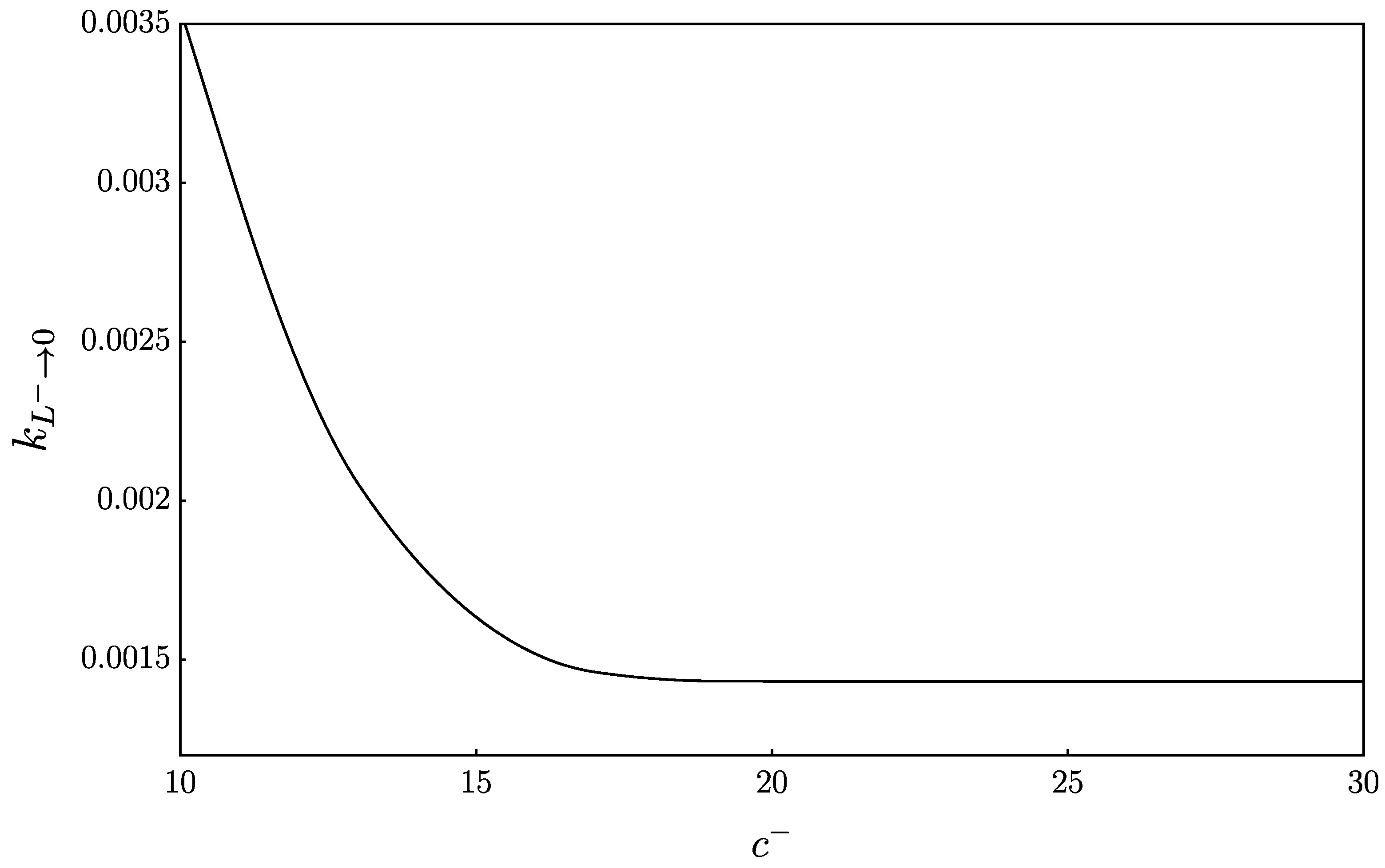
Let us begin with extinction from the left well. Figure 2 shows the extinction rate $k_{L^{-}\to 0}$ as a function of the right basin cap $c^{-}$ used in $[W_1,c^{-}]$ for the one-sided extinction initiation time ${\Theta }_{W_1}^{-}$. As $c^{-}$ increases, the basin widens and the chain spends a longer time wandering before making a successful leftward excursion to the absorbing state; correspondingly, $k_{L^{-}\to 0}$ decrease, then saturates once $c^{-}$ lies beyond the barrier region separating the two wells. This monotone decrease is the quantitative expression of the statement that intrawell residence times can produce an order-one correction to extinction rates.

Next, let us quantify how basin-cap placement impacts the coarse-grained prediction of mean time to extinction (MTE). We measure accuracy via the relative error

$$\mathrm{Relative}\mathrm{Error}\left(T_{W_i}^e\right)={\displaystyle \frac{T_{W_i}^{e,\mathrm{CG}}-T_{W_i}^{e,\mathrm{Exact}}}{T_{W_i}^{e,\mathrm{Exact}}}},$$

(37)

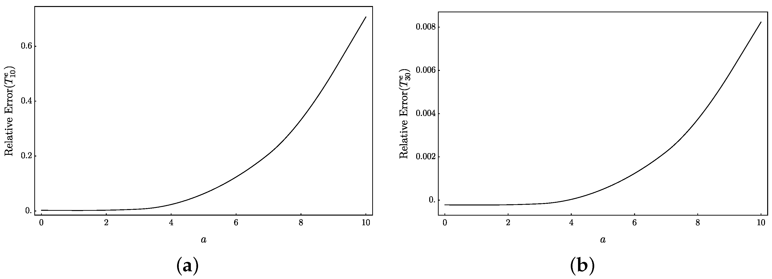
where $T_{W_i}^{e,\mathrm{CG}}$ is the MTE produced by the coarse-grained generator with one-sided basin rates and $T_{W_i}^{e,\mathrm{Exact}}$ is the exact MTE from the full microscopic backward equation. Figure 3a,b shows $\mathrm{Relative}\mathrm{Error}\left(T_{10}^e\right)$ and $\mathrm{Relative}\mathrm{Error}\left(T_{30}^e\right)$ as the left basin cap a is varied in $[a,W_1]$ (with the other caps fixed). The error for $T_{10}^e$ grows rapidly as a approaches $W_1$, reflecting the fact that shrinking $[a,W_1]$ forces ${\Theta }_{W_1}$ toward the single-site limit, thereby overestimating the escape and extinction rates from the left well. In contrast, the error in $T_{30}^e$ remains much smaller over the same sweep, indicating that for this parameter set the MTE starting from the right well is less sensitive to the left-basin truncation than the MTE starting from the left well.

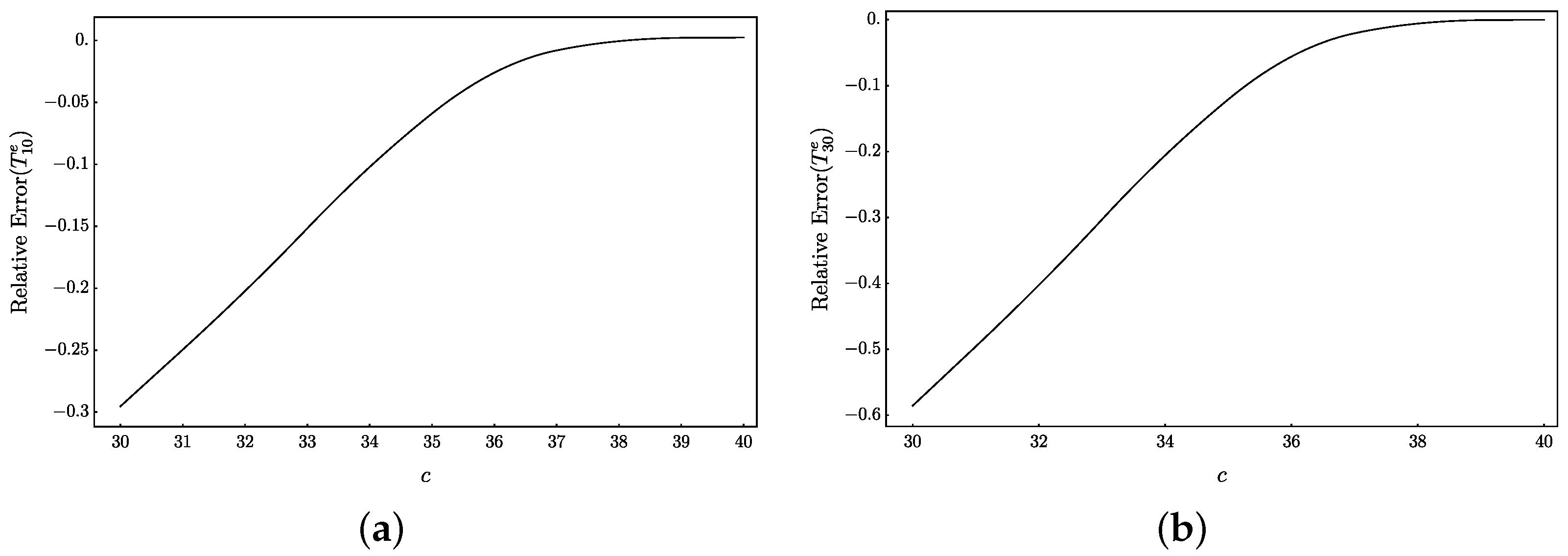
Figure 4a,b performs the complementary sweep in the right basin cap c for $[W_2,c]$ while holding the left cap fixed, plotting $\mathrm{Relative}\mathrm{Error}\left(T_{10}^e\right)$ and $\mathrm{Relative}\mathrm{Error}\left(T_{30}^e\right)$ as functions of c. Here, the relative error is negative for small c, which is consistent with an underestimated intrawell waiting time ${\Theta }_{W_2}$ and hence an overestimated return rate $k_{W_2\to W_1}$, which shortens the coarse-grained residence time in the right well and reduces the MTE. As c increases toward the physical boundary, ${\Theta }_{W_2}$ increases and the coarse-grained prediction converges toward the exact MTE. This sweep shows that for MTEs starting in the right well, accurate modeling of intrawell residence on the right side is essential; truncating $[W_2,c]$ too aggressively leads to an order-one underestimation of $T_{30}^e$, whereas sufficiently large c yields near-zero relative error.

Overall, the basin-cap sensitivity curves provide a practical diagnostic; when the relative error either plateaus under further increases of $c^{-}$ or c or decreases in a, the coarse-grained predictions are robust to basin placement; conversely, strong cap dependence indicates that intrawell residence dominates the renewal denominator $\Theta +T$ and cannot be neglected.

8. Results and Discussion

In this paper, a two-step approach have been adopted: solving the dynamics of each corridor at the microscopic level, followed by a coarse-grained well graph which yields a compact description of extinction in multi-metastable one-step chains. At the micro level, scale/speed identities provide closed forms for committors, mean first-passage times (MFPTs), and one-sided intrawell waiting times; a renewal–reward decomposition then turns these into effective well-to-well rates of the form $k=q/(\Theta +T)$ that separate (i) success probability along a corridor from (ii) the mean cycle duration (intrawell waiting plus corridor attempt time). At the macro level, these rates define a small CTMC on wells plus an absorbing extinction node for which mean extinction times (MTEs) and pre-extinction residence times follow from the standard transient-chain linear system $(-Q_T){\mathbb{T}}^e=\mathbf{1}$ and its fundamental matrix ${(-Q_T)}^{-1}$. This pipeline preserves finite-n discreteness and does not require a small-noise or continuum limit (contrast with the Kramers/WKB methods) [1,6,20,29].

Concretely, in the worked example (double-well with absorbing 0), the corridor series produce success probabilities q, attempt durations (MFPTs) T, and intrawell means $\Theta$, which combine into renewal rates $k=q/(\Theta +T)$. Plugging these into the coarse generator reproduces MTEs that match exact backward-equation values to high accuracy when one-sided basin intrawell series are used (see Table 3). For $W_2=30$, the coarse-grained (basin) and exact MTEs differ by less than $3\times {10}^{-4}$ relative error, and for $W_1=10$ by less than $3\times {10}^{-3}$. By contrast, the single-site intrawell model substantially overestimates effective rates (and hence underestimates MTEs), quantifying the practical importance of intrawell waiting (Table 3).

A further practical outcome is that an internal sensitivity analysis with respect to basin definitions can be performed on the model. In many applications, basin caps $(a_k,c_k)$ for each well $W_k$ are not uniquely prescribed and must be chosen from physical considerations (for example, midpoints between wells, drift-reversal points, or geometric boundaries). Figure 2, Figure 3 and Figure 4 quantify how coarse-grained extinction observables vary under such choices for one sided basins. The key point is that cap dependence enters primarily through the intrawell terms $\Theta$ and ${\Theta }^{-}$, not through the corridor committors or corridor attempt durations; thus, the sensitivity plots directly diagnose whether intrawell residence dominates the renewal denominator $\Theta +T$. In the present example, $k_{L^{-}\to 0}$ decreases and saturates as $c^{-}$ increases (Figure 2), showing convergence once the left-well basin extends beyond the barrier region. Likewise, the relative-error sweeps in a and c (Figure 3 and Figure 4) identify which intrawell domain is the limiting source of coarse-grained error: aggressive truncation of $[a,W_1]$ produces large error in $T_{10}^e$, while aggressive truncation of $[W_2,c]$ produces order-one underestimation of $T_{30}^e$. This provides a basis for how to choose basis in practice: increase caps until the predicted MTEs (or their relative errors) plateau, at which point the coarse-grained estimates are robust.

Coarse-graining helps to illuminate the route to extinction. Exact one-step formulas for MTEs compress all pathways into a single scalar; they are elegant, but less transparent about how extinction occurs. The two-step reduction used here preserves a path decomposition: each edge rate encodes a specific corridor route through the product of a success probability and a mean cycle duration, while the fundamental matrix decomposes the total time into pre-extinction residence times per well (Section 6; see also Equations (33)–(35) for the $m=2,3$ cases). This yields distict controls; changing barriers affects q and T, whereas reshaping basins affects $\Theta$.

Let us now discuss the mapping of discrete states to physical systems such as ion channels or gene regulation and calibrating the local rates ${\lambda }_i,{\mu }_i$. The discrete one-step framework is intended to be instantiated directly from either (i) measured neighbor-to-neighbor transition statistics or (ii) a mechanistic rule that supplies local rates. To apply the theory, one first chooses a discrete state coordinate i that captures the slow metastable progression (for example, a small integer activation count, a cluster size, or a molecule number). The microscopic model is then fully specified by the adjacent rates $\{{\lambda }_i,{\mu }_i\}$ in the generator (1), which can be obtained in two common ways.

(a) Empirical (data-driven) local rates. If time series data of the discrete state are available, one may estimate ${\lambda }_i$ and ${\mu }_i$ from observed counts of $i\to i+1$ and $i\to i-1$ transitions together with state-resolved holding times (consistent with exponential waiting at each i in a CTMC). This is the most direct route in ion channel gating models and other Markov state descriptions, where transition intensities between neighboring conductance/activation levels are inferred from dwell time statistics. For instance, if i denotes the number of activated subunits (out of M), a standard nearest-neighbor closure is

$${\lambda }_i=(M-i)\alpha ,{\mu }_i=i\beta ,$$

where $\alpha$ and $\beta$ are elementary activation/deactivation rates (often voltage- or ligand-dependent). In this interpretation, wells correspond to long-lived closed/open macrostates, while extinction (state 0) can represent irreversible inactivation or loss of conducting subunits.

(b) Mechanistic local rates from an effective landscape. When an effective discrete potential or free-energy profile $U\left(i\right)$ is available (from equilibrium sampling, umbrella sampling, or a coarse thermodynamic model), one may use a local-symmetric rule such as Equation (2) to assign adjacent rates. This preserves detailed balance for equilibrium landscapes while still feeding into the same corridor and renewal objects $(q,T,\Theta )$ used in the coarse-grained rates.

In population and gene regulation settings, a natural choice is to take i as a copy number. A common birth–death structure is a nonlinear production rate ${\lambda }_i$ (for example, due to feedback or saturation) together with an approximately linear loss ${\mu }_i\propto i$ (degradation or death). In such models, extinction corresponds to $i=0$ exactly (not a continuum boundary layer), and the present coarse-grained reduction summarizes long-lived expression states (wells) and the rare transitions between them via locally computed corridor statistics.

Finally, the basin definitions used for intrawell times admit an operational interpretation in data-driven applications; basin caps correspond to the intrawell domain over which the system equilibrates rapidly before launching a corridor attempt. Thus, once local rates are specified, the sensitivity curves in Section 7.1 provide a practical diagnostic for model construction: if predicted observables vary strongly with basin caps, then intrawell residence dominates $\Theta$ and must be modeled with comparable fidelity.

Let us now discuss the role of heterogenous transition rates dependent on each state in relation to the homogeneous(constant) rates independent of the state. In some applications, the adjacent transition rates fluctuate only weakly around constants, for example, ${\lambda }_i=\overline{\lambda }(1+{ϵ}_i)$ and ${\mu }_i=\overline{\mu }(1+{\delta }_i)$ with $|{ϵ}_i|,|{\delta }_i|\ll 1$. In such cases, it is natural to ask whether the model can be simplified by replacing the full arrays with averaged rates $(\overline{\lambda },\overline{\mu })$. This can be adequate when the relevant corridor is short enough and fluctuations in the local bias ratio $r_i={\mu }_i/{\lambda }_i$ are quite small. However, because corridor committors and MTEs depend on products of $r_i$, even mild multiplicative variability can accumulate across long corridors and lead to an $\mathcal{O}\left(1\right)$ change in splitting probabilities and attempt durations. For this reason, we retain the general arrays $\left\{{\lambda }_i\right\}$ and $\left\{{\mu }_i\right\}$ so that both the microscopic calculations and the resulting coarse-grained predictions remain exact in homogeneous and heterogeneous regimes.

In terms of computational scalability, computing exact MTEs by solving backward equations on the full chain costs $\mathcal{O}\left(n\right)$ per right-hand side and becomes unwieldy as n grows or when many starting wells are queried. By contrast, themethod used here computes local corridor series (each $\mathcal{O}\left(\mathrm{span}\right)$, where span is the corridor length), then solves a relatively small linear system on m wells (tridiagonal, hence $\mathcal{O}\left(m\right)$). Thus, large-n systems reduce to a comparably small discrete model without invoking a diffusion limit, maintaining integer states and an explicit absorbing state 0.

Where WKB methods excel asymptotically, the discrete series remain non-asymptotic and stable even with strong drift and finite barriers. In the example, the basin intrawell series align almost exactly with the full exact MTEs, while the single-site model provides an upper-rate (lower-time) bound which can serve as a conservative bracket in sensitivity checks.

The structure of the transition rates $k=q/(\Theta +T)$ reveals three distinct contributions that control mean extinction times.

• The success probability q reflects corridor bias and is suppressed by unfavorable scale ratios; in diffusion limits, it plays the role of Kramers-type exponential factors [1,6].
• The intrawell mean $\Theta$ captures basin breadth and local wandering. Large basins slow effective rates even when q is not exceptionally small; the one-sided series in Equations (16) and (17) quantify this contribution exactly.
• The attempt time T is the mean corridor residence time in a single attempt. It is additive in the renewal denominator, and can be subleading to $\Theta$ in broad basins but dominant in narrow ones.

This separation enables targeted interventions; to prolong persistence, one may increase $\Theta$ (widen/deepen basins) or decrease q (tilt barriers), whereas reversing these changes accelerates extinction. For extinction from the leftmost well, quasi-stationary viewpoints clarify pre-absorption residence behavior and prefactors [30].

Regarding the relationship to asymptotic theories, in smooth-potential and small-noise limits, the discrete scale/speed formulas collapse to Eyring–Kramers-type expressions, including prefactors determined by local curvatures [1,11]. For non-gradient drifts, action-based methods (GMAM/minimum-action) and irreversible Eyring–Kramers generalizations describe optimal escape paths and modified prefactors; the corridor rates considered provide a discrete counterpart that can be matched to (or used to calibrate) asymptotics at finite n [31,32,33].

To conclude, by reducing discrete birth–death dynamics to a coarse Markov chain on metastable wells, extinction times are obtained that are both interpretable and accurate at finite system sizes. The approach considered distinguishes the roles of barrier success, corridor times, and intrawell waiting while remaining computationally light compared to full-chain solvers, and can complement continuum asymptotic theories as well as data-driven coarse-graining approaches.