Article

Self-Similar Bridge Between Regular and Critical Regions

by
Vyacheslav I. Yukalov
1,2,*,
Elizaveta P. Yukalova
3 and
Didier Sornette
4,5
1
Bogolubov Laboratory of Theoretical Physics, Joint Institute for Nuclear Research, Dubna 141980, Russia
2
Instituto de Fisica de São Carlos, Universidade de São Paulo, CP 369, São Paulo 13560-970, Brazil
3
Laboratory of Information Technologies, Joint Institute for Nuclear Research, Dubna 141980, Russia
4
Institute of Risk Analysis, Prediction and Management (Risks-X), Southern University of Science and Technology, Shenzhen 518055, China
5
Swiss Finance Institute–Geneva, University of Geneva, 42, Bd du Pont d’Arve, CH 1211 Geneva, Switzerland
*
Author to whom correspondence should be addressed.
Submission received: 5 February 2025 / Revised: 7 March 2025 / Accepted: 16 March 2025 / Published: 28 March 2025
(This article belongs to the Special Issue Complexity in High Energy and Statistical Physics)

Abstract

:
In statistical and nonlinear systems, two qualitatively distinct parameter regions are typically identified: the regular region, which is characterized by smooth behavior of key quantities; and the critical region, where these quantities exhibit singularities or strong fluctuations. Due to their starkly different properties, those regions are often perceived as being weakly related, if ever. However, here, we demonstrate that these regions are intimately connected, specifically showing how they have a relationship that can be explicitly revealed using self-similar approximation theory. The framework considered enables the prediction of observable quantities near the critical point based on information from the regular region, and vice versa. Remarkably, the method relies solely on asymptotic expansions with respect to a parameter, regardless of whether the expansion originates in the regular or critical region. The mathematical principles of self-similar theory remain consistent across both cases. We illustrate this consistency by extrapolating from the regular region to predict the existence, location, and critical indices of a critical point of an equation of state for a statistical system, even when no direct information about the critical region is available. Conversely, we explore extrapolation from the critical to the regular region in systems with discrete scale invariance, where log-periodic oscillations in observables introduce additional complexity. The findings provide insights and solutions applicable to diverse phenomena, including material fracture, stock market crashes, and earthquake forecasting.

1. Introduction

For statistical and nonlinear systems exhibiting critical phenomena, two fundamentally distinct regions of their characteristic parameters are generally recognized. The first is the region where the system displays smooth behavior of its observable quantities. The second is the critical region, which is characterized by sharp variations in certain observable quantities, and it is often accompanied by oscillations and singular points. Due to these contrasting behaviors, those regions often appear unrelated, making it seem impossible to predict the behavior in one region based on knowledge of the other.
This paper argues that the regular and critical regions are deeply interconnected. When analyzing a specific observable quantity, let us remember that it retains the same defining properties across all values of the variable or parameter in question. These properties might be prominently exhibited in one region while remaining hidden, yet still present, in the other.
Critical phenomena are marked by scale invariance, which dictates the asymptotic behavior of the studied quantities in the critical region [1,2,3,4,5,6]. Typically, the behavior of observables in these regions is described by renormalization group equations, which leads to power law behavior as a specific case of continuous real-valued scaling [7,8,9,10,11,12,13,14]. However, observables far outside the critical point may retain scaling properties, albeit in a hidden form.
Similarly, critical phenomena associated with discrete scaling involve complex critical exponents, whose observable signatures manifest as log-periodic oscillations superimposed on the leading power law behavior [5,15]. These oscillatory features may persist beyond the critical point, though those features might not be readily apparent.
The possibility of log-periodic oscillations was mentioned by Theodore Harris [16]. In his study devoted to the theory of branching processes, Harris suggested that iterating a discrete mapping might yield log-periodic oscillations. The significance of discrete scale invariance lies in its broad applicability across various phenomena, including phase transitions and temporal critical phenomena with finite-time singularities. Discrete scale invariance, along with its characteristic log-periodic oscillations, has been documented in numerous contexts, such as in models defined on hierarchical lattices [17,18,19,20,21,22,23]; models on fractal structures [24,25,26,27,28,29,30] or on aperiodic structures with a fractal spectrum [31,32,33,34]; earthquake physics [35,36]; material fractures [37,38,39,40,41]; financial bubbles [42,43,44,45,46,47,48,49,50,51,52,53,54,55,56,57,58,59,60]; and different other systems [15,61,62,63,64,65,66,67,68,69,70,71,72,73]. Consequently, the derived solutions connecting regular and critical regions have wide-ranging applicability.
Methodologically, the bridge between the regular and critical regions is constructed using self-similar approximation theory, which has been recently reviewed in Refs. [13,74] (see also [75,76]). This approach allows for the extrapolation of an observable quantity from one region to another, using only an asymptotic expansion that is available in one region. For instance, starting with an asymptotic expansion for small values of a variable x 0 , the behavior of the observable at finite and even large values of x (including x ) can be determined. This is achieved by extracting the self-similar properties of the expansion terms and extending this self-similarity to other regions.
From a mathematical standpoint, it makes no difference whether the initial expansion is derived in the regular or the critical region, because a suitable change in variables allows one to transition from small to finite or large values. What indeed matters is the overall quality of the expansion—namely how many terms are included and how well those terms are defined.
This paper is organized as follows. In Section 2, to strengthen the completeness and persuasiveness of this paper, we first outline the fundamental principles of self-similar approximation theory and then describe the steps taken to perform the extrapolation. Section 3 offers an explicit example that verifies the capability of self-similar approximation theory to bridge the regular and critical regions for the equation of state of a statistical system. This example illustrates that, even starting from a regular region far removed from the critical point and even without prior knowledge of its existence, the theory delivers accurate quantitative predictions for both the location of the critical point and the associated critical exponent. Section 4 presents the construction of a bridge extrapolating the process that links the critical region of a system, exhibiting discrete scale invariance, with its regular region. Finally, Section 5 outlines the conclusions.

2. Self-Similar Approximation Theory

The method employed here for extrapolating asymptotic expansions from one region of the variable to another is based on the self-similar approximation theory. Naturally, it is not necessary to repeat the full mathematical foundation of the theory here as it has been extensively detailed in several papers and reviews [13,74]. However, it is helpful to briefly revisit the core concepts of the theory in order that it is understood why the self-similar approach can successfully extrapolate asymptotic expansions and bridge different regions with such seemingly diverse behavior.
Suppose one is interested in a real function f ( x ) of a real variable x 0 , which is not known explicitly but its k-th order expansion f k ( x ) is possible being expressed in powers of x and valid in the region, where x 0 ; then, one needs to extrapolate this asymptotic expansion to the region of a finite variable x. This can be conducted by means of the self-similar approximation theory, whose main points are sketched just below. We give only the basic ideas, and the detailed mathematical description can be found in the reviews [13,74].
  • Implantation of control parameters. The given asymptotic series, represented by the truncated expansion f k ( x ) , is typically divergent. To improve its convergence properties, we introduce control parameters u to obtain an expanded form F k ( x , u ) . These control parameters can be incorporated in various ways, including through initial conditions, variable transformations, or series transformations. This incorporation induces the convergence behavior of the series in subsequent steps.
  • Fractal transformation technique. An efficient method of implanting control parameters is through the fractal transform
    F k ( x , { n j } ) = j = 1 k x n j ( 1 + b j x ) ,
    where n j and b j are control parameters to be defined from training conditions.
  • Determination of control functions. To induce the convergence of the series { F k ( x , u ) } , the control parameters, in general, have to become control functions u k ( x ) , which are defined by optimization conditions, such as the minimization of a cost functional, or training conditions so that the sequence { F k ( x , u k ( x ) ) } be convergent.
  • Construction of an approximation cascade. The transition from an expanded form F k to the next expanded form F k + 1 can be interpreted as the temporal motion within a functional space in discrete time, which is represented by the approximation order k. The series { F k ( x , u k ( x ) ) } can be reformulated as a trajectory { y k ( f ) } of a dynamical system in discrete time, which is called a cascade. The evolution equation of the approximation cascade, in the vicinity of a fixed point, is given by the self-similar relation y k + p ( f ) = y k ( y p ( f ) ) .
  • Embedding of a cascade into flow. In order to pass from discrete time to continuous time, the approximation cascade can be embedded into the approximation flow, whose trajectory passes through all points of the cascade trajectory, and the evolution equation satisfies the self-similar relation y ( t + t , f ) = y ( t , ( y ( t , f ) ) .
  • Integration of an evolution equation. The self-similar relation can be reformulated as a Lie differential equation, which can then be integrated and analyzed to define fixed-point solutions. These solutions serve as the effective limit f k * ( x ) for the approximation sequence. The effective limit f k * ( x ) , representing a fixed point, is termed a self-similar approximant of order k.
Let the small-variable expansion with respect to x > 0 be
f k ( x ) = n = 0 k a n x n ( x 0 ) ,
where a 0 0 . And we want to extrapolate this expansion to finite values of x, and possibly to large values. Self-similar approximants, derived using the aforementioned procedure, are found to have the form of the factor approximants
f k * ( x ) = a 0 j = 1 N k ( 1 + A j x ) n j ,
where
N k = k / 2 , k = 2 , 4 , , ( k + 1 ) / 2 . k = 3 , 4 , ,
while A j and n j are the control parameters defined by the training conditions
lim x 0 1 n ! d n d x n f k * ( x ) = a n .
The function f k * ( x ) possesses a critical point x c if there exists m ( 0 , k ] for which
A m = min j A j < 0 and n m < 0 ,
so that 1 + A m x c = 0 , and the function f k * ( x ) exhibits divergence at x = x c . In the critical region, the function f k * ( x ) has the form
f k * ( x ) C k ( x c x ) α ,
with the critical point and critical exponent given by
x c = 1 | A m | , α = | n m | ,
the coefficient C k being
C k = a 0 j m N k ( 1 + A j x c ) n j .
Note that, if an expansion with respect to large variables, for example, z 1 , is given, then it can be straightforwardly transformed to an expansion over small variables by means of the variable change z = 1 / x .
A significant case that is often met is when the available information is minimal, where, for example, the expansion is
f ( x ) a 0 + a 1 x + a 2 x 2 ,
with nonzero a 0 and a 1 , while a 2 0 . The optimal self-similar approximant for the given minimal information can be determined by applying the approach described above to the truncated series (8), resulting in the self-similar factor approximant
f * ( x ) = a 0 ( 1 + A x ) n ,
where n is neither 0 nor 1. From the training conditions (3), n = a 1 / a 0 A 1 and A 1 0 . Taking into account that
lim A 0 ( 1 + A x ) 1 / A = e x ,
one obtains
f * ( x ) = a 0 exp a 1 a 0 x .
With additional expansion terms for f k ( x ) , more refined approximations for f k * ( x ) can be achieved, with higher-order terms providing higher accuracy. However, given the available minimal information, the best possible result is the extrapolation given by the approximant (10).
To conclude this Section, let us summarize the key insight of the self-similar approximation theory. Although perturbative series and their coefficients are typically derived for a specific region of a variable, those series inherently contain deeper information about the full function they approximate since the series are generated by that very function. The mathematical procedures outlined here allow us to uncover and leverage this hidden structure within asymptotic series. This explains, naturally, why self-similar approximation methods can effectively extrapolate results obtained in one domain of a variable to another, broader domain.
For practical applications of the theory to specific problems, it is not necessary to revisit the entire underlying methodology. Instead, the essential procedure is straightforward. Consider Expansion (1), which holds in the region of small values of the variable x that is looking for to extend to finite or even large values. The solution depends on the number of terms available in the given expansion (1). In the most simple case, when only a few terms are known, the approximant is given by Equation (10). As soon as more terms are available, the appropriate extrapolating form is the self-similar factor approximant (2), with parameters A j and n j determined by the training condition (3). This condition explicitly defines all parameters A j and n j . If these parameters satisfy condition (4), then a critical point exists, leading to approximant (5). This concise formulation encapsulates all what is required for the practical implementation of the general theory.

3. Bridging the Regular and Critical Regions for Statistical Systems

In statistical systems, reliable expansions are typically available for their regular regions, which are far from critical points, whereas the primary interest often lies in the understanding of the critical behavior. As a typical example, let us consider the equation of state for a fluid of hard discs of diameter σ . The equation of state is presented by the compressibility factor
Z = P ρ k B T ρ N disc V ,
where P denotes the pressure, ρ denotes the density, N disc and V represent the number of discs and the volume of the system, respectively, T is the temperature, and k B is the Boltzmann constant. By means of the perturbation theory, the compressibility factor can be found as an expansion in powers of density:
Z = 1 + 1 ρ n = 2 B n ρ n ( ρ 0 ) ,
where B n are the virial coefficients [77,78,79,80,81,82,83]. This expansion describes the regular region of asymptotically small density ρ 0 , which is located far outside of the critical region that is located near the closest packing density ρ c σ 2 = 2 / 3 = 1.1547 . The key question is whether it could be possible to predict the critical behavior of the fluid knowing only the asymptotic expansion (12) that is valid solely for the regular region far outside of the critical point of the closest packing density.
It is convenient to use dimensionless quantities expressing the compressibility factor as a function of the packing fraction:
x 1 2 ρ B 2 = π 4 ρ σ 2 .
Then, the asymptotic expansion (12) reads
Z k = 1 + n = 1 k b n x n ( x 0 ) ,
where the coefficients
b n = 2 n B n + 1 B 2 n
take the values
b 1 = 2 , b 2 = 3.1280 , b 3 = 4.2579 , b 4 = 5.3369 , b 5 = 6.3630 ,
b 6 = 7.3519 , b 7 = 8.3191 , b 8 = 9.2721 , b 9 = 10.2163 .
Summing up the expansion (14) by means of the self-similar approximation theory using the self-similar factor approximants [13,74,84,85,86], one finds the equation of state
Z k * = C k ( x c x ) α ,
where the coefficient C k converges to C = 1.54 for large enough k. The critical normalized density x c and the critical exponent α for different approximation orders k are given in Table 1. The critical point converges to x c = 0.99 and the critical exponent to α = 1.79 , which is in high agreement with the values obtained via numerical calculations [81].
Thus, the self-similar approximation theory not only enables connecting the critical region to the distant regular region, but it also provides precise quantitative predictions for the location of the critical point and the value of the critical exponent.

4. Bridging the Critical and Regular Regions for Systems with Discrete Scale Invariance

For systems with discrete scale invariance, the situation is the reverse to what was described in Section 3. There is quite a number of studies for the critical region but almost no information is available for the regular region. It is, therefore, necessary to start with the critical region and try to realize an extrapolation toward the regular region.
In the critical region, accomplishing the decimation procedure for lattice spin systems [8,10,12], it has been shown [17,87] that, in the vicinity of the phase transition point, the existence of discrete scale invariance leads to a specific renormalization group equation for the system free energy. The latter can be considered as a function of temperature, or of an effective coupling q = exp ( J / T ) , where J is a strength of spin interactions. Using the dimensionless relative coupling x = 1 q / q c , where q c = exp ( J / T c ) , with T c being a critical temperature, consider the decimation of scale λ > 1 and the related renormalization of x:
R ^ ( x ) = λ x , R ^ n ( x ) = λ n x .
The corresponding free energy per lattice site that has been shown in [17,87] to satisfy the equation
f ( x ) h 0 ( x ) + 1 μ f [ R ^ ( x ) ]
being related to the discrete scale invariance in the vicinity of the critical point, where x is close to zero and μ > 1 is the renormalization scale for the free energy. Equation (17) is only approximately valid near a critical point as each step of the decimation procedure typically involves the multiplication of effective couplings. The distinction between relevant and irrelevant couplings, which reduces their number, can only generally be made in the vicinity of a critical point [7,8,9,10,11,12,13,14].
By iterating Equation (17), one obtains a formal solution
f ( x ) n = 0 1 μ n h 0 [ R ^ n ( x ) ] .
The existence of discrete scale invariance is related to the occurrence of periodic or chaotic maps in the renormalization procedure [17].
It has been shown [88] that the free energy satisfying the renormalization group equations (17) and (18), connected with discrete scale invariance, can be represented as
f ( x ) h 0 ( x ) + x α n = 0 A n x i n ω ,
where α = ln μ / ln λ and ω = 2 π / ln λ . One can notice that using the identity
Re n = 0 A n x i n ω = n = B n x i n ω ,
where B 0 = A 0 and B n = B n = A n / 2 for n 1 , the free energy (19) can be rewritten in the form
f ( x ) h 0 ( x ) + x α n = B n x i n ω .
The appearance of complex powers leads to arising log-periodic oscillations, since
x i ω = cos ( ω ln x ) + i sin ( ω ln x ) .
In order to obtain complex powers, it is possible to work from the beginning in the complex plane, keeping in mind that the observable quantity is real. Assuming that, in the complex plane in the vicinity of a critical point, the observable satisfies the renormalization group equation, then we have
d F ( x ) d ln x G [ F ( x ) ] ,
where G [ F ( x ) ] is the Gell-Man–Low function [7,9,10,13,89,90], one can look for a solution by expanding the Gell-Man–Low function in powers of F ( x ) , as performed in Refs. [91,92,93,94,95].
In all cases, one obtains the behavior of observable quantities in the vicinity of a critical point, where discrete scale invariance is present. Here, the aim is to extrapolate the critical behavior to the regular region far outside the critical vicinity. Since there exist numerous phenomena exhibiting discrete scale invariance, one shall consider the behavior of their general typical representative denoted by a dimensionless function f ( x ) . We consider this characteristic quantity f ( x ) as a function of a dimensionless variable x. The quantity of interest can be a thermodynamic characteristic; an asset market price; a financial index; the intensity of acoustic emissions from a loaded material undergoing damage (or its amplitude of deformation); an electric current; or some other potential precursors of impending earthquakes. Without loss of generality, the function f ( x ) can be defined as being non-negative.
In the vicinity of a critical point x c , the studied quantity experiences a sharp increase. Depending on the considered particular case, the dimensionless variable x can represent relative pressure, relative elongation, relative temperature, relative effective coupling, relative time, or other relative parameters of the system:
x = 1 p p c , 1 l l c , 1 T T c , 1 q q c , or 1 t t c ,
respectively.
In that choice of variable, the initial point equals 1, while the critical point corresponds to zero:
x 0 = 1 , x c = 0 .
The choice (23) is convenient because then the critical region is characterized by x 1 , so that, in this region, it is possible to use expansions in powers of x. Thus, the introduced relative variable takes values in the interval
0 = x c x x 0 = 1 ,
while the normalized physical variable varies in the interval
0 = 1 x 0 1 x 1 x c = 1 .
An observable quantity I ( x ) can always be normalized, such as by defining f ( x ) = I ( x ) / I ( 0 ) , so that the dimensionless form for the function of interest is positive and satisfies the normalization
f ( 0 ) = 1 , f ( x ) 0 .
The aim here is to study the general case, when in the critical region in the vicinity of a critical point, there exists discrete scaling. Then, if so, in the critical region, the studied function f ( x ) can be represented as
f ( x ) 1 + g ( x ) ( x 0 ) ,
where g ( x ) is a function that, in the critical region, has the benefit of discrete scale invariance. When using the scale invariance relation, the representation (27) becomes equivalent to the expression (17). In view of the normalization condition f ( 0 ) = 1 , one gets the boundary condition
g ( 0 ) = 0 .
In order to find the general form of the considered function f ( x ) in the whole interval x [ 0 , 1 ] , from the knowledge of the existence in the critical region x 0 of discrete scaling, it is necessary to resort to the self-similar extrapolation procedure.
The function g ( x ) is assumed to satisfy a general type of scale invariance yielding complex exponents [5,15]. At the same time, it is not necessary to extend the consideration to the complex plane since complex exponents naturally appear after employing Fourier transformation.
The property of discrete scale invariance, arising in the vicinity of a critical point, reads
g ( λ x ) = μ g ( x ) .
Here, the scaling parameters λ > 1 and μ > 1 are assumed to be fixed. This is on the contrary to the continuous scaling, when these parameters are considered being arbitrary. Repeated use of the scaling relation yields
g ( λ n x ) = μ n g ( x ) ,
where the scaling parameters λ n = λ n and μ n = μ n compose a discrete spectrum with n = 0 , ± 1 , ± 2 , .
It is straightforward to check that the general solution of relation (29) has the form
g ( x ) = x α y ( x ) ,
in which, independently of n, we have
α ln μ ln λ ,
and the function y ( x ) can be expressed as
y ( x ) = F ln x ln λ ,
with F ( z ) being a periodic function of period 1:
F ( z + 1 ) = F ( z ) z ln x ln λ .
A periodic function can be expanded in the Fourier series as
F ( z ) = n = B n e i 2 π n z ,
which, using the notation of z in Equation (34), can be rewritten in the form
y ( x ) = n = B n e i n ω ln x ,
with the log-frequency
ω = 2 π ln λ .
The log-frequency ω encodes the existence of the preferred discrete scaling ratio λ , such that ln λ is the period of the oscillations in the ln x variable. Thus, λ is not a frequency (the inverse of time) in its natural sense but the preferred scaling factor. Keeping in mind a real function F ( z ) , hence real y ( x ) , gives the equality B n * = B n .
Thus, for the sought quantity (27) in the critical region, one has
f ( x ) 1 + x α y ( x ) , x 0 .
The expression (38) is only valid in the vicinity of a critical point, where x 0 . Therefore, it is possible to consider this expression as providing the first terms of an expansion
f ( x ) = m = 0 a m x m α y m ( x ) ,
where a 0 = a 1 = 1 .
A representation in the form of the infinite series (39) is not only merely inconvenient for practical use, but it also has several crucial deficiencies. Generally, such series are asymptotic and only have meaning in the limit x 0 . For a finite value of x, they not necessarily converge and even can become negative, breaking the condition of the semi-positiveness of f ( x ) . Dealing with such a series requires one to define its effective sum. This can be conducted by resorting to the self-similar approximation theory delineated in Section 2. In such a case, when just a few terms of an expansion is available and it is necessary to guarantee the semi-positiveness of the sought function, the method leads to approximant (10). This form guarantees the most suitable self-similar extrapolation under the minimally available information.
Note that, when more information becomes available, and the number of terms in an expansion is sufficiently large, it becomes possible to extend the form (10) by repeated iteration, leading to continued exponentials [96,97,98,99,100,101,102,103,104,105,106,107], which finds its justification [108] in self-similar approximation theory [13,74]. This type of exponential summation has been successfully applied to several problems [13,40,41,102,108,109,110,111,112,113].
Employing the self-similar approximant (10), the effective sum (39) can be represented by the expression
f ( x ) = exp { x α y ( x ) } .
As is stressed in this Section, the used approximation is based on the self-similar approximation theory that benefits from a sound mathematical foundation and has been demonstrated to provide an accurate approximations for a number of examples.
The coefficients B n in the expansion (35) are proportional to μ n < 1 what allows decreasing with n (see [17,88]). Keeping the first three terms, one has
F ( z ) = B 0 + B 1 e i 2 π z + B 1 * e i 2 π z ,
which yields
y ( x ) = a + b cos ( ω ln x ) c sin ( ω ln x ) ,
where
a = B 0 , b = 2 Re B 1 , c = 2 Im B 1 .
Equivalently, Equation (42) can be represented as
y ( x ) = a + b cos ( ω ln x + φ ) ,
with
φ = arctan c b = arctan Im B 1 Re B 1 .
In this way, the extrapolation of the studied observable quantity from the critical region, where x 0 , to arbitrary values of x reads
f ( x ) = exp { x α [ a + b cos ( ω ln x + φ ) ] } .
Note that setting b 0 corresponds to the case of continuous scale invariance, so that the function (44) reduces to
f 0 ( x ) = exp ( a x α ) .
The extrapolated function (44) represents the quantity of interest for all x in the domain [ 0 , 1 ] . In terms of physical behavior, one has to consider the variable 1 x for studying the behavior of the function f ( x ) from the initial point 1 x 0 = 0 to the critical point 1 x c = 1 .
In order to analyze the influence of discrete scale invariance, it is constructive to compare the full function f ( x ) with the case when only continuous scale invariance exists and discrete scale invariance is absent. This corresponds to the function (45). In the vicinity of the critical point, the continuous scale invariance leads to the power law in the exponential.
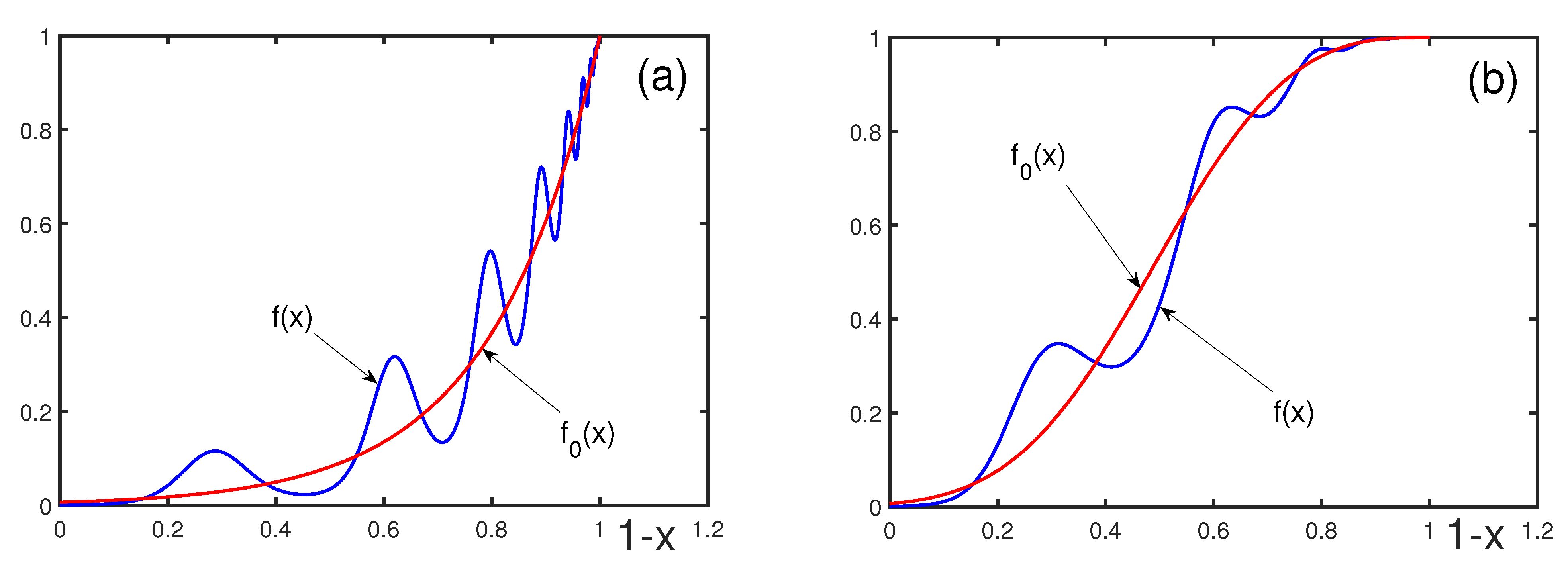
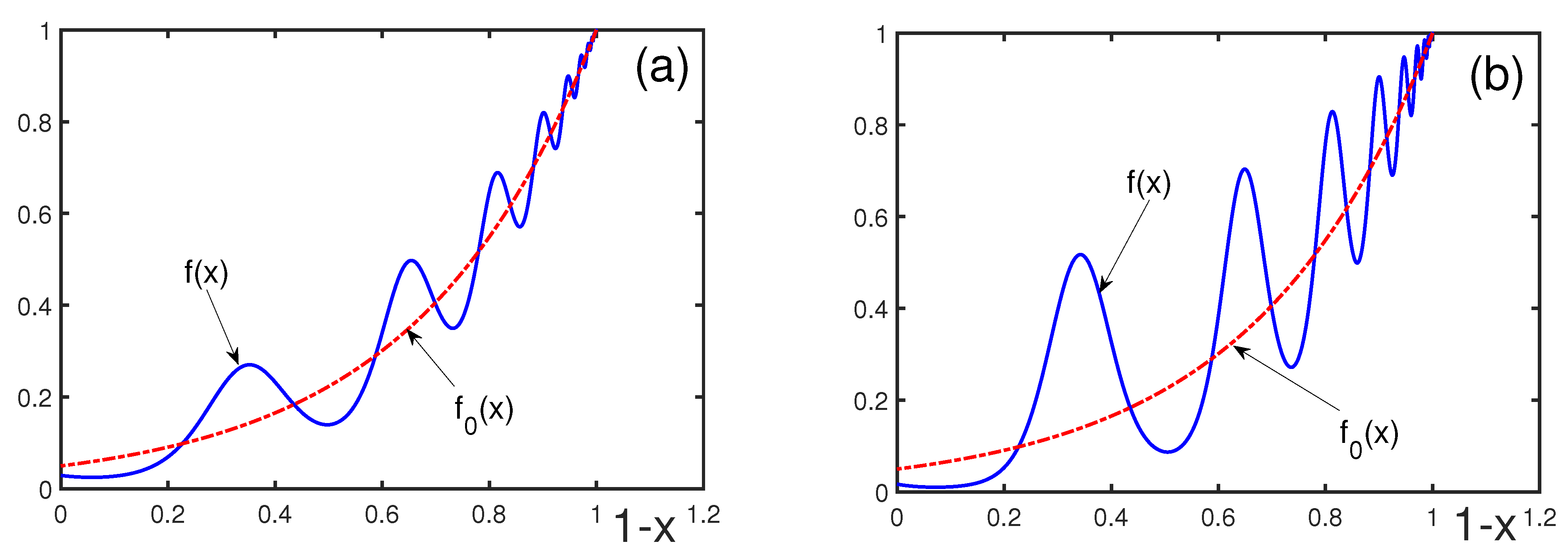
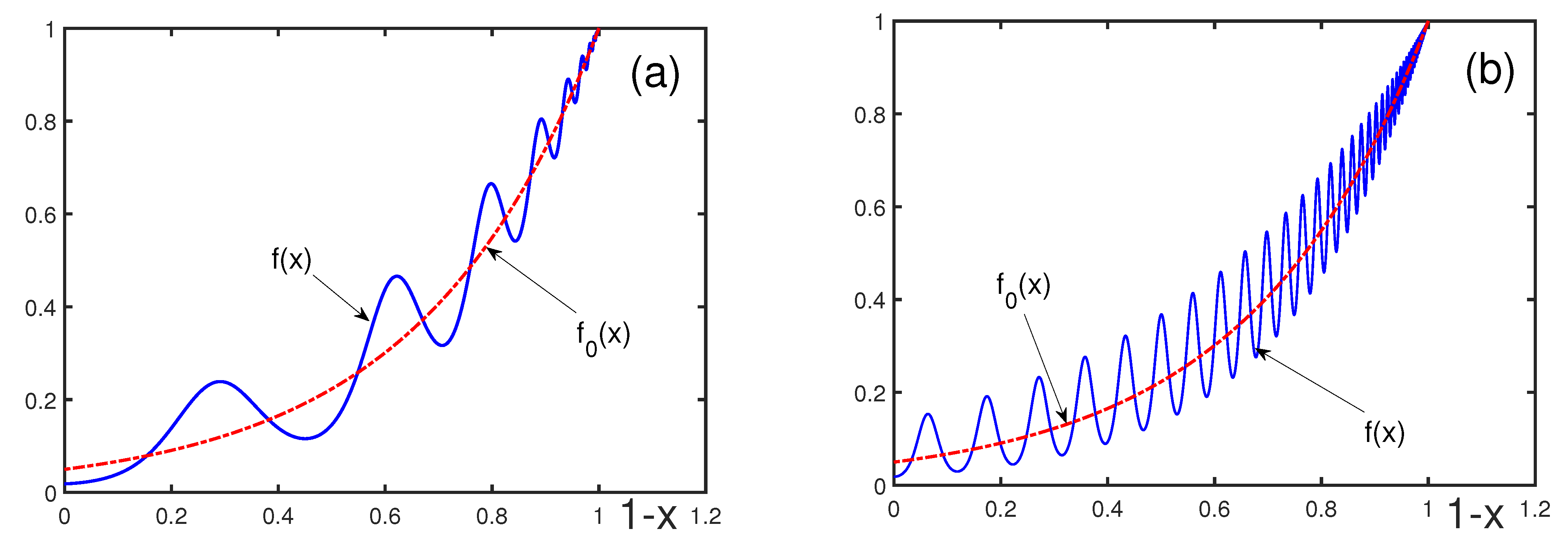
The typical behavior of f ( x ) , compared to f 0 ( x ) , as functions of 1 x , in the whole range [ 0 , 1 ] , is demonstrated in Figure 1, Figure 2, Figure 3, Figure 4 and Figure 5. The parameters are taken close to the values describing the behavior before material ruptures [39,40,41] and crashes in financial markets [43,44,45,46]. The role of the parameters entering f ( x ) is emphasized.
Figure 1 illustrates that the parameter ω controls the number of oscillations; the larger ω , the larger the number of oscillations. The phase shift φ , as is shown in Figure 2, moves the location of the oscillations, but it does not qualitatively change the overall picture. Increasing the parameter α smooths the log-periodic oscillations, and it makes f ( x ) larger, as can be found from Figure 3. Decreasing parameter a diminishes the oscillation amplitude, as shown in Figure 4. The absolute value of b influences the oscillation amplitude, making it larger by increasing | b | , as is evident from Figure 5.
The function F ( z ) , according to its representation (35), contains the modes with different frequencies. The reduction to the simplified form (41) is only valid when 1 / μ n 1 is for n > 1 , such that the coefficients B n quickly decrease with n and only the lowest mode is relevant.
In order to understand the influence of higher modes, it is necessary to study the behavior of the quantity (40) with the general form of the function
F ( z ) = B 0 + n = 1 B n e i 2 π n z + B n * e i 2 π n z ,
which leads to
y ( x ) = a + n = 1 b n cos ( n ω ln x + φ n ) ,
with b n = b / μ n 1 .
Note that, in Ref. [88], it was shown that two cases can happen: one is when the coefficients b n decrease exponentially as a function of n, such that only a few lower modes survive; and, the other case is when the coefficients b n decrease slower, such that many modes are to be taken into account. These two cases correspond to quite weak and strong log-periodicity, respectively. The form b n = b / μ n 1 , depending on the value of μ , can characterize these two cases. For μ > 1 , the coefficients decrease exponentially, and one can limit the consideration to a few first modes, while, for the μ close to 1, a number of modes to be taken into account, as is shown below.
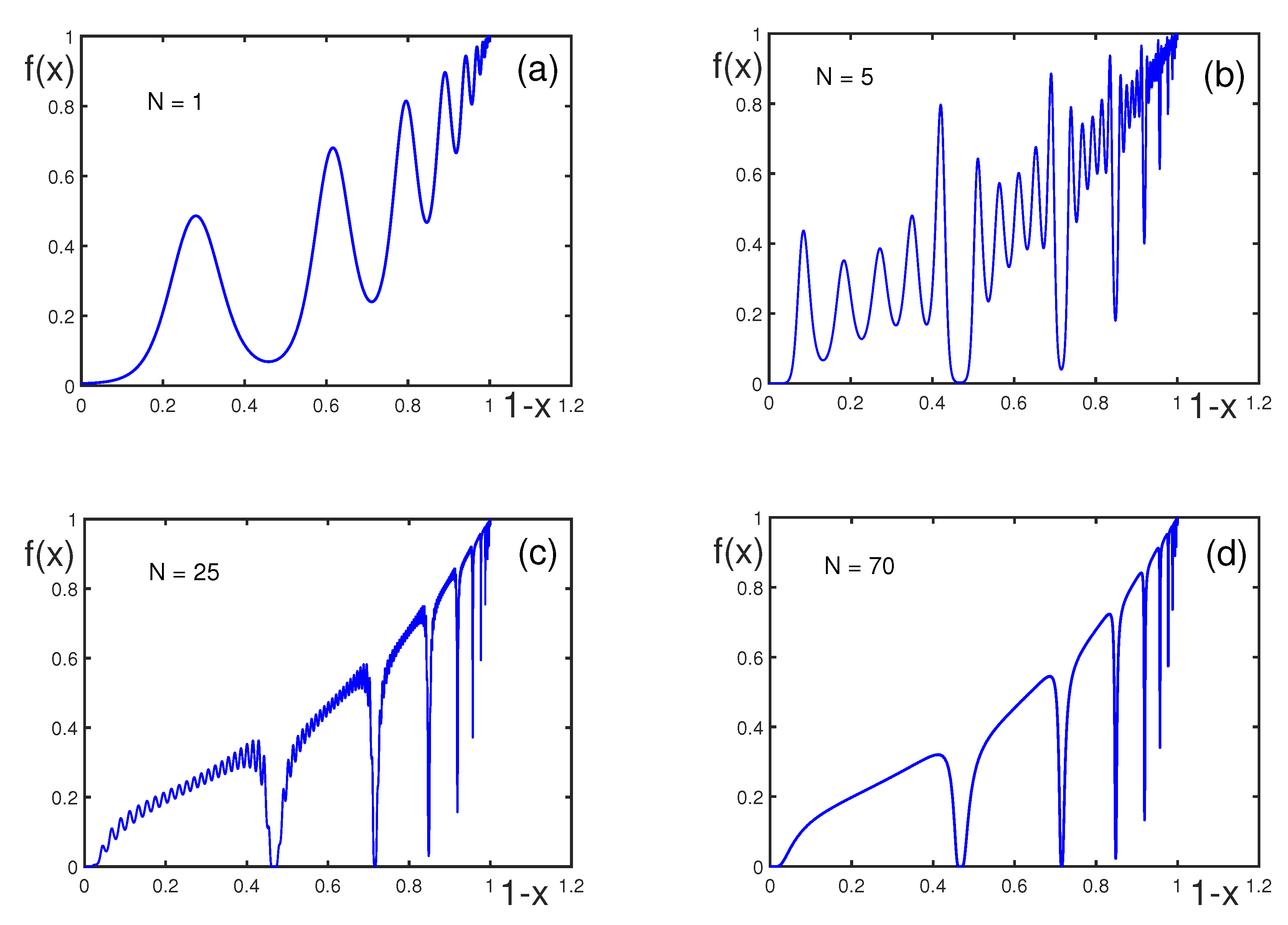
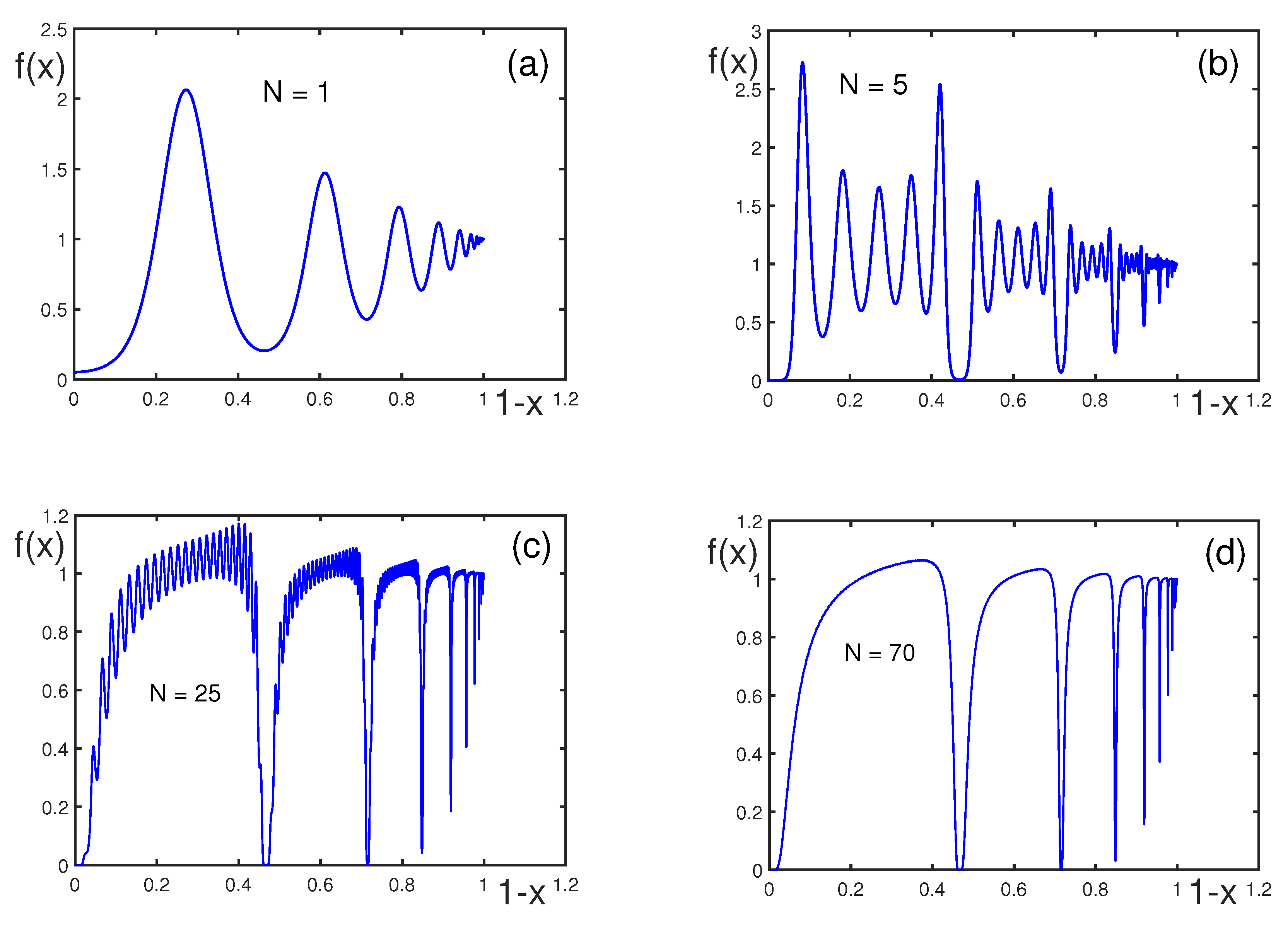
Figure 6 shows the typical behavior of f ( x ) , which is when the number N of modes increases until the function behavior ceases to change. The phases of all modes are assumed to be equal: φ n = φ . First, increasing the number of modes makes the oscillations more complex. When this number becomes close to N = 25 , a type of mode condensation occurs, which is characterized by shapes resembling deep troughs. Above N = 70 , the behavior of f ( x ) actually does not change (not shown). information in Figure 6, one finds that: (i) the log-periodic oscillations become increasingly complex with increasing number of modes N; (ii) a mode condensation effect starts as the number of modes reaches N = 25 ; and (iii) above N = 70 , the function stabilizes and does not change significantly, indicating that higher modes do not essentially affect the function.
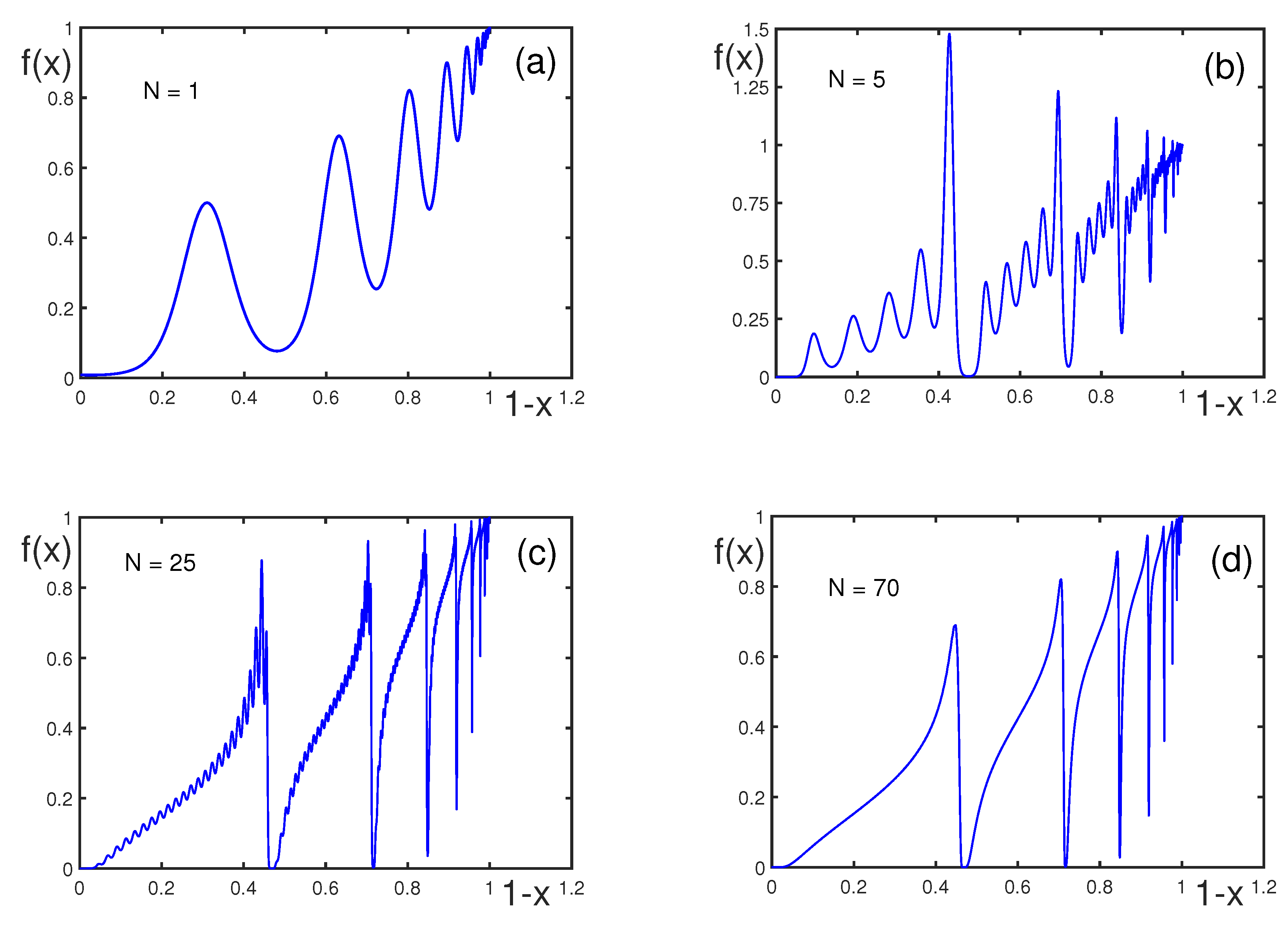
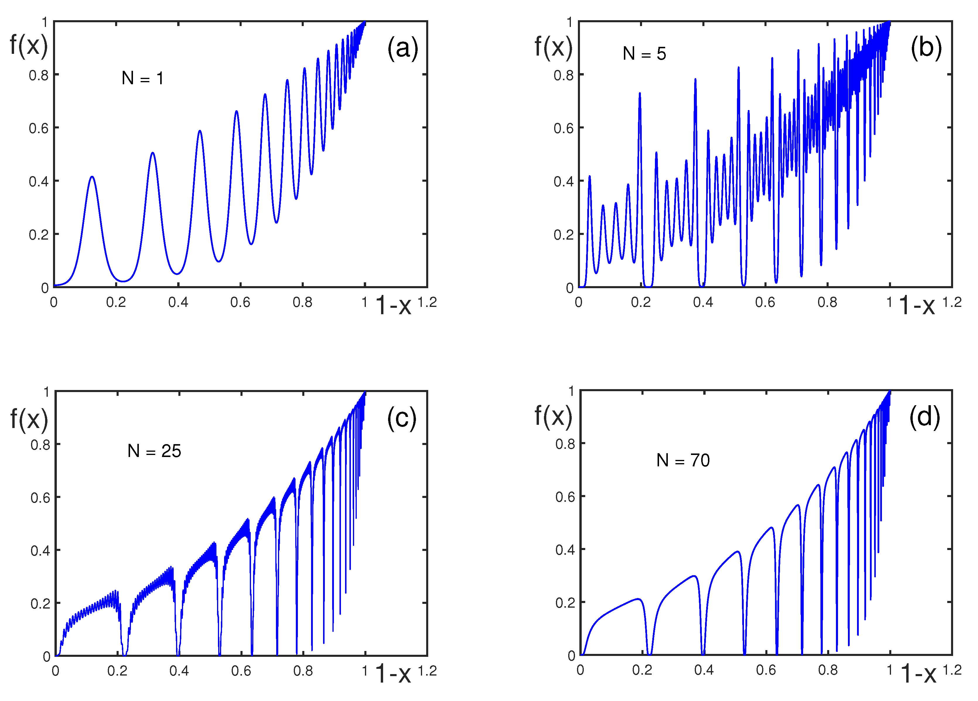
Varying the phase φ may result in the appearance of high peaks before the abrupt falls, as shown in Figure 7. The phase shift affects the alignment of oscillations. Overall, phase shift does not change the log-periodic structure of the oscillations much by merely relocating the oscillation peaks and slightly smoothing the latter. These variations may be productive in tuning models for specific applications, e.g., for the prediction of financial crashes or material rupture.
Decreasing the absolute value of negative a makes the peaks smoother, as shown in Figure 8, when compared with those shown in Figure 7. A smaller negative a suppresses the peaks and troughs compared to larger negative values. Again, as shown in Figure 7, the function stabilizes at N = 70 , which confirms that N = 70 is sufficient to capture full oscillation complexity.
The exponent α controls how quickly log-periodic oscillations grow. The smaller α = 0.3 , as shown in Figure 9, when compared with α = 1 in Figure 8, leads to smaller amplitudes of the oscillations and slower growth. The function is stable with respect to the increasing number of modes N above N = 70 (not shown), confirming the robustness of self-similar approximation.
The parameter ω controls the number of log-periodic oscillations. Figure 10 is plotted for larger ω , as compared to Figure 9, which results in more frequent oscillations. Influencing how densely spaced the oscillations are impacts how observable the log-periodic patterns appear in empirical data.
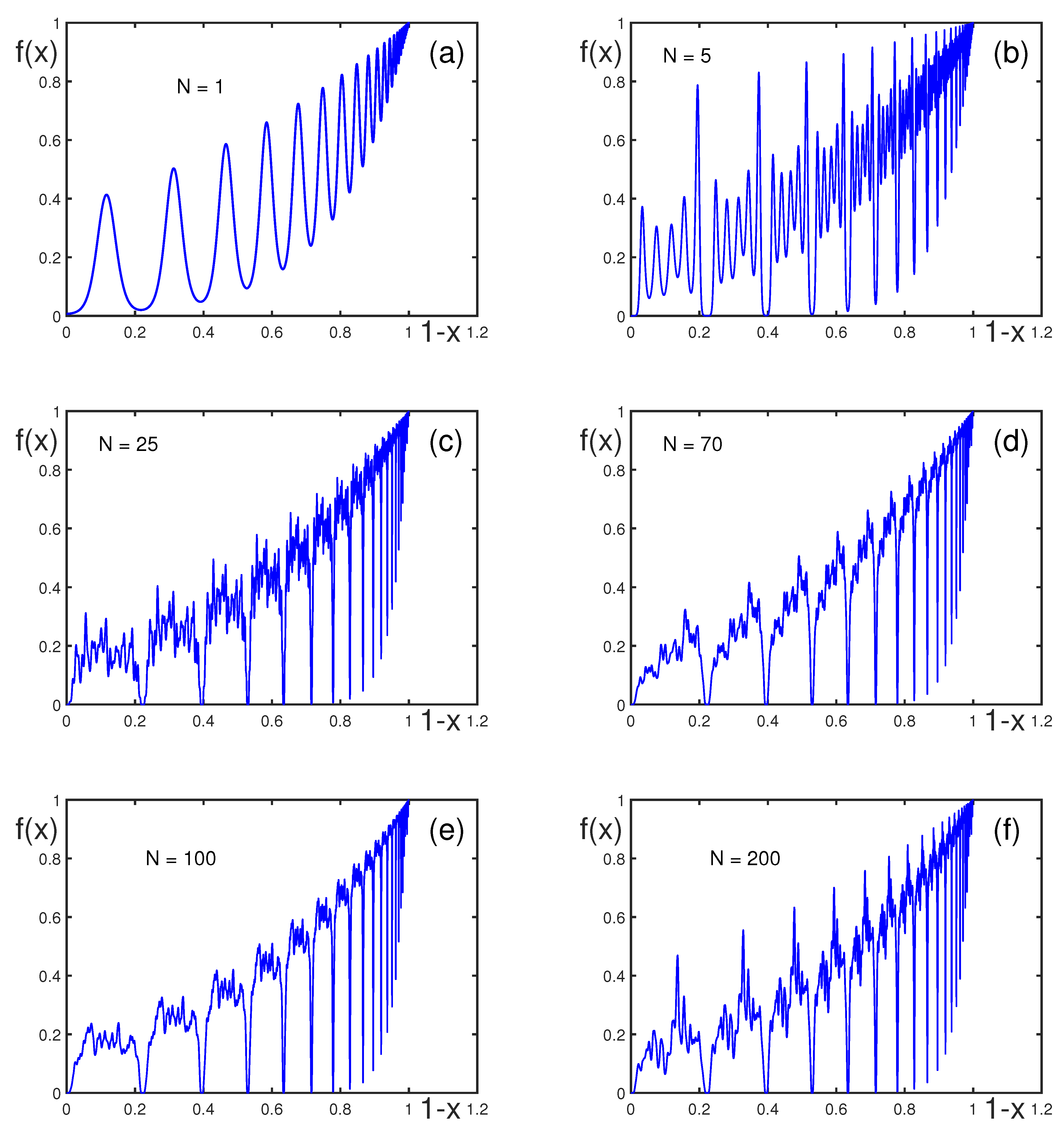
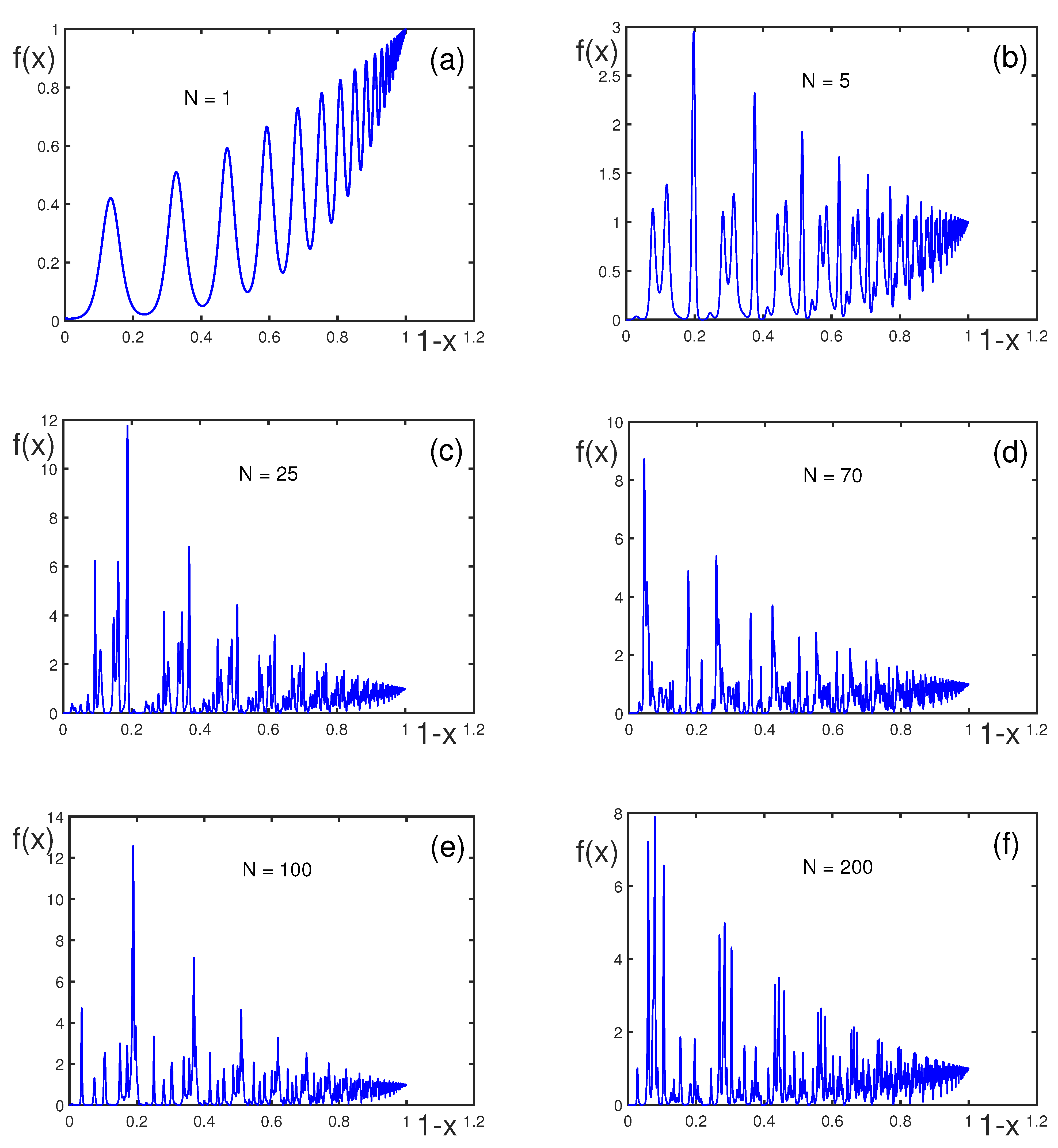
Figure 11 and Figure 12 demonstrate the influence of randomized phase effects on log-periodic oscillations. Random phases are drawn from normal distributions with different standard deviations. When phase values are randomized, the oscillations become ever chaotic. With an increasing number of modes, the N oscillations become increasingly irregular. For N > 25 , irregularity starts dominating, resembling a chaotic dynamic rather than a structured log-periodic pattern. Thus, randomness significantly affects the structure of fluctuations, with higher standard deviations leading to less predictable and more chaotic behavior. This picture is relevant for modeling natural phenomena, where oscillations are disrupted by random noise.
In conclusion, Figure 6, Figure 7, Figure 8, Figure 9, Figure 10, Figure 11 and Figure 12 explore how different parameters of the model influence log-periodic oscillations. When highlighting the key points, it is possible to summarize the following: (i) increasing the number of modes N enhances oscillation complexity; (ii) beyond the threshold N = 70 , further mode contributions become actually negligible; (iii) varying the phase shifts φ moves the oscillations but does not change their fundamental nature; (iv) the amplitude parameter a determines how pronounced the oscillations appear; (v) the exponent α governs the overall growth rate of oscillations; (vi) log-frequency ω directly influences how many oscillations appear over a given range; and (vii) phase randomness disturbs and can even destroy the standard picture of log-periodic oscillations, mimicking real-world systems where the main trends are often superimposed by random noise.

5. Conclusions

In this paper, we considered the relation between the regular region, which is far outside of a critical point and the critical region in the vicinity of the critical point in nonlinear systems. Despite the rather different behavior of the observable quantities in these regions, those regions are shown not being completely disconnected, but there is a bridge between them. We put forward the idea that the connection between the regular and critical regions can be recovered on the basis of self-similarity in the variation of their asymptotic forms in these regions. It is possible, starting with an asymptotic expansion in one of the regions, to explicitly extrapolate this expansion to another region. This can be accomplished employing the self-similar approximation theory, thus creating a self-similar bridge between the regions.
From a mathematical perspective, it is necessary to stress that it makes no difference whether the starting point is the regular region or the critical region. This is because what is necessary is the existence of an expansion in powers of some parameter. The theory allows for the extrapolation of any expansion, irrespectively of the nature of the parameter. Certainly, it is reasonable to start from the region where the expansion is better defined.
As an example of self-similar extrapolation from the regular to critical region, we considered a statistical system, which is represented by a fluid of hard disks. We have shown that, on the basis of an expansion in the regular region, being far outside the critical region and even having no information on its existence, it is straightforward to extrapolate the equation of state to the critical point; moreover, we have also shown that it is straightforward to predict the location of the critical point and to find the related critical exponent.
Another example studied here involves systems with discrete scale invariance. In this case, while more information is available on the system’s critical behavior, the regular region remains largely unexplored. This presents the challenge of extrapolating from the critical region to areas far beyond it. The issue is common across various critical phenomena exhibiting discrete scale invariance, such as earthquakes, material fractures, stock market crashes, and other “rupture” events.
A key conclusion to highlight is that log-periodic oscillations observed near a critical point do not emerge spontaneously. Rather, the oscillations are shown to exist well outside the critical region, though typically smaller in amplitude, less frequent, and smoother. This indicates that it is possible to identify and study log-periodic oscillations even at significant distances from the critical point. Furthermore, for certain parameter settings, these oscillations outside the critical region can exhibit quite large amplitudes. Varying the parameters can result in absolutely different behaviors, providing models for a wide range of processes, including the aforementioned earthquakes, material fractures, and stock market crashes.
The examples analyzed in this paper reinforce the concept that the regular and critical regions are profoundly interconnected. This relationship can be uncovered using self-similar approximation theory, which enables the construction of a self-similar bridge linking the regular and critical regions. This conclusion is broad in scope and applies to systems of various types and natures.

Author Contributions

All of the authors contributed to the study conception and design. Material preparation, data collection, and analysis were performed by V.I.Y., E.P.Y. and D.S. The first draft of the manuscript was written by V.I.Y., but all of the authors commented on previous versions of the manuscript. All authors have read and agreed to the published version of the manuscript.

Funding

D.S. was partially supported by the National Natural Science Foundation of China (Grant No. T2350710802 and No. U2039202), the Shenzhen Science and Technology Innovation Commission Project (Grants No. GJHZ20210705141805017 and No. K23405006), China, and the Center for Computational Science and Engineering at Southern University of Science and Technology, Shenzhen, China.

Data Availability Statement

No data are detailed in the manuscript.

Conflicts of Interest

The authors declare no conflicts of interest.

References

  1. Fisher, M.E. The Nature of Critical Points. In Lectures in Theoretical Physics, Volume VII C: Statistical Physics, Weak Interactions, Field Theory; Britin, W.E., Ed.; University of Colorado Press: Boulder, CO, USA, 1965; Available online: https://personal.rhul.ac.uk/UHAP/027/PH4211/PH4211_files/Fisher-1965.pdf (accessed on 15 March 2025).
  2. Brout, R. Phase Transitions; W.A. Benjamin, Inc.: New York, NY, USA, 1965. [Google Scholar]
  3. Stanley, H.E. Introduction to Phase Transitions and Critical Phenomena; Oxford University Press, Inc.: New York, NY, USA, 1987; Available online: https://archive.org/details/introductiontoph0000stan_h3y5/ (accessed on 15 March 2025).
  4. Yukalov, V.I.; Shumovsky, A.S. Lectures on Phase Transitions; World Scientific Co. Ltd.: Singapore, 1990. [Google Scholar] [CrossRef]
  5. Sornette, D. Critical Phenomena in Natural Sciences; Springer: Berlin/Heidelberg, Germany, 2006. [Google Scholar] [CrossRef]
  6. Quantum Statistical Mechanics:Selected Works of N.N. Bogolubov; Bogolubov, N.N., Jr., Ed.; World Scientific: Singapore, 2015. [Google Scholar] [CrossRef]
  7. Wilson, K.G.; Kogut, J. The renormalization group and the ε expansion. Phys. Rep. 1974, 12, 75–199. [Google Scholar] [CrossRef]
  8. Hu, B. Introduction to real-space renormalization group methods in critical and chaotic phenomena. Phys. Rep. 1982, 91, 233–295. [Google Scholar] [CrossRef]
  9. Bogoliubov, N.N.; Shirkov, D.V. Quantum Fields; Benjamin/Cummings Publishing Company, Inc.: Reading, MA, USA, 1983; Available online: https://www.scribd.com/doc/259563546/N-N-Bogoliubov-D-v-Shirkov-Quantum-Fields-BookFi-org (accessed on 15 March 2025).
  10. Kadanoff, L.P. Statistical Physics: Statics, Dynamics and Renormalization; World Scientific: Singapore, 2000. [Google Scholar] [CrossRef]
  11. Ma, S.-k. Modern Theory of Critical Phenomena; Routledge/Taylor & Francis Group: New York, NY, USA, 2009. [Google Scholar] [CrossRef]
  12. Efrati, E.; Wang, Z.; Kolan, A.; Kadanoff, L.P. Real-space renormalization in statistical mechanics. Rev. Mod. Phys. 2014, 86, 647–669. [Google Scholar] [CrossRef]
  13. Yukalov, V.I. Interplay between approximation theory and renormalization group. Phys. Part. Nucl. 2019, 50, 141–209. [Google Scholar] [CrossRef]
  14. Dupuis, N.; Canet, L.; Eichhorn, A.; Metzner, W.; Pawlowski, J.M.; Tissier, M.; Wschebor, N. The nonperturbative functional renormalization group and its applications. Phys. Rep. 2021, 910, 1–114. [Google Scholar] [CrossRef]
  15. Sornette, D. Discrete-scale invariance and complex dimensions. Phys. Rep. 1998, 297, 239–270. [Google Scholar] [CrossRef]
  16. Harris, T.E. Branching processes. Ann. Math. Stat. 1948, 19, 474–494. [Google Scholar] [CrossRef]
  17. Derrida, B.; Eckmann, J.-P.; Erzan, A. Renormalisation groups with periodic and aperiodic orbits. J. Phys. A Math. Gen. 1983, 16, 893–906. [Google Scholar] [CrossRef]
  18. Derrida, B.; De Seze, L.; Itzykson, C. Fractal structure of zeros in hierarchical models. J. Stat. Phys. 1983, 33, 559–569. [Google Scholar] [CrossRef]
  19. Derrida, B.; Itzykson, C.; Luck, J.M. Oscillatory critical amplitudes in hierarchical models. Comm. Math. Phys. 1984, 94, 115–132. [Google Scholar] [CrossRef]
  20. Bessis, D.; Geronimo, J.S.; Moussa, P. Mellin transforms associated with Julia sets and physical applications. J. Stat. Phys. 1984, 34, 75–110. [Google Scholar] [CrossRef]
  21. Itzykson, C.; Luck, J.M. Zeroes of the partition function for statistical models on regular and hierarchical lattices. In Critical Phenomena: 1983 Braşov School Conference; Ceauşescu, V., Costache, G., Georgescu, V., Eds.; Birkhäuser: Boston, MA, USA; Springer Science+Business Media: New York, NY, USA, 1985; pp. 45–82. [Google Scholar] [CrossRef]
  22. Costin, O.; Giacomin, G. Oscillatory critical amplitudes in hierarchical models and the Harris function of branching processes. J. Stat. Phys. 2013, 150, 471–486. [Google Scholar] [CrossRef]
  23. Derrida, B.; Giacomin, G. Log-periodic critical amplitudes: A perturbative approach. J. Stat. Phys. 2014, 154, 286–304. [Google Scholar] [CrossRef]
  24. Vallejos, R.O.; Anteneodo, C. Thermodynamical fingerprints of fractal spectra. Phys. Rev. E 1998, 58, 4134–4140. [Google Scholar] [CrossRef]
  25. Knežević, M.; Knežević, D. Oscillatory behavior of critical amplitudes of the Gaussian model on a hierarchical structure. Phys. Rev. E 1999, 60, 3396–3398. [Google Scholar] [CrossRef]
  26. Lessa, J.C.; Andrade, R.F.S. Log-periodic oscillations for a uniform spin model on a fractal. Phys. Rev. E 2000, 62, 3083–3089. [Google Scholar] [CrossRef]
  27. Bab, M.A.; Fabricius, G.; Albano, E.V. On the occurrence of oscillatory modulations in the power law behavior of dynamic and kinetic processes in fractals. Europhys. Lett. 2008, 81, 10003. [Google Scholar] [CrossRef]
  28. Padilla, L.; Martin, H.O.; Iguain, J.L. Log-periodic modulation in one-dimensional random walks. Europhys. Lett. 2009, 85, 20008. [Google Scholar] [CrossRef]
  29. Akkermans, E.; Benichou, O.; Dunne, G.V.; Teplyaev, A.; Voituriez, R. Spatial log-periodic oscillations of first-passage observables in fractals. Phys. Rev. E 2012, 86, 061125. [Google Scholar] [CrossRef]
  30. Dunne, G.V. Heat kernels and zeta functions on fractals. J. Phys. A Math. Theor. 2012, 45, 374016. [Google Scholar] [CrossRef]
  31. Luck, J.M.; Nieuwenhuizen, T.M. A soluble quasi-crystalline magnetic model: The XY quantum spin chain. Europhys. Lett. 1986, 2, 257–266. [Google Scholar]
  32. Karevski, D.; Turban, L. Log-periodic corrections to scaling: Exact results for aperiodic Ising quantum chains. J. Phys. A Math. Gen. 1996, 29, 3461–3470. [Google Scholar] [CrossRef]
  33. Andrade, R.F.S. Detailed characterization of log-periodic oscillations for an aperiodic Ising model. Phys. Rev. E 2000, 61, 7196–7199. [Google Scholar] [CrossRef]
  34. Carpena, P.; Coronado, A.V.; Bernaola-Galván, P. Thermodynamics of fractal spectra: Cantor sets and quasiperiodic sequences. Phys. Rev. E 2000, 61, 2281–2289. [Google Scholar] [CrossRef]
  35. Sornette, D.; Sammis, C.G. Complex critical exponents from renormalization group theory of earthquakes: Implications for earthquake predictions. J. Phys. Fr. 1995, 5, 607–619. [Google Scholar] [CrossRef]
  36. Johansen, A.; Sornette, D.; Wakita, H.; Tsunogai, U.; Newman, W.I.; Saleur, H. Discrete scaling in earthquake precursory phenomena: Evidence in the Kobe earthquake, Japan. J. Phys. Fr. 1996, 6, 1391–1402. [Google Scholar] [CrossRef]
  37. Anifrani, J.-C.; Le Floc’h, C.; Sornette, D.; Souillard, B. Universal Log-periodic correction to renormalization group scaling for rupture stress prediction from acoustic emissions. J. Phys. Fr. 1995, 5, 631–638. [Google Scholar] [CrossRef]
  38. Johansen, A.; Sornette, D. Evidence of discrete scale invariance in DLA and time-to-failure by canonical averaging. Int. J. Mod. Phys. C 1998, 9, 433–447. [Google Scholar] [CrossRef]
  39. Johansen, A.; Sornette, D. Critical ruptures. Eur. Phys. J. B 2000, 18, 163–181. [Google Scholar] [CrossRef]
  40. Moura, A.; Yukalov, V.I. Self-similar extrapolation for the law of acoustic emission before failure of heterogeneous materials. Int. J. Fract. 2002, 118, 63–68. [Google Scholar] [CrossRef]
  41. Yukalov, V.I.; Moura, A.; Nechad, H. Self-similar law of energy release before materials fracture. J. Mech. Phys. Solids 2004, 52, 453–465. [Google Scholar] [CrossRef]
  42. Sornette, D.; Johansen, A.; Bouchaud, J.-P. Stock market crashes, precursors and replicas. J. Phys. Fr. 1996, 6, 167–175. [Google Scholar] [CrossRef]
  43. Sornette, D.; Johansen, A. Large financial crashes. Phys. A Stat. Mech. Appl. 1997, 245, 411–422. [Google Scholar] [CrossRef]
  44. Johansen, A.; Sornette, D. Modeling the stock market prior to large crashes. Eur. Phys. J. B 1999, 9, 167–174. [Google Scholar] [CrossRef]
  45. Johansen, A.; Sornette, D. Bubbles and anti-bubbles in Latin-American, Asian and western markets: An empirical study. Int. J. Theor. Appl. Financ. 2001, 4, 853–920. [Google Scholar] [CrossRef]
  46. Sornette, D.; Johansen, A. Significance of log-periodic precursors to financial crashes. Quantit. Financ. 2001, 1, 452–471. [Google Scholar] [CrossRef]
  47. Feigenbaum, J.A. A statistical analysis of log-periodic precursors to financial crashes. Quantit. Financ. 2001, 1, 346–360. [Google Scholar] [CrossRef]
  48. Sornette, D. Why Stock Markets Crash: Critical Events in Complex Financial Systems; Princeton University Press: Princeton, NJ, USA, 2017; Available online: https://www.jstor.org/stable/j.ctt1h1htkg (accessed on 15 March 2025).
  49. Feigenbaum, J. Financial physics. Rep. Prog. Phys. 2003, 66, 1611–1649. [Google Scholar] [CrossRef]
  50. Clark, A. Evidence of log-periodicity in corporate bond spreads. Phys. A Stat. Mech. Appl. 2004, 338, 585–595. [Google Scholar] [CrossRef]
  51. Brée, D.S.; Joseph, N.L. Testing for financial crashes using the Log Periodic Power Law. Int. Rev. Financ. Anal. 2013, 30, 287–297. [Google Scholar] [CrossRef]
  52. Fantazzini, D.; Geraskin, P. Everything you always wanted to know about log-periodic power laws for bubble modelling but were afraid to ask. Eur. J. Financ. 2013, 19, 366–392. [Google Scholar]
  53. Gustavsson, M.; Levén, D.; Sjögren, H. The timing of the popping: Using the log-periodic power law model to predict the bursting of bubbles on financial markets. Financ. Hist. Rev. 2016, 23, 193–217. [Google Scholar]
  54. Ko, B.; Song, J.W.; Chang, W. Crash forecasting in the Korean stock market based on the log-periodic structure and pattern recognition. Phys. A Stat. Mech. Appl. 2018, 492, 308–323. [Google Scholar]
  55. Chen, S.; Zheng, S.; Meersman, H. Testing for the burst of bubbles in dry bulk shipping market using log periodic power law model. Marit. Busin. Rev. 2018, 3, 128–144. [Google Scholar]
  56. Jhun, J.; Palacios, P.; Weatherall, J.O. Market crashes as critical phenomena? Explanation, idealization, and universality in econophysics. Synthese 2018, 195, 4477–4505. [Google Scholar]
  57. Dai, B.; Zhang, F.; Tarzia, D.; Ahn, K. Forecasting inancial crashes: Revisit to log-periodic power law. Complexity 2018, 2018, 4237471. [Google Scholar]
  58. Song, R.; Shu, M.; Zhu, W. The 2020 global stock market crash: Endogenous or exogenous? Phys. A Stat. Mech. Appl. 2022, 585, 126425. [Google Scholar]
  59. Shu, M.; Song, R. Detection of financial bubbles using a log-periodic power law singularity (LPPLS) model. WIREs Comput. Statist. 2024, 16, e1632. [Google Scholar]
  60. Cepni, O.; Gupta, R.; Nel, J.; Nielsen, J. Monetary policy shocks and multi-scale positive and negative bubbles in an emerging country: The case of India. Financ. Innov. 2025, 11, 35. [Google Scholar]
  61. Yamakov, V.; Milchev, A.; Foo, G.M.; Pandey, R.B.; Stauffer, D. Log-periodic oscillations for biased diffusion of a polymer chain in a porous medium. Eur. Phys. J. B 1999, 9, 659–667. [Google Scholar]
  62. Sienkiewicz, J.; Fronczak, P.; Hołyst, J.A. Log-periodic oscillations due to discrete effects in complex networks. Phys. Rev. E 2007, 75, 066102. [Google Scholar]
  63. Faillettaz, J.; Pralong, A.; Funk, M.; Deichmann, N. Evidence of log-periodic oscillations and increasing icequake activity during the breaking-off of large ice masses. J. Glaciol. 2008, 54, 725–737. [Google Scholar]
  64. Khamzin, A.A.; Nigmatullin, R.R.; Popov, I.I.; Zhelifonov, M.P. Log-periodic oscillations in the specific heat behaviour for self-similar Ising type spin systems. J. Phys. Conf. Ser. 2012, 394, 012008. [Google Scholar]
  65. Bazak, B.; Barnea, N. Log-periodic oscillations in the photo response of Efimov trimers. Few Body Syst. 2014, 55, 851–856. [Google Scholar]
  66. Thiem, S. Origin of the log-periodic oscillations in the quantum dynamics of electrons in quasiperiodic systems. Phil. Mag. 2015, 95, 1233–1243. [Google Scholar]
  67. Rybczyński, M.; Wilk, G.; Włodarczyk, Z. System size dependence of the log-periodic oscillations of transverse momentum spectra. EPJ Web Conf. 2015, 90, 01002. [Google Scholar]
  68. Wang, H.; Liu, H.; Li, Y.; Liu, Y.; Wang, J.; Liu, J.; Dai, J.Y.; Wang, Y.; Li, L.; Yan, J.; et al. Discovery of log-periodic oscillations in ultraquantum topological materials. Sci. Adv. 2018, 4, eaau5096. [Google Scholar]
  69. Wang, H.; Liu, Y.; Liu, Y.; Xi, C.; Wang, J.; Liu, J.; Wang, Y.; Li, L.; Lau, S.P.; Tian, M.; et al. Log-periodic quantum magneto-oscillations and discrete-scale invariance in topological material HfTe5. Nat. Sci. Rev. 2019, 6, 914–920. [Google Scholar]
  70. Bhoyar, P.D.; Gade, P.M. Emergence of logarithmic-periodic oscillations in contact process with topological disorder. Phys. Rev. E 2021, 103, 022115. [Google Scholar]
  71. Banerjee, A.; Pavithran, I.; Sujith, R.I. Imprints of log-periodicity in thermoacoustic systems close to lean blowout. Phys. Rev. E 2023, 107, 024219. [Google Scholar]
  72. Dorbath, E.; Gulzar, A.; Stock, G. Log-periodic oscillations as real-time signatures of hierarchical dynamics in proteins. J. Chem. Phys. 2024, 160, 074103. [Google Scholar]
  73. Luck, J.M. Revisiting log-periodic oscillations. Phys. A Stat. Mech. Appl. 2024, 643, 129821. [Google Scholar] [CrossRef]
  74. Yukalov, V.I.; Yukalova, E.P. From asymptotic series to self-similar approximants. Physics 2021, 3, 829–878. [Google Scholar] [CrossRef]
  75. Yukalov, V.I.; Yukalova, E.P. Self-similar extrapolation in quantum field theory. Phys. Rev. D 2021, 103, 076019. [Google Scholar]
  76. Yukalov, V.I.; Yukalova, E.P. Strong-coupling limits induced by weak-coupling expansions. Ann. Phys. 2024, 467, 169716. [Google Scholar] [CrossRef]
  77. Mayer, J.E.; Goeppert Mayer, M. Statistical Mechanics; John Wiley & Sons Ltd.: London, UK, 1977. [Google Scholar]
  78. Feynman, R.P. Statistical Mechanics. A Set of Lectures; CRC Press LLC/Taylor & Francis Group: Reading, MA, USA, 1998. [Google Scholar] [CrossRef]
  79. Hansen, J.-P.; McDonald, I. Theory of Simple Liquids (with Applications to Soft Matter); Academic Press/Elsevier Ltd.: Oxford, UK, 1990. [Google Scholar] [CrossRef]
  80. Santos, A.; Lopez de Haro, M.; Bravo Yuste, S. An accurate and simple equation of state for hard disks. J. Chem. Phys. 1995, 103, 4622–4625. [Google Scholar] [CrossRef]
  81. Clisby, N.; McCoy, B.M. Ninth and tenth order virial coefficients for hard spheres in D dimensions. J. Stat. Phys. 2006, 122, 15–57. [Google Scholar]
  82. Mulero, A.; Cachadina, I.; Solana, J.R. The equation of state of the hard-disc fluid revisited. Mol. Phys. 2009, 107, 1457–1465. [Google Scholar] [CrossRef]
  83. Maestre, M.A.G.; Santos, A.; Robles, M.; Lopez de Haro, M. On the relation between coefficients and the close-packing of hard disks and hard spheres. J. Chem. Phys. 2011, 134, 084502. [Google Scholar] [CrossRef]
  84. Yukalov, V.I.; Gluzman, S.; Sornette, D. Summation of power series by self-similar factor approximants. Phys. A Stat. Mech. Appl. 2003, 328, 409–438. [Google Scholar] [CrossRef]
  85. Gluzman, S.; Yukalov, V.I.; Sornette, D. Self-similar factor approximants. Phys. Rev. E 2003, 67, 026109. [Google Scholar] [CrossRef] [PubMed]
  86. Yukalov, V.I.; Yukalova, E.P. Self-similar sequence transformation for critical exponents. Phys. Lett. A 2022, 425, 127899. [Google Scholar]
  87. Niemeijer, T.; van Leeuwen, J.M.J. Renormalization theory for Ising-like spin systems. In Phase Transitions and Critical Phenomena; Domb, C., Green, M.S., Eds.; Academic Press Ltd.: London, UK, 1976; Volume 6, pp. 425–505. Available online: https://math.arizona.edu/~tgk/541_f24/readings/NvL.pdf (accessed on 15 March 2025).
  88. Gluzman, S.; Sornette, D. Log-periodic route to fractal functions. Phys. Rev. E 2002, 65, 036142. [Google Scholar]
  89. Gell-Mann, M.; Low, F.F. Quantum electrodynamics at small distances. Phys. Rev. 1954, 95, 1300–1312. [Google Scholar]
  90. Bogoliubov, N.N.; Shirkov, D.V. Introduction to the Theory of Quantized Fields; John Wiley & Sons, Inc.: New York, NY, USA, 1980; Available online: https://archive.org/details/IntroductionToTheoryOfQuantizedFields/ (accessed on 15 March 2025).
  91. Johansen, A.; Sornette, D. Financial “anti-bubbles”: Log-periodicity in gold and nikkei collapses. Int. J. Mod. Phys. C 1999, 10, 563–575. [Google Scholar]
  92. Johansen, A.; Sornette, D. Evaluation of the quantitative prediction of a trend reversal on the Japanese stock market in 1999. Int. J. Mod. Phys. C 2000, 11, 359–364. [Google Scholar] [CrossRef]
  93. Sornette, D.; Zhou, W.-X. The US 2000–2002 market descent: How much longer and deeper? Quantit. Financ. 2002, 2, 468–481. [Google Scholar]
  94. Johansen, A.; Sornette, D. Finite-time singularity in the dynamics of the world population and economic indices. Phys. A Stat. Mech. Appl. 2001, 294, 465–502. [Google Scholar]
  95. Zhou, W.-X.; Sornette, D. Testing the stability of the 2000–2003 US stock market “antibubble”. Phys. A Stat. Mech. Appl. 2005, 348, 428–452. [Google Scholar]
  96. Euler, L. De formulis exponentialibus replicatis. Acta Acad. Petropolit. 1778, 1, 38–60. [Google Scholar] [CrossRef]
  97. Barrow, D.F. Infinite exponentials. Am. Math. Mon. 1936, 43, 150–160. [Google Scholar] [CrossRef]
  98. Bell, E.T. The iterated exponential integers. Ann. Math. 1938, 39, 539–557. [Google Scholar] [CrossRef]
  99. Knoebel, R.A. Exponentials reiterated. Am. Math. Mon. 1981, 88, 235–252. [Google Scholar]
  100. Rippon, P.J. Infinite exponentials. Math. Gaz. 1983, 67, 189–196. [Google Scholar] [CrossRef]
  101. Bromer, N. Superexponentiation. Math. Mag. 1987, 60, 169–174. [Google Scholar] [CrossRef]
  102. Bender, C.M.; Vinson, J.P. Summation of power series by continued exponentials. J. Math. Phys. 1996, 37, 4103–4119. [Google Scholar]
  103. Anderson, J. Iterated exponentials. Am. Math. Mon. 2004, 111, 668–679. [Google Scholar] [CrossRef]
  104. Devaney, R.L.; Josić, K.; Moreno Rocha, M.; Seal, P.; Shapiro, Y.; Frumosu, A.T. Playing catch-up with iterated exponentials. Am. Math. Mon. 2004, 111, 704–709. [Google Scholar] [CrossRef]
  105. Hooshmand, M.H. Ultra power and ultra exponential functions. Integr. Transf. Spec. Funct. 2006, 17, 549–558. [Google Scholar] [CrossRef]
  106. Marshall, A.J.; Tan, Y. A rational number of the form aa with a irrational. Math. Gaz. 2012, 96, 106–108. [Google Scholar] [CrossRef]
  107. Paulsen, W. Tetration for complex bases. Adv. Comput. Math. 2018, 45, 243–267. [Google Scholar] [CrossRef]
  108. Yukalov, V.I.; Gluzman, S. Self-similar exponential approximants. Phys. Rev. E 1998, 58, 1359–1382. [Google Scholar] [CrossRef]
  109. Yukalov, V.I.; Yukalova, E.P. Self-similar structures and fractal transforms in approximation theory. Chaos Solit. Fract. 2002, 14, 839–861. [Google Scholar] [CrossRef]
  110. Gluzman, S.; Sornette, D.; Yukalov, V.I. Reconstructing generalized exponential laws by self-similar exponential approximants. Int. J. Mod. Phys. C 2003, 14, 509–527. [Google Scholar] [CrossRef]
  111. Abhignan, V.; Sankaranarayanan, R. Continued functions and perturbation series: Simple tools for convergence of diverging series in O(n)-symmetric φ4 field theory at weak coupling limit. J. Stat. Phys. 2021, 183, 4. [Google Scholar] [CrossRef]
  112. Abhignan, V.; Sankaranarayanan, R. Continued functions and Borel–Leroy transformation: Resummation of six-loop ϵ-expansions from different universality classes. J. Phys. A Math. Theor. 2021, 54, 425401. [Google Scholar] [CrossRef]
  113. Abhignan, V.; Sankaranarayanan, R. Continued functions and critical exponents: Tools for analytical continuation of divergent expressions in phase transition studies. Eur. Phys. J. B 2023, 96, 31. [Google Scholar] [CrossRef]
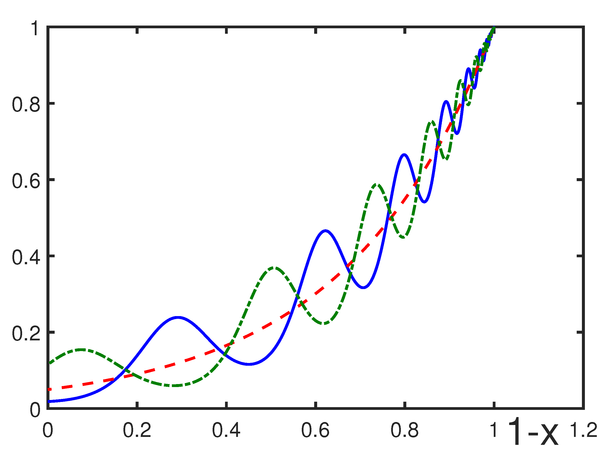
Figure 1. f ( x ) (44) (blue solid line) and f 0 ( x ) (45) (red dashed-dotted line) for α = 1 , a = 3 , b = 1 , φ = 0.1 , with ω = 10 (a) and 50 (b).
Physics 07 00009 g001
Figure 2. f ( x ) for φ = 0.1 (blue solid line) and 10 (green dashed-dotted line), and f 0 ( x ) (red dashed line) for α = 1 , a = 3 , b = 1 , and ω = 10 . Note that f 0 ( x ) does not depend on φ .
Physics 07 00009 g002
Figure 3. f ( x ) (blue line) and f 0 ( x ) (red line) for a = 5 , b = 2 , ω = 10 , and φ = 0.1 , with α = 1 (a) and 3 (b).
Physics 07 00009 g003
Figure 4. f ( x ) (blue solid line) and f 0 ( x ) (red dashed-dotted line) for α = 1 , b = 1 , ω = 25 , and φ = 5 , with a = 3 (a) and 5 (b).
Physics 07 00009 g004
Figure 5. f ( x ) (blue solid line) and f 0 ( x ) (red dashed-dotted line) for α = 1 , a = 3 , ω = 10 , and φ = 1 , with b = 1 (a) and 2 (b).
Physics 07 00009 g005
Figure 6. f ( x ) for a = 3 , b = 2 , α = 1 , ω = 10 , μ = 1.1 , and φ = 0.1 , with N = 1 (a), 5 (b), 25 (c), and 70 (d). Note that function f ( x ) does not change its behavior for N > 70 .
Physics 07 00009 g006
Figure 7. f ( x ) for a = 3 , b = 2 , α = 1 , ω = 10 , μ = 1.1 , and φ = 0.5 , with N = 1 (a), 5 (b), 25 (c), and 70 (d). Note that function f ( x ) does not change its behavior for N > 70 .
Physics 07 00009 g007
Figure 8. f ( x ) for b = 2 , α = 1 , ω = 10 , μ = 1.1 , φ = 0.1 , and a = 1 , with N = 1 (a), 5 (b), 25 (c), and 70 (d). Note that function f ( x ) does not change its behavior for N > 70 .
Physics 07 00009 g008
Figure 9. f ( x ) for a = 3 , b = 2 , ω = 10 , μ = 1.1 , φ = 0.1 , and α = 0.3 , with N = 1 (a), 5 (b), 25 (c), and 70 (d). Note that function f ( x ) does not change its behavior for N > 70 .
Physics 07 00009 g009
Figure 10. f ( x ) for a = 3 , b = 2 , μ = 1.1 , φ = 0.1 , α = 1 , and ω = 25 , with N = 1 (a), 5, (b), 25 (c), and 70 (d). Note that function f ( x ) does not change its behavior for N > 70 .
Physics 07 00009 g010
Figure 11. f ( x ) for a = 3 , b = 2 , ω = 25 , α = 1 , and μ = 1.1 , with N = 1 (a), 5 (b), 25 (c), 70 (d), 100 (e), and 200 (f). The parameters φ n are generated as random numbers from the normal distribution with standard deviation of 0.1 and zero mean.
Physics 07 00009 g011
Figure 12. f ( x ) for a = 3 , b = 2 , ω = 25 , α = 1 , and μ = 1.1 , with N = 1 (a), 5 (b), 25 (c), 70 (d), 100 (e), and 200 (f). The parameters φ n are generated as random numbers from the normal distribution with standard deviation of 1 and zero mean.
Physics 07 00009 g012
Table 1. Prediction for the critical point x c and critical exponent α based on the self-similar summation of the asymptotic expansion at x 0 , where x is defined by the expression (13).
k x c α
20.8871.773
30.9992.124
41.1382.957
51.0922.591
60.9981.831
70.9931.783
80.9941.794
90.9941.790
Disclaimer/Publisher’s Note: The statements, opinions and data contained in all publications are solely those of the individual author(s) and contributor(s) and not of MDPI and/or the editor(s). MDPI and/or the editor(s) disclaim responsibility for any injury to people or property resulting from any ideas, methods, instructions or products referred to in the content.