Chaotic Dynamics and Subharmonic Bifurcation of Charged Dilation-AdS Black Hole in Extended Phase Space Subject to Harmonic Excitation

Abstract

In this paper, the chaotic behavior and subharmonic bifurcation in a dynamical model for charged dilation-AdS black holes are investigated in extended phase space using analytical and numerical methods. An analytical expression for the chaotic critical value at the disturbance amplitude is obtained using the Melnikov method, revealing the monotonicity of the threshold values for chaos with charge and frequency, and the coupling parameters between the expansion field and the Maxwell field are studied. It is shown that chaos can be controlled through the system parameters. Meanwhile, an analytical expression for the critical value of the bifurcation of subharmonic orbits at disturbance amplitudes is acquired using the subharmonic Melnikov method. The relationship between the threshold value and the vibration frequency and the order of the subharmonic orbit is studied. This demonstrates that the system undergoes chaotic motion via infinite odd-order subharmonic bifurcations. Finally, numerical simulations are used to verify the analytical results.

1. Introduction

Black hole dynamics involves the cross-fusion of different branches of physics, such as general relativity, quantum mechanics and thermodynamics. By studying the dynamic behavior of black holes, one can promote the cross-fusion of and mutual verification between these branches of physics and explore the evolution law of the universe further. So, it is crucial to study the nonlinear dynamic characteristics of black hole systems. Some conclusions on the dynamics of black holes have been acquired in recent years.

In 1983, the stability of black holes were analyzed in asymptotic AdS-spacetime after the introduction of cosmological constants and it was found that the black hole has thermodynamic properties [1]. Later, in Ref. [2], it was found that chaos-bound violations in charged Bardeen black holes persist throughout spacetime while diminishing with increasing black hole charge or particle charge/angular momentum. In Ref. [3], it was established the correspondence between the thermodynamics of black holes and van der Waals fluids by treating the cosmological constant as thermodynamic pressure. In Ref. [4], solutions for AdS black holes with interior mixmaster chaos were derived through massive vector field couplings, reproducing BKL dynamics. In Ref. [5], quantum-corrected AdS black holes across cosmological backgrounds were investigated and van der Waals thermodynamics with universe-dependent criticality and universal quantum-enhanced chaos featuring was shown. In Ref. [6], the dynamics of spinning test particles around a Schwarzschild black hole with quintessence (SQBH) were investigated using the Mathisson–Papapetrou–Dixon equations. Reference [7] studied deterministic chaos in van der Waals fluids using the Melnikov method [8] and discussed the temporal chaos from thermal fluctuations in quenched unstable spinodal states and the spatial chaos from pressure-tuned periodic perturbations in infinite tubes.

It is natural to consider the possible chaotic behavior in black hole systems in the Melnikov context. Reference [9] extended the method for studying the thermodynamic evolution of van der Waals fluids to the extended phase space of an RN–AdS black hole. It was shown that homogeneity/heterotopic orbital entanglements would occur in the phase space of RN–AdS black holes. The Melnikov method was used to study the critical conditions for the emergence of thermodynamic chaos. Using the Melnikov method, in Ref. [10] the chaotic behavior of Born–Infeld–AdS black holes was investigated and it was shown the Born–Infeld parameters significantly to affect the critical conditions of thermodynamic chaos. Reference [11] investigated the chaotic and critical behaviors in time and space of charged dilation black holes using the Melnikov method and showed that temporal chaos requires critical perturbation amplitudes to be exceeded, while spatial chaos persists unconditionally. Reference [12] investigated the chaotic behaviors in temporal and spatial perturbations for a slowly rotating Kerr–AdS black hole based on the Melnikov method, finding that time chaos is rather to occur with an increasing angular momentum, while spatial chaos is independent of the perturbation amplitude. In Ref. [13], chaotic timelike geodesics in disk-perturbed black hole systems were analyzed by extending the Melnikov method to 2-DOF Hamiltonian systems, demonstrating the splitting and intersection of asymptotic manifolds. Reference [14] studied the orbital chaos induced by periodic shape oscillations in Schwarzschild spacetime through the Melnikov method, showing how prolate–oblate spheroidal deformations trigger chaotic dynamics in long-term test-body motion. Reference [15] invetsigated charged-flat black holes in Rényi extended phase space using the Melnikov method, showing their van der Waals-like phase behavior and chaotic dynamics under thermal perturbations, which reveals the profound connections between the Rényi parameters and cosmological constant effects, and spatial perturbations universally induce chaos. Reference [16] studied the chaotic dynamics of pulsating extended bodies in spherically symmetric spacetimes (including RN and Ayón–Beato–García black holes) through the Melnikov method, demonstrating that radial oscillations induce homoclinic intersections and consequent chaos in modified gravity scenarios. Reference [17] investigated the chaos in charged Gauss–Bonnet AdS black holes within extended phase space using the Melnikov method, showing that temporal chaos emerges when the thermal quench parameter $\gamma$ surpasses a critical value dependent on the Gauss–Bonnet coupling $\alpha$ and charge Q, while spatial chaos persists universally regardless of charge. Reference [18] studied the chaotic particle motion around Schwarzschild black holes using the Melnikov method, showing that unstable circular orbits generate homoclinic trajectories which become chaotic under periodic metric perturbations. Reference [19] investigated the spin effects of Kerr black holes on the charged particle dynamics in magnetized accretion flows, which showed that the frame-dragging induced chaos in the regularity transitions. Reference [20] analyzed magnetized Schwarzschild chaos and demonstrated that the magnetic curvature induces neutral particle chaos while the electromagnetic forces govern the charged particle dynamics. Global dynamic behaviors also profoundly affect the properties of black holes. Therefore, we investigate here the global dynamics of black holes.

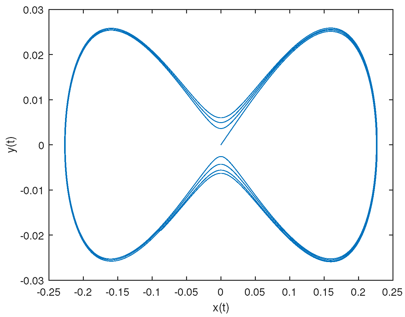
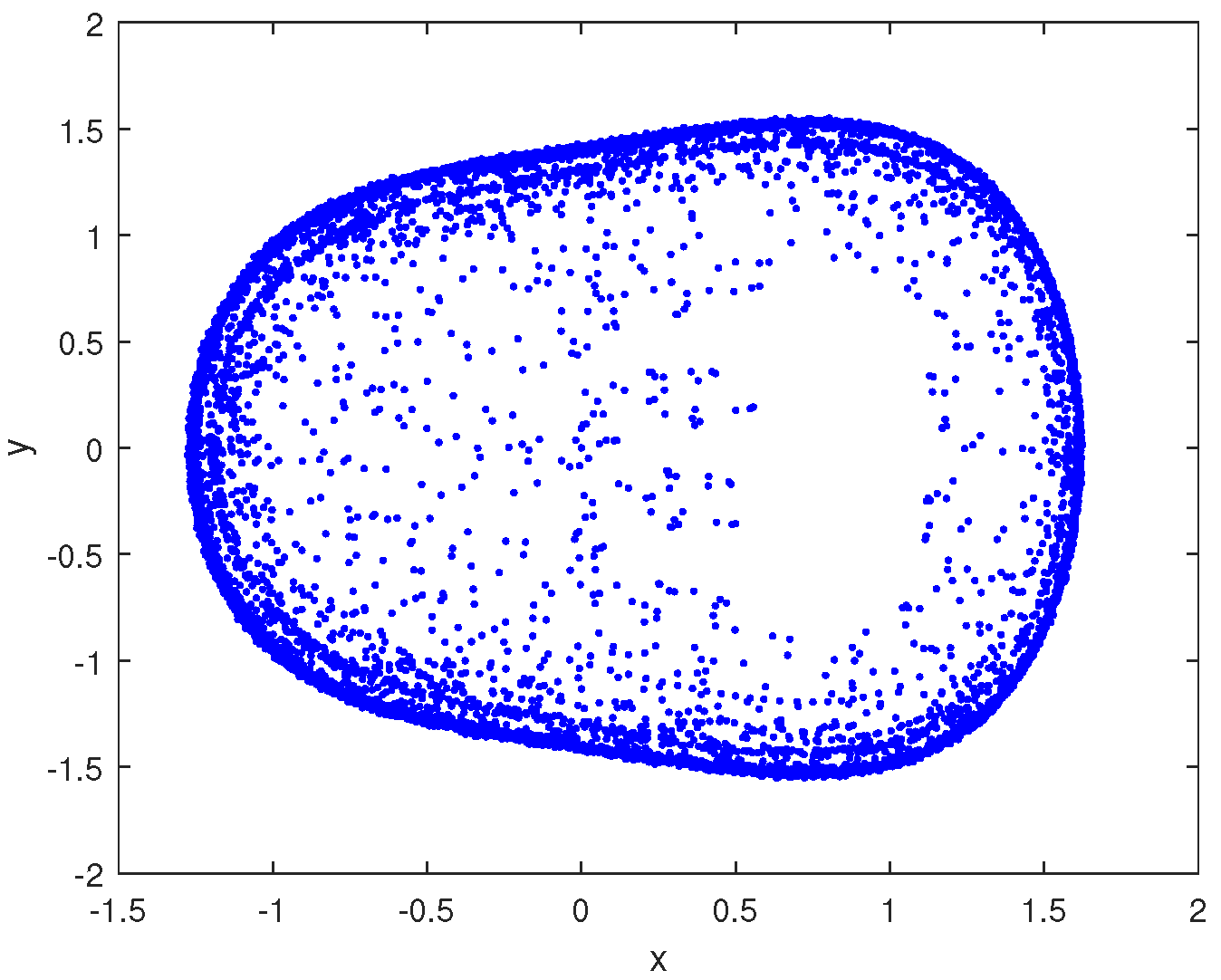
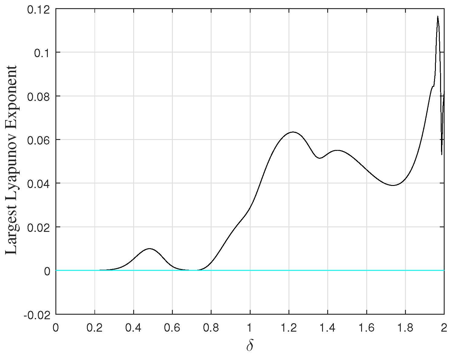
In this paper, the global dynamics, including the chaos and subharmonic bifurcation, in a dynamical model of charged expanding AdS-black holes in extended phase space is investigated using analytical and numerical methods. The monotonicity between the chaos threshold and the vibration frequency, the coupling parameters between the expansion field and the Maxwell field, and the charge of the black hole are given and proven analytically. The evolution process of the system from subharmonic bifurcation to chaos is analyzed. This demonstrates that the system can undergo chaotic motion via infinite subharmonic bifurcations of an odd order.

The paper is organized as follows. The derivation of the dynamical system is given in Section 2. In Section 3, the chaotic dynamics of the system is investigated. Section 4 is devoted to the subharmonic bifurcation of this model. Numerical simulations and conclusions are given in Section 5 and Section 6, respectively.

2. The Dynamic Model and Problem Formulation

According to Ref. [11], the action of Einstein–Maxwell theory with a dilation field can be expressed as

$$\begin{array}{c}\hfill \mathcal{I}={\displaystyle \frac{1}{16\pi }}\int {\mathrm{d}}^{4}X\sqrt{-g}[\mathcal{R}-2{(\nabla \phi )}^2-2\mathsf{\Lambda }{e}^{2\eta \phi }-{\displaystyle \frac{2{\eta }^2}{b^2({\eta }^2-1)}}{e}^{2\phi /\eta }-e^{-2\eta \phi }{F}_{\mu v}{F}^{\mu v}],\end{array}$$

(1)

where $\phi$ is the dilation field, and the electromagnetic tensor $F_{\mu \nu }=\partial {[}_{\mu }{A}_{\nu }]$ is related to the potential vector $A_{\nu }$, X denotes the four-vector, g is the determinant of the metric tensor $g_{\mu \nu }$ with the indexes of Greek letters taking values 0 (time), and 1, 2, and 3 (space) coordinates, $\mathcal{R}$ is the Ricci scalar, $\mathsf{\Lambda }$ is the cosmological constant. $\eta$ is the coupling parameter between the dilation and Maxwell fields, and b is a positive constant. From Equation (1), one obtains a solution for a spherical symmetric black hole and a metric of the form

$$\begin{array}{c}\hfill \mathrm{d}{\widehat{s}}^2=-f\left(r\right)\mathrm{d}{t}^2+{\displaystyle \frac{1}{f\left(r\right)}}\mathrm{d}{r}^2+r^2{\mathrm{R}}^2\left(r\right)(\mathrm{d}{\mathsf{\Theta }}^2+{sin}^2\mathsf{\Theta }\mathrm{d}{\mathsf{\Phi }}^2),\end{array}$$

(2)

where ($r,\mathsf{\Theta },\mathsf{\Phi }$) are the spherical coordinates,

$$\begin{array}{c}\hfill f\left(r\right)=-{\displaystyle \frac{{\eta }^2+1}{{\eta }^2-1}}{\left({\displaystyle \frac{b}{r}}\right)}^{-2\gamma }-{\displaystyle \frac{m}{r^{1-2\gamma }}}-{\displaystyle \frac{3{(\eta +1)}^2{r}^2}{l^2({\eta }^2-3)}}{\left({\displaystyle \frac{b}{r}}\right)}^{2\gamma }+{\displaystyle \frac{q^2({\eta }^2+1)}{r^2}}{\left({\displaystyle \frac{b}{r}}\right)}^{-2\gamma },\end{array}$$

(3)

$$\begin{array}{c}\hfill \phi \left(r\right)={\displaystyle \frac{\eta }{{\eta }^2+1}}ln\left({\displaystyle \frac{b}{r}}\right),\mathrm{R}\left(r\right)={\left({\displaystyle \frac{b}{r}}\right)}^{\gamma },F_{tr}={\displaystyle \frac{e^{2\eta \phi }}{r^2{\mathrm{R}}^2}}.\end{array}$$

(4)

Here, $\gamma ={\displaystyle \frac{{\eta }^2}{{\eta }^2+1}}$, q is the black-hole charge, the parameter m is associated with the ADM mass $\mathcal{M}$ of black hole (2) through $m=2({\eta }^2+1)b^{-2\gamma }\mathcal{M}$, and $F_{tr}$ represents the components of electromagnetic field in the directions of t and r. From Equation (2), the Hawking temperature T and entropy S read:

$$\begin{array}{cc}\hfill T=& -{\displaystyle \frac{({\eta }^2+1)}{4\pi ({\eta }^2-1)r_{+}}}{\left({\displaystyle \frac{b}{r_{+}}}\right)}^{-2\gamma }-{\displaystyle \frac{\mathsf{\Lambda }({\eta }^2+1)r_{+}}{4\pi }}{\left({\displaystyle \frac{b}{r_{+}}}\right)}^{2\gamma }-{\displaystyle \frac{q^2({\eta }^2+1)}{4\pi r_{+}^3}}{\left({\displaystyle \frac{b}{r_{+}}}\right)}^{-2\gamma },\hfill \\ \hfill S=& \pi b^{2\gamma }{r}_{+}^{2(1-\gamma )},\hfill \end{array}$$

(5)

where $r_{+}$ is the event horizon radius. Introducing the thermodynamic pressure P, its conjugate quantity as the volume V and the electric potential U yields

$$\begin{array}{c}\hfill P=-{\displaystyle \frac{(3+{\eta }^2)b^{2\gamma }\mathsf{\Lambda }}{8\pi (3-{\eta }^2)r_{+}^{2\gamma }}},V={\displaystyle \frac{4\pi (1+{\eta }^2)b^{2\gamma }}{3+{\eta }^2}}{r}_{+}^{{\displaystyle \frac{3+{\eta }^2}{1+{\eta }^2}}},U={\displaystyle \frac{q}{r_{+}}}.\end{array}$$

(6)

The first law of thermodynamics and the corresponding Smarr formula in extended phase space are then expressed as

$$\begin{array}{cc}\hfill dM& =Tds+Udq+VdP\hfill \\ \hfill \mathrm{and}M& =2(1-\gamma )TS+Uq+(4\gamma -2)VP,\hfill \end{array}$$

(7)

respectively.

Based on Equations (5) and (6), the thermodynamic pressure P then reads

$$\begin{array}{c}\hfill P(\theta ,T)={\displaystyle \frac{T}{\theta }}+{\displaystyle \frac{b^{-2\gamma }\left[\frac{{(3-{\eta }^2)}^{1-2\gamma }}{2({\eta }^2-1){({\eta }^2+1)}^2{(3+{\eta }^2)}^{1-2\gamma }}+\frac{2q^2{(3+{\eta }^2)}^{2\gamma -3}}{{\theta }^2{(3-\eta )}^{2\gamma -3}}\right]}{2^{2\gamma }\pi {\theta }^{2(1-\gamma ){({\eta }^2+1)}^{2(\gamma -2)}}}},\end{array}$$

(8)

where $\theta$ is the specific volume.

According to Refs. [17,21], one can assume that the flow of the charged dilation-AdS black hole moves along the x-axis of a fixed-volume unit cross-section. Then, using Eulerian coordinates to describe the mass of the column of fluid of the unit cross-section between points x and $x_{*}$ yields

$$\begin{array}{c}\hfill M={\int }_{x_{*}}^x\rho (\xi ,t)\mathrm{d}\xi .\end{array}$$

(9)

Note that M in Equations (7) and (9) is not the same parameter. From the definition of M, one can deduce that x can be phrased as $x(M,t)$, and $y(M,t)=\dot{x}(M,t)$ defines the velocity (where the dot on the top denotes the time-derivative). Then, $x_M(M,t)\equiv {\displaystyle \frac{\partial x(M,t)}{\partial M}}=\rho {[x(M,t),t]}^{-1}$ is defined as the specific volume $\theta (M,t)$. According to these equations and Ref. [21], one can deduce that the flow of the charged dilation-Ads black hole can be described using a dynamical system with a balance equation for the mass and the momentum, i.e.,

$$\begin{array}{c}\hfill {\displaystyle \frac{\partial \theta }{\partial t}}={\displaystyle \frac{\partial y}{\partial M}},\\ \hfill {\displaystyle \frac{\partial y}{\partial t}}={\displaystyle \frac{\partial \tau }{\partial M}},\end{array}$$

(10)

where $\tau$ is the Piola stress. It can be deduced that the black hole system is thermoelastic, isotropic and slightly viscous [11,21]; thus, $\tau$ reads

$$\begin{array}{c}\hfill \tau =-P(\theta ,T)+\mu y_M-A{\theta }_{MM}.\end{array}$$

(11)

Here and in what follows, the variables in the subscript denote the derivatives, such as ${\mathcal{F}}_a=\partial \mathcal{F}/\partial a$, ${\mathcal{F}}_{aa}={\partial }^2\mathcal{F}/\partial a^2$, ${\mathcal{F}}_{aB}={\partial }^2\mathcal{F}/\partial a\partial B$ etc. A is a positive coefficient, and $\mu$ is a relatively small positive constant viscosity. Substituting Equation (10) into Equation (11) and introducing the transformation $\widehat{M}=sM,\widehat{t}=st,\widehat{x}=sx$, and $\mu =ϵ{\mu }_0$, where $ϵ$ is a perturbation parameter and ${\mu }_0$ is the proper viscosity, Equation (11) can be rewritten as follows:

$$\begin{array}{c}\hfill \ddot{x}\left(t\right)=-P{(\theta ,T)}_M+ϵ{\mu }_0{y}_{MM}-A{s}^2{\theta }_{MMM},\end{array}$$

(12)

where $M\in [0,2\pi ]$. Here, the hats are omitted for brevity.

Similar to that in Ref. [11], the values of the positive parameters are fixed, the system pressure P changes with temperature T and specific volume $\theta$, and there exists a critical temperature $T_c$ in the system. Specifically, when $T<T_c$, the system is considered to undergo a black hole phase transition with a change in $\theta$: $[0,{\theta }_1]$ corresponds to a relatively small black hole phase, $[{\theta }_2,\infty ]$ is a large enough black hole phase, and $[{\theta }_1,{\theta }_2]$ corresponds to a region in which such small–large black hole phases coexist. The chaotic phenomena in the system under the coexistence of those large and small black holes is studied in the Sections to follow. According to Ref. [7], taking $T_0<T_c$ and $\theta ={\theta }_0$$\left({\displaystyle \frac{{\partial }^{2}P(\theta ,T)}{{\partial }^2\theta }}=0\right)$$\in [{\theta }_1,{\theta }_2]$, the absolute temperature close to $T_0$ can be expressed as $T=T_0+ϵ\delta \cos \left(\omega t\right)\cos M$ with small time-periodic fluctuations, where $\omega$ is the frequency and $\delta$ is the disturbance amplitude. To perform a perturbation analysis, we expand Equation (8) of $(T_0,{\theta }_0)$ into a Taylor series. Then, we set

$$\begin{array}{cc}\hfill P(\theta ,T)& =P({\theta }_0,T_0)+P_{\theta }({\theta }_0,T_0)(\theta -{\theta }_0)+P_T({\theta }_0,T_0)(T-T_0)\hfill \\ & +P_{\theta T}({\theta }_0,T_0)(\theta -{\theta }_0)(T-T_0)+{\displaystyle \frac{P_{\theta \theta \theta }({\theta }_0,T_0)}{3!}}{(\theta -{\theta }_0)}^3\hfill \\ & +{\displaystyle \frac{P_{\theta \theta T}({\theta }_0,T_0)}{2}}{(\theta -{\theta }_0)}^2(T-T_0)+\dots ,\hfill \end{array}$$

(13)

where $P_{\theta \theta }({\theta }_0,T_0)=0$ and $P_{TT}({\theta }_0,T_0)$, $P_{\theta TT}({\theta }_0,T_0)$, and $P_{TTT}({\theta }_0,T_0)$ equal zero because Equation (8) contains only the first term of T,

$$\begin{array}{cc}\hfill & P_T({\theta }_0,T_0)={\displaystyle \frac{1}{{\theta }_0}},P_{\theta T}({\theta }_0,T_0)=-{\displaystyle \frac{1}{{\theta }_0^2}},P_{\theta \theta T}({\theta }_0,T_0)={\displaystyle \frac{2}{{{\theta }_0}^3}},\hfill \\ & P_{\theta \theta \theta }({\theta }_0,T_0)=-{\displaystyle \frac{6T_0}{{{\theta }_0}^4}}+{\displaystyle \frac{2{\left[\left(3-{\eta }^2\right)\right]}^{\frac{1-{\eta }^2}{1+{\eta }^2}}\left(2+{\eta }^2\right)\left[{\left(3+{\eta }^2\right)}^3{{\theta }_0}^2+2\left({\eta }^2-1\right)\left(2{\eta }^2+5\right)\left(5{\eta }^2+7\right){\left({\eta }^4-2{\eta }^2-3\right)}^2{q}^2\right]}{\pi \left(1-{\eta }^2\right)4^{\frac{{\eta }^2}{1+{\eta }^2}}{b}^{\frac{2{\eta }^2}{1+{\eta }^2}}{\left(1+{\eta }^2\right)}^{\frac{3{\eta }^2+1}{1+{\eta }^2}}{\left(3+{\eta }^2\right)}^{\frac{3+{\eta }^2}{1+{\eta }^2}}{{\theta }_0}^{\frac{35{\eta }^2+7}{1+{\eta }^2}}}},\hfill \\ \hfill & P_{\theta }({\theta }_0,T_0)=-{\displaystyle \frac{T_0}{{{\theta }_0}^2}}+{\displaystyle \frac{{\left[\left(3-{\eta }^2\right)\left(1+{\eta }^2\right)\right]}^{\frac{1-{\eta }^2}{1+{\eta }^2}}\left[4\left({\eta }^4+{\eta }^2-2\right){\left({\eta }^4-2{\eta }^2-3\right)}^2{q}^2+{\left(3+{\eta }^2\right)}^2{{\theta }_0}^2\right]}{\pi \left(1-{\eta }^2\right)4^{\frac{{\eta }^2}{1+{\eta }^2}}{b}^{\frac{2{\eta }^2}{1+{\eta }^2}}{\left({\eta }^2+3\right)}^{\frac{{\eta }^2+3}{1+{\eta }^2}}{\theta }^{\frac{3{\eta }^2+5}{{\eta }^2+1}}}}.\hfill \end{array}$$

(14)

As soon as $M\in [0,2\pi ]$, $\theta (M,t)$ and $y(M,t)$ can be Fourier-expanded in the vicinity of ${\theta }_0$:

$$\begin{array}{cc}\hfill \theta (M,t)& =x_M(M,t)={\theta }_0+x_1\left(t\right)\cos M+x_2\left(t\right)\cos \left(2M\right)+x_3\left(t\right)\cos \left(3M\right)+\dots ,\hfill \\ \hfill y(M,t)& =\dot{x}(M,t)=y_1\left(t\right)\sin M+y_2\left(t\right)\sin \left(2M\right)+y_3\left(t\right)\sin \left(3M\right)+\dots ,\hfill \end{array}$$

(15)

where $x_i$ and $y_i$ are the parameters of the hydrodynamical model which describes the deviation from the initial equilibrium state with $\theta ={\theta }_0$. In this paper, we consider only the first mode ($x_1\left(t\right),y_1\left(t\right)$) and, for brevity, omit the subscript.

With these conditions, Equation (12) reads:

$$\begin{array}{c}\hfill \ddot{x}=(P_{\theta }-A{s}^2)x+ϵ\left(P_T+{\displaystyle \frac{3P_{\theta \theta T}}{8}}{x}^2\right)\delta \cos \omega t+{\displaystyle \frac{P_{\theta \theta \theta }}{8}}{x}^3-ϵ{\mu }_{0}sy,\end{array}$$

(16)

where $P_{\theta }$, $P_T$, $P_{\theta \theta T}$, and $P_{\theta \theta \theta }$ are $P_{\theta }({\theta }_0,T_0)$, $P_T({\theta }_0,T_0)$, $P_{\theta \theta T}({\theta }_0,T_0)$, and $P_{\theta \theta \theta }({\theta }_0,T_0)$, respectively. Since $\dot{x}=y$, Equation (16) can be rewritten in the following form:

$$\left\{\begin{array}{c}\dot{x}=y,\hfill \\ \\ \dot{y}=(P_{\theta }-A{s}^2)x+ϵ\left(P_T+{\displaystyle \frac{3P_{\theta \theta T}}{8}}{x}^2\right)\delta \cos \omega t+{\displaystyle \frac{P_{\theta \theta \theta }}{8}}{x}^3-ϵ{\mu }_{0}sy.\hfill \end{array}\right.$$

(17)

In terms of $z={[x,y]}^T$ and $a^2=(P_{\theta }-A{s}^2)$, Equation (17) reads

$$\begin{array}{cc}\hfill & \dot{z}=\left[\begin{array}{c}y\\ a^{2}x+{\displaystyle \frac{P_{\theta \theta \theta }}{8}}{x}^3\end{array}\right]+ϵ\left[\begin{array}{c}0\\ \left(P_T+{\displaystyle \frac{3P_{\theta \theta T}}{8}}\right)x^2\delta \cos \omega t+{\displaystyle \frac{P_{\theta \theta \theta }}{8}}{x}^3-{\mu }_{0}sy\end{array}\right].\hfill \end{array}$$

(18)

3. Analysis of the Unperturbed System

When $ϵ=0$, the system (17) transforms to

$$\left\{\begin{array}{c}\dot{x}=y,\hfill \\ \\ \dot{y}=a^{2}x+{\displaystyle \frac{P_{\theta \theta \theta }}{8}}{x}^3,\hfill \end{array}\right.$$

(19)

with the Hamiltonian

$$H(x,y)={\displaystyle \frac{y^2}{2}}-{\displaystyle \frac{a^2{x}^2}{2}}-{\displaystyle \frac{P_{\theta \theta \theta }{x}^4}{32}}\equiv h.$$

(20)

Three equilibrium points are identified in the system (19): the saddle $O(0,0)$ and two centers $A_{\pm }=\left(\pm 2a\sqrt{{\displaystyle \frac{2}{-P_{\theta \theta \theta }}}},0\right)$. When $h=0$, Equation (19) has an analytical solution and yields

$$\left[\begin{array}{c}{x}_0\left(t\right)\\ y_0\left(t\right)\end{array}\right]=\left[\begin{array}{c}{\displaystyle \frac{\pm 4a}{\sqrt{(-P_{\theta \theta \theta })}}}\mathrm{sech}\left(at\right)\\ {\displaystyle \frac{\mp 4a^2}{\sqrt{(-P_{\theta \theta \theta })}}}\mathrm{sech}\left(at\right)\tanh \left(at\right)\end{array}\right].$$

(21)

In solution (21), the stable and unstable manifolds of the hyperbolic saddle point O overlap to form a pair of homologous orbits symmetric about the ordinate axis, with positive and negative half-orbits around the center. This is shown in Figure 1.

When $0<h<+\infty$, Equation (20) has a family of periodic solutions around the saddle point O that can be represented by h, which yields

$$\left[\begin{array}{c}x\left(t\right)\\ y\left(t\right)\end{array}\right]=\left[\begin{array}{c}B\mathrm{cn}(\mathsf{\Omega }t,k)\\ -B\mathsf{\Omega }\mathrm{sn}(\mathsf{\Omega }t,k)\mathrm{dn}(\mathsf{\Omega }t,k)\end{array}\right],$$

(22)

where $A^2=4\sqrt{{\displaystyle \frac{4a^4}{{P_{\theta \theta \theta }}^2}}+{\displaystyle \frac{2h}{-P_{\theta \theta \theta }}}}+{\displaystyle \frac{8a^2}{P_{\theta \theta \theta }}}$, $B^2=4\sqrt{{\displaystyle \frac{4a^4}{{P_{\theta \theta \theta }}^2}}-{\displaystyle \frac{2h}{-P_{\theta \theta \theta }}}}+{\displaystyle \frac{8a^2}{P_{\theta \theta \theta }}}$, $\mathsf{\Omega }=\sqrt{A^2+B^2}/{\displaystyle \frac{4}{\sqrt{-P_{\theta \theta \theta }}}}=a/\sqrt{2k^2-1}$, and $k=B/\sqrt{A^2+B^2}$. Thus, B and $\mathsf{\Omega }$ can be represented by k as $B^2={\displaystyle \frac{16a^2{k}^2}{-P_{\theta \theta \theta }(2k^2-1)}}$ and ${\mathsf{\Omega }}^2={\displaystyle \frac{a^2}{2k^2-1}}$, respectively. $\mathcal{T}\left(k\right)={\displaystyle \frac{4K\left(k\right)}{\mathsf{\Omega }}}={\displaystyle \frac{4}{a}}\sqrt{2k^2-1}K\left(k\right)$ is the period of the orbit (22), where $K\left(k\right)$ is the Legendre complete elliptic integral of the first kind.

4. Chaotic Motion in the System

The chaotic phenomena in dynamic systems can be studied analytically using the Melnikov method. The method is commonly used in various areas, such as for an extended Duffing–van der Pol oscillator with a nonlinear quintic term [22], a symmetric gyro-subjected system [23], the oscillatory nonlinear dynamic system of a turbine rotor [24], a conveyor belt system featuring bilateral rigid restraints interconnected via inclined springs and dampening elements [25], a cantilever beam that is supported by obliquely positioned springs and subjected to bilateral asymmetric rigid constraints [26], a Rayleigh–Duffing oscillator subjected to both non-smooth periodic perturbations and harmonic excitation [27], spherical shells with incompressible hyperelastic properties [28], a bistable piezoelectric energy harvester [29] etc. As so, also in this paper, the chaotic motion of the system (17) is studied using the Melnikov method.

4.1. Melnikov Analysis and Thresholds for Chaotic Systems

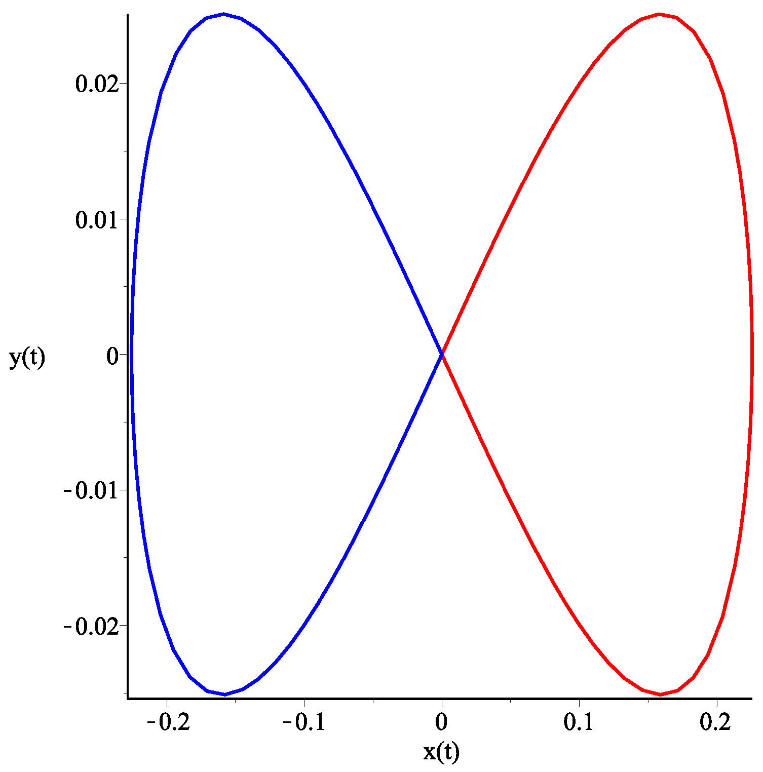
Calculating the Melnikov function for the given system (17) along the homoclinic paths

$$\begin{array}{ccc}M\left(t_0\right)\hfill & =\hfill & {\int }_{-\infty }^{\infty }{y}_0\left(t\right)\left[\left(P_T+{\displaystyle \frac{3P_{\theta \theta T}}{8}}{x}_0^2\left(t\right)\right)\delta \cos \omega t-{\mu }_{0}s{y}_0\left(t\right)\right]\mathrm{d}t\hfill \\ \\ \hfill & =\hfill & {\int }_{-\infty }^{\infty }{\displaystyle \frac{\mp 4a^2}{{(-P_{\theta \theta \theta })}^{\frac{1}{2}}}}\mathrm{sech}\left(at\right)\tanh \left(at\right)\left[\left(P_T+{\displaystyle \frac{3P_{\theta \theta T}}{8}}{\displaystyle \frac{4a}{{(-P_{\theta \theta \theta })}^{\frac{1}{2}}}}{\mathrm{sech}}^2\left(at\right)\right)\right.\delta \cos \omega (t+t_0)\hfill \\ \\ \hfill & \hfill & -{\mu }_{0}su]{\displaystyle \frac{\mp 4a^2}{{(-P_{\theta \theta \theta })}^{\frac{1}{2}}}}\mathrm{sech}\left(at\right)\tanh \left(at\right)\mathrm{d}t\hfill \\ \\ \hfill & \equiv \hfill & P_T\delta I_1+{\displaystyle \frac{3P_{\theta \theta T}}{8}}\delta I_2-{\mu }_{0}s{I}_3,\hfill \end{array}$$

(23)

for which, using the residue theorem and function transformation, one obtains the integrals

$$\begin{array}{ccc}{I}_1\hfill & =\hfill & {\int }_{-\infty }^{+\infty }{y}_0\left(t\right)\cos \omega (t-t_0)\mathrm{d}t=\mp {\displaystyle \frac{4\pi \omega }{{(-P_{\theta \theta \theta })}^{\frac{1}{2}}}}\sin \left(\omega t_0\right)\mathrm{sech}{\displaystyle \frac{\pi \omega }{2a}},\hfill \\ \\ I_2\hfill & =\hfill & {\int }_{-\infty }^{+\infty }{y}_0\left(t\right)x_0^2\left(t\right)\cos \omega (t-t_0)\mathrm{d}t=\mp {\displaystyle \frac{32\pi (a^2+{\omega }^2)\omega }{{(-3P_{\theta \theta \theta })}^{\frac{3}{2}}\cosh \frac{\omega \pi }{2a}}}\sin \left(\omega t_0\right),\hfill \\ \\ I_3\hfill & =\hfill & {\int }_{-\infty }^{+\infty }{y}_0^2\left(t\right)\mathrm{d}t={\displaystyle \frac{32a^3}{-3P_{\theta \theta \theta }}}.\hfill \end{array}$$

(24)

Thus, $\mathit{M}\left(t_0\right)$ has simple zeros if

$${\displaystyle \frac{{\mu }_{0}s}{\delta \omega }}\le {\displaystyle \frac{-3P_{\theta \theta \theta }}{8a^3}}\mathrm{sech}\left({\displaystyle \frac{\pi \omega }{2a}}\right)\left[{\displaystyle \frac{P_T\pi }{{(-P_{\theta \theta \theta })}^{\frac{1}{2}}}}+{\displaystyle \frac{P_{\theta \theta T}\pi (a^2+{\omega }^2)}{{(-P_{\theta \theta \theta })}^{\frac{3}{2}}}}\right].$$

(25)

4.2. The Chaotic Threshold of the System

Now, let us analyze this system’s chaotic threshold value with certain parameters based on Ref. [11], fixing the system’s constant coefficients to $b=1,A=0.2,s=0.001$, taking the proper viscosity ${\mu }_0=0.1$, and setting the perturbation $ϵ=0.01$. Equation (25) can be rewritten as follows:

$$\delta \ge {\displaystyle \frac{{\mu }_{0}s}{\omega \frac{-3P_{\theta \theta \theta }}{8a^3}\mathrm{sech}\left(\frac{\pi \omega }{2a}\right)\left[\frac{P_T\pi }{{(-P_{\theta \theta \theta })}^{\frac{1}{2}}}+\frac{P_{\theta \theta T}\pi (a^2+{\omega }^2)}{{(-P_{\theta \theta \theta })}^{\frac{3}{2}}}\right]}}\equiv R.$$

(26)

R is the chaotic threshold which is related only to $\eta$, q (via $P_{\theta \theta \theta }$), and $\omega$. The influence of the other parameters on R is discussed by fixing the values of two to achieve the purpose of controlling the chaos threshold, and the following three cases are discussed as follows. Taking q close to 1, the system represents an ideal black hole whose physical properties can be fully determined using the aforementioned parameters. Taking $\eta$ as a small enough valuethe influence of the dilation field on the electromagnetic field becomes relatively weak, and the electromagnetic radiation of the black hole follows rather standard thermodynamic laws. We choose quite a small value for $\omega$ to ensure the periodicity of the perturbations. All the parameters are set to the values given just above.

4.2.1. Case 1: Fixed $\eta$ and q

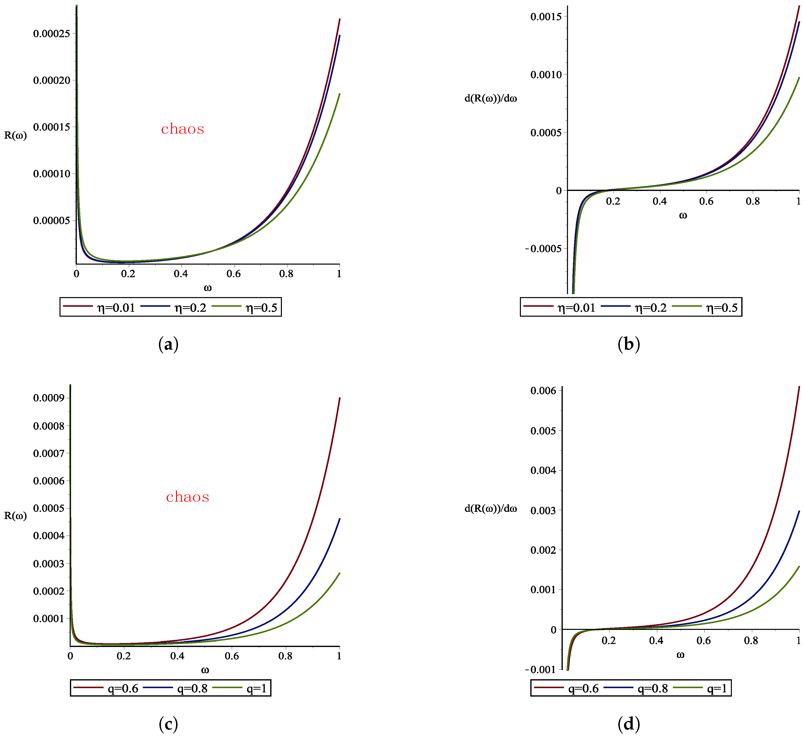
Figure 2 shows the curve of the chaotic threshold $R\left(\omega \right)$ (26) and the change in the chaotic threshold rate ${\displaystyle \frac{\mathrm{d}R\left(\omega \right)}{\mathrm{d}\omega }}$ with the frequency $\omega$ using the parameters defined just above for different values of $\eta$ and q. One can see that the shape of and trend in the curve are nearly the same, what indicates that proper adjustment of the values of $\eta$ and q do not change the direction of the chaotic threshold $R\left(\omega \right)$. Therefore, it is reasonable and complete to discuss the characteristics of the chaotic threshold when $q=1$ and $\eta =0.01$. (Specifically, $T_0=0.0315<T_c$ and ${\theta }_0=4.173$ can be determined based on these values).

Conclusion 1.

For $q=1$ and $\eta =0.01$, the chaotic threshold decreases monotonically as $\omega$ increases for $\omega \in$ $[0,0.170]$ and, conversely, the threshold increases monotonically with $\omega$ for $\omega \in$ $[0.170,+\infty ]$.

4.2.2. Case 2: Fixed $\omega$ and q

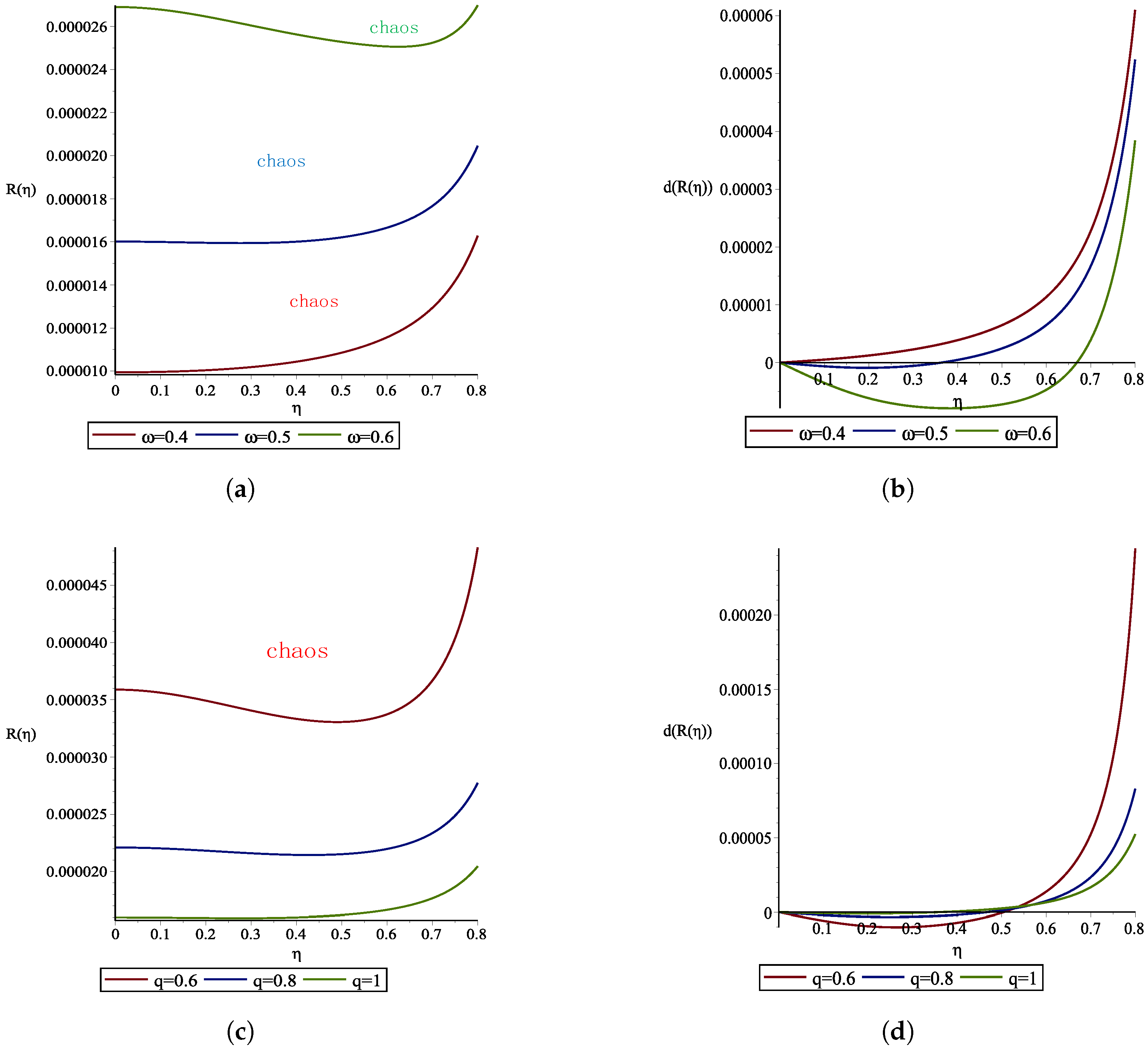
Figure 3 shows the curve in the chaotic threshold $R\left(\eta \right)$ (26) and the change in the chaotic threshold rate ${\displaystyle \frac{\mathrm{d}R\left(\eta \right)}{\mathrm{d}\eta }}$ as a function of $\eta$ for different values for $\omega$ and q using the above-defined parameters. As due to Conclusion 1 of Section 4.2.1, the change in the values of q and $\omega$ has little effect on the trend in the chaotic threshold $R\left(\eta \right)$. Therefore, it is reasonable and complete to discuss the characteristics of the chaotic threshold when $\omega =0.5$ and $q=1$.

Conclusion 2.

For $q=1$ and $\omega =0.5$, the chaotic threshold decreases monotonically as $\eta$ increases for $\eta \in$ $[0,0.356]$ and, conversely, the threshold increases monotonically with $\eta$ for $\eta \in$ $[0.356,1)$.

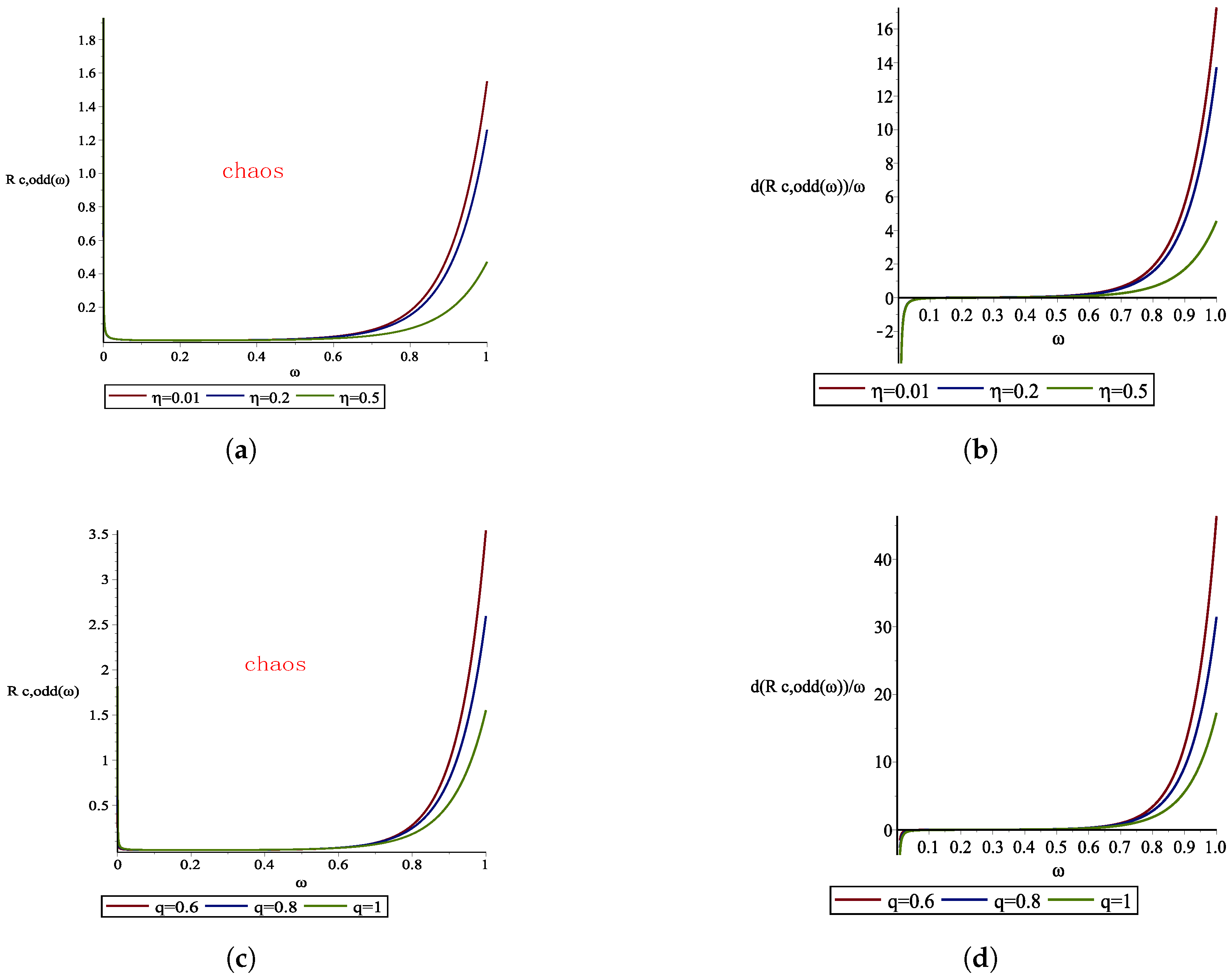
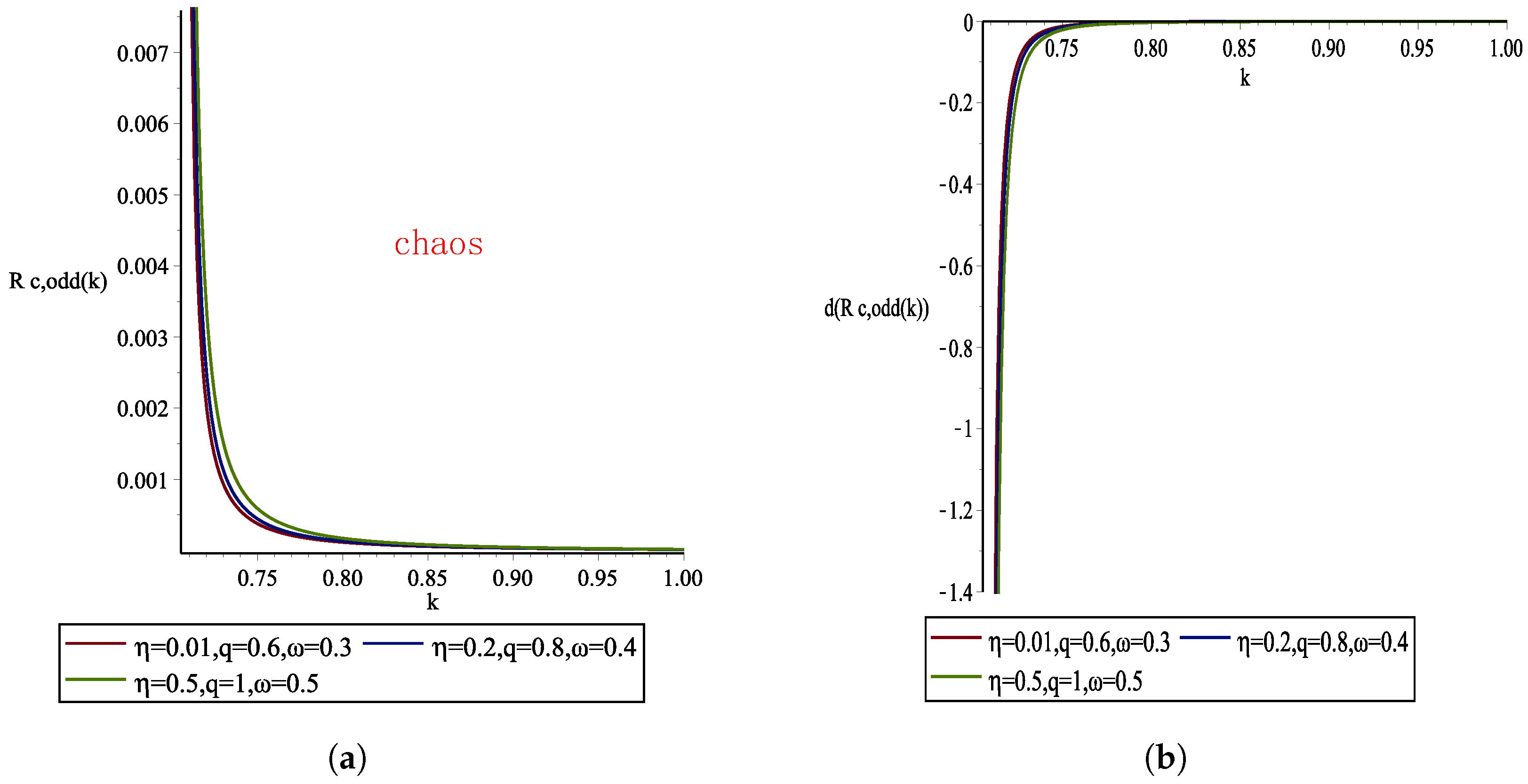
4.2.3. Case 3: Fixed $\omega$ and $\eta$

The curve of the chaotic threshold $R\left(q\right)$ and the change in the chaotic threshold rate ${\displaystyle \frac{\mathrm{d}R\left(q\right)}{\mathrm{d}q}}$ with q for different values of $\omega$ and $\eta$ using the parameters defined above are shown in Figure 4. As due to Conclusion 1 of Section 4.2.1, the change in the values of q and $\omega$ has little effect on the trend in the chaotic threshold $R\left(\eta \right)$. Therefore, it is reasonable and complete to discuss the characteristics of the chaotic threshold when $\omega =0.5,\eta =0.01$.

Conclusion 3.

For $\omega =0.5$ and $\eta =0.01$, the chaotic threshold increases monotonically as q increases for $q\in$ $[0.413,0.415]$ and, conversely, the threshold decreases monotonically with increasing $eta$ for $q\in$ $[0.415,+\infty )$.

5. Subharmonic Bifurcations

In this Section, subharmonic Melnikov method is used to investigate the subharmonic bifurcations of the system (17).

5.1. Parameter Conditions for Subharmonic Bifurcations

For any coprime positive integers m and n, the period of system (17) can be represented by k as $\mathcal{T}\left(k\right)={\displaystyle \frac{4}{a}}\sqrt{2k^2-1}={\displaystyle \frac{m}{n}}\mathcal{T}={\displaystyle \frac{2\pi m}{n\omega }}$, where k is a certain number belonging to $(0,1)$. According to the definition of k and the relationship between k and h (see Equation (22)), one can deduce that $k\in \left({\displaystyle \frac{\sqrt{2}}{2}},1\right)$. Then, calculating the subharmonic Melnikov function to discuss the parametric critical conditions of subharmonic bifurcation yields

$$\begin{array}{cc}{M}^{{\displaystyle \frac{m}{n}}}\left(t_0\right)\hfill & ={\int }_{-{\displaystyle \frac{\mathcal{T}\left(k\right)}{2}}}^{{\displaystyle \frac{\mathcal{T}\left(k\right)}{2}}}y\left(t\right)\left[\left(P_T+{\displaystyle \frac{3P_{\theta \theta T}}{8}}{x}^3\left(t\right)\right)\delta \cos \omega (t+t_0)-{\mu }_{0}sy\left(t\right)\right]\mathrm{d}t\hfill \\ \\ \hfill & =-{\mu }_{0}s{\int }_{-{\displaystyle \frac{\mathcal{T}\left(k\right)}{2}}}^{{\displaystyle \frac{\mathcal{T}\left(k\right)}{2}}}{y}^2\left(t\right)\mathrm{d}t+\delta P_T{\int }_{-{\displaystyle \frac{\mathcal{T}\left(k\right)}{2}}}^{{\displaystyle \frac{\mathcal{T}\left(k\right)}{2}}}y\left(t\right)\cos \omega (t+t_0)\mathrm{d}t\hfill \\ \\ \hfill & +{\displaystyle \frac{3\delta P_{\theta \theta T}}{8}}{\int }_{-{\displaystyle \frac{\mathcal{T}\left(k\right)}{2}}}^{{\displaystyle \frac{\mathcal{T}\left(k\right)}{2}}}{x}^2\left(t\right)y\left(t\right)\cos \omega (t+t_0)\mathrm{d}t\hfill \\ \\ \hfill & \equiv -{\mu }_{0}s{J}_1(m,n)+\delta P_T{J}_2(m,n)+{\displaystyle \frac{3\delta P_{\theta \theta T}}{8}}{J}_3(m,n).\hfill \end{array}$$

(27)

Using the residue theorem and the elliptic function transformation, one obtains

$$\begin{array}{cc}\hfill & J_1(m,n)={\int }_{-{\displaystyle \frac{\mathcal{T}\left(k\right)}{2}}}^{{\displaystyle \frac{\mathcal{T}\left(k\right)}{2}}}{y}^2\left(t\right)\mathrm{d}t={\displaystyle \frac{4B^2\mathsf{\Omega }}{3k^2}}\left[(1-k^2)K\left(k\right)-(1-2k^2)E\left(k\right)\right],\hfill \\ \hfill & J_2(m,n)=\left\{\begin{array}{cc}0\mathrm{when}\hfill & n\ne 1\mathrm{or}m\mathrm{is}\mathrm{even},\hfill \\ \omega sin\left(\omega t_0\right){\displaystyle \frac{2\pi B}{\mathsf{\Omega }k}}\mathrm{sech}\left({\displaystyle \frac{m\pi K^{\prime }\left(k\right)}{2K\left(k\right)}}\right),\hfill & n=1\mathrm{and}m\mathrm{is}\mathrm{odd}\hfill \end{array}\right.\hfill \\ \hfill & J_3(m,n)=\left\{\begin{array}{cc}0\mathrm{when}\hfill & n\ne 1\mathrm{or}m\mathrm{is}\mathrm{even},\hfill \\ {\displaystyle \frac{\omega }{3}}sin\left(\omega t_0\right)\left[{\displaystyle \frac{B^3{m}^2{\pi }^3}{4\mathsf{\Omega }{k}^{2}K{\left(k\right)}^2}}-{\displaystyle \frac{4B^3\pi K{\left(k\right)}^2(1-2k^2)}{4\mathsf{\Omega }{k}^{2}K{\left(k\right)}^2}}\right]\mathrm{sech}\left({\displaystyle \frac{m\pi K^{\prime }\left(k\right)}{2K\left(k\right)}}\right),\hfill & n=1\mathrm{and}m\mathrm{is}\mathrm{odd}\hfill \end{array}\right.\hfill \end{array}$$

(28)

where $E\left(k\right)$ denotes the complete elliptic integral of the second kind and the prime denotes the k-derivative.

Consequently, when

$$\begin{array}{c}\hfill {\displaystyle \frac{{\mu }_{0}s}{\delta }}\le {\displaystyle \frac{P_T{J}_2(m,n)+\frac{3P_{\theta \theta T}}{8}{J}_3(m,n)}{J_1(m,n)}}\end{array}$$

(29)

the system (17) is shown to potentially exhibit chaotic behavior via infinite subharmonic bifurcations of an odd order.

5.2. The Evolution from Subharmonic Bifurcations to Chaos

5.2.1. Case 1: Fixed $\eta$ and q and $k\to 1$

The condition (29) can be expressed as follows:

$$\begin{array}{cc}\hfill \delta & \ge {\displaystyle \frac{{\mu }_{0}s{J}_1(m,n)}{P_T{J}_2(m,n)+\frac{3P_{\theta \theta T}}{8}{J}_3(m,n)}}\equiv R_{c,\mathrm{odd}}^{\infty }\left(\omega \right).\hfill \end{array}$$

(30)

When $\omega >0$ is fixed and $m\to \infty$, one deduces that $k\to 1$ and

$$E\left(k\right)\to 1,K^{\prime }\left(k\right)\to {\displaystyle \frac{\pi }{2}},{\displaystyle \frac{m}{K\left(k\right)}}\to {\displaystyle \frac{2\omega }{a\pi }},$$

and, then,

$$R_{c,\mathrm{odd}}^{\infty }\left(\omega \right)={\displaystyle \frac{8a^2{\mu }_{0}s}{3\pi \omega \sqrt{-P_{\theta \theta \theta }}\left(P_T+\frac{P_{\theta \theta T}({\omega }^2+a^2)}{-P_{\theta \theta \theta }}\right)\mathrm{sech}\left(\frac{\pi \omega }{2a}\right)}}.$$

(31)

The chaotic threshold $R_{c,\mathrm{odd}}^{\infty }\left(\omega \right)$ (31) and the change in the chaotic threshold rate ${\displaystyle \frac{\mathrm{d}{R}_{c,\mathrm{odd}}^{\infty }\left(\omega \right)}{\mathrm{d}\omega }}$ with the frequency $\omega$ for different values of $\eta$ and q using the parameters defined in Section 4.2 are shown in Figure 5. One can see that the shape of and the trend in the chaotic threshold are nearly the same, what indicates that a proper adjustment of the values of $\eta$ and q do change the trend in the chaotic threshold $R\left(\omega \right)$. Therefore, it is reasonable and complete to discuss the characteristics of the chaotic threshold when $q=1$ and $\eta =0.01$. The other two cases (when $\eta$ is fixed or q is fixed) are similar to the Cases 2 and 3 therefore, not discussed here.

With the parameters defined in Section 4.2, one comes to

Conclusion 4.

When $\delta >R_{c,\mathrm{odd}}^{\infty }\left(\omega \right)$, the system is shown to potentially exhibit chaotic behavior via infinite subharmonic bifurcations of an odd order. For $\eta =0.01$ and $q=1$), $R_{c,\mathrm{odd}}^{\infty }\left(\omega \right)$ decreases monotonically as $\omega$ increases for $\omega \in [0,0.170]$, and conversely, $R_{c,\mathrm{odd}}^{\infty }\left(\omega \right)$ increases monotonically with increasing $\omega$ for $\omega \in [0.170,+\infty ]$.

5.2.2. Case 2: Fixed $\eta ,\omega$ and q and $k\in \left({\displaystyle \frac{\sqrt{2}}{2}},1\right)$

The condition (29) can be written as

$$\begin{array}{cc}\hfill \delta & \ge {\displaystyle \frac{{\mu }_{0}s{J}_1(m,n)}{P_T{J}_2(m,n)+\frac{3P_{\theta \theta T}}{8}{J}_3(m,n)}}\hfill \\ \\ & ={\displaystyle \frac{\frac{16a^{3}k}{{(2k^2-1)}^{\frac{3}{2}}\sqrt{-P_{\theta \theta \theta }}}[(1-k^2)K\left(k\right)-(1-2k^2)E\left(k\right)]}{12P_T\pi k\mathrm{sech}\left(\frac{\omega K^{\prime }\left(k\right)}{a}\right)+\frac{3P_{\theta \theta T}}{32}\frac{16a^2{k}^3}{(2k^2-1)\sqrt{-P_{\theta \theta \theta }}}\left[\frac{\pi {\omega }^2}{k{a}^2}-(1-2k^2)\right]\mathrm{sech}\left(\frac{\omega K^{\prime }\left(k\right)}{a}\right)}}\hfill \\ \\ & \equiv R_{c,\mathrm{odd}}^{\infty }\left(k\right).\hfill \end{array}$$

(32)

The chaos critical curve $R_{c,\mathrm{odd}}^{\infty }\left(k\right)$ (32) and the change in its rate ${\displaystyle \frac{\mathrm{d}{R}_{c,\mathrm{odd}}^{\infty }\left(k\right)}{\mathrm{d}k}}$ with k using the parameters defined in Section 4.2 in Figure 6. As due to Conclusion 4, the change in the values of $\eta$, q, and $\omega$ has little effect on the trend in the chaotic threshold $R_{c,\mathrm{odd}}^{\infty }\left(k\right)$. Therefore, it is reasonable and complete to discuss the characteristics of the chaotic threshold when $\eta =0.01$, $q=1$, and $\omega =0.5$.

One concludes:

Conclusion 5.1.

The chatic threshold value of $R_{c,\mathrm{odd}}^{\infty }\left(k\right)$ (32) decreases monotonously with an increase of k for $k\in$ $({\displaystyle \frac{\sqrt{2}}{2}},1)$. Specifically, as $k\to 1$, $R_{c,\mathrm{odd}}^{\infty }\left(k\right)\to 0$, and as $k\to {\displaystyle \frac{\sqrt{2}}{2}}$, $R_{c,\mathrm{odd}}^{\infty }\left(k\right)\to \infty$.

Based on the definition $\mathcal{T}\left(k\right)={\displaystyle \frac{4}{a}}\sqrt{2k^2-1}K\left(k\right)={\displaystyle \frac{2\pi m}{\omega n}}$, one infers that k increases monotonically with m when $m\to \infty$ and $k\to 1$. Then, Conclusion 5.1 can be rewritten:

Conclusion 5.2.

The chaotic threshold $R_{c,\mathrm{odd}}^{\infty }\left(k\right)$ (32) decreases monotonically with an increase of m. Specifically, when m is large enough, $k\to 1$ and $R_{c,\mathrm{odd}}^{\infty }\left(k\right)\to 0$ monotonically.

Meanwhile, considering the ratio of the chaos threshold to the subharmonic bifurcation threshold when $k\to 1$,

$${\displaystyle \frac{R}{R_{c,\mathrm{odd}}^{\infty }}}={\displaystyle \frac{\frac{{\mu }_{0}s}{\frac{-3P_{\theta \theta \theta }}{8a^3}\omega \mathrm{sech}\left(\frac{\pi \omega }{2a}\right)\left[\frac{P_T\pi }{{\left(-P_{\theta \theta \theta }\right)}^{\frac{1}{2}}}+\frac{P_{\theta \theta T}\pi (a^2+{\omega }^2)}{({-P_{\theta \theta \theta })}^{\frac{3}{2}}}\right]}}{\frac{8a^2{\mu }_{0}s}{3\pi \omega \sqrt{-P_{\theta \theta \theta }}\left(P_T+\frac{{\omega }^2+a^2}{-P_{\theta \theta \theta }}\right)\mathrm{sech}\left(\frac{\pi \omega }{2a}\right)}}}=1$$

(33)

for any $\omega$. Synthesizing Conclusion 5.2 and Equation (33), one infers that the system (17) is shown to potentially exhibit chaotic behavior via infinite odd-order subharmonic bifurcations.

6. Numerical Simulations

Now, let us choose the parameters as follows: $A=0.2,s=0.001,b=1,{\mu }_0=0.1,ϵ=0.01,T_0=0.0315,{\theta }_0=4.173,\eta =0.01,q=1,\omega =0.5,{\delta }_1=0.0001<R_{c,\mathrm{odd}}^{\infty }\left(\omega \right)$, and ${\delta }_2=50>R_{c,\mathrm{odd}}^{\infty }\left(\omega \right)$. Using a numerical integration method to simulate the features of the system (17), we find the time history curve, the phase portrait, and the Poincaré section are shown in Figure 7, Figure 8, Figure 9 and Figure 10.

Figure 11 demonstrates that the maximum Lyapunov exponent of system (17) transitions to positive values as the excitation amplitude $\delta$ increases, which confirms the onset of chaotic dynamics. A bifurcation diagram of the excitation amplitude $\delta \in (0,0.5)$ is shown in Figure 12. It can be seen that the system has period-doubling bifurcations and tends towards chaotic motion, what demonstrates that the system exhibits chaotic behavior via infinite subharmonic bifurcations with an increase in the amplitude $\delta$. As one can find that Figure 7, Figure 8, Figure 9, Figure 10, Figure 11 and Figure 12 are all consistent with the theoretical results obtained above.

7. Conclusions

The chaotic behavior and subharmonic bifurcation of dynamical models of charged dilation-AdS black holes in extended phase space have been investigated using analytical and numerical methods. An analytical expression for the chaotic critical threshold dependence on the disturbance amplitude is obtained using the Melnikov method, revealing the monotonicity of the chaotic threshold R with frequency $\omega$, charge q and the coupling parameter $\eta$ between the expansion field and the Maxwell field. This shows that the critical R decreases first and then increases with $\omega$ and q but increases first and then decreases with $\eta$. Meantime, an analytical expression for the threshold of the bifurcation of subharmonic orbits at disturbance amplitudes is obtained using the subharmonic Melnikov method, showing the relationship between frequency $\omega$, the order of the subharmonic orbit m, and the threshold $R_{c,\mathrm{odd}}^{\infty }$. This demonstrates that the system is shown to potentially exhibit chaotic behavior via infinite subharmonic bifurcations of an odd order. The numerical simulation verifies the analytical results.