Non-Stationary Flow of a Viscous Incompressible Electrically Conductive Liquid on a Rotating Plate in the Presence of Media Injection (Suction), Considering Induction and Diffusion Effects

Abstract

The branch of physics known as magnetohydrodynamics (MHD) emerged in the middle of the 20th century. MHD models, being substantially nonlinear, are quite challenging for theoretical study and allow nontrivial consideration only in particular limited cases. Thus, due to the exceptional growth of calculation power, research on MHD is now primarily concentrated on numerical modeling. The achievements are considerable; however, there is a possibility of overlooking some phenomena or missing an optimal approach to modeling and calculating that could be identified with theoretical guidance. The paper presents a theoretical study of a particular class of boundary and initial conditions. The flow of a viscous, electrically conductive fluid on a rotating plate in the presence of a magnetic field is considered. The fluid and the bounding plate rotate together with a constant angular velocity around an axis that is not perpendicular to the plane. The flow is induced by sudden longitudinal vibrations of the plate, injection (suction) of the medium through the plate, and an applied magnetic field directed normal to the plate. The full equation of magnetic induction is used, taking into account both the induction effect and energy dissipation due to the flow of electric currents. An analytical solution of three-dimensional magnetohydrodynamics equations in a half-space bounded by a plate is presented. The solution is given in the form of a superposition of plane waves propagating with certain wave numbers along the y-coordinate axis. For certain regions of system parameters, the vibration of the bounding plate does not cause waves in the media.

1. Introduction

One can trace magnetohydrodynamics (MHD) as a specific theory, where the movements of media and electromagnetic fields are substantially intertwined, back to the paper by Hannes Alfvén [1]. Since then, numerous physical phenomena have been analyzed, modeled, and predicted with the help of this theory. The nature of MHD manifests itself in seemingly heterogeneous processes such as the flow of water in the world’s oceans, the movements of Earth’s liquid core, the dynamics of solar and stellar magnetospheres, and galactic electromagnetic fields.

By its nature, MHD incorporates fluid mechanics as both its part and a special case. A distinctive feature of fluid mechanics is that its foundational equations—the Euler equations for an inviscid fluid and the Navier–Stokes equations for the viscous case—are essentially nonlinear. In contrast, classical electrodynamics was initially created as a linear science; nonlinear terms were added to Maxwell’s equations later, as the complexity of the phenomena under consideration increased. The same is true for quantum mechanics, elasticity theory, and acoustics, which were predominantly developed as linear sciences. In both fluid mechanics and MHD, nontrivial linear motions generally do not exist for most cases of interest. Due to this, since the end of the 20th century, numerical approaches have been developed most intensively.

A large number of investigations are devoted to numerical studies of problems. Here, we outline the solutions related to the specific case in question. References [2,3,4,5] present numerical studies of the problem involving the flow of a gas near a plate with a surface moving against the flow. Additionally, in the boundary layer approximation, a submerged, unswirled jet of viscous, incompressible fluid flowing out of an orifice is considered. Time-periodic and post-transient solutions to this problem are discussed. In Ref. [6], the theory of electromagnetic hydrodynamics is discussed. This theory comprehensively incorporates the electro-ionic structure of the plasma within the hydrodynamic approximation, including the inertia of electrons and ions and their interactions. In Ref. [7], a mathematical model based on a system of differential equations of inhomogeneous multi-component fluid mechanics was proposed. The method allows one to analyze in a single formulation the dynamics and fine structure of flow around obstacles throughout a wide range of flow parameters. Reference [8] provided an analysis of energy transfer mechanisms, including fast direct atomic–molecular and mechanical processes with flow or wave-like propagation with group velocity, as well as slow diffusion. Various types of instabilities in the mechanics of liquids and gases were discussed. In Ref. [9], a swirling flow with a free surface was studied, focusing on a funnel that appears on it, using mathematical modeling. Using video recording methods, in Ref. [10], the evolution of the distribution pattern of the substance of an ink drop freely falling on an agitated liquid surface was traced. Using methods from the theory of singular perturbations in linear and weakly nonlinear approximations, in Ref. [11], the problem of generating beams of periodic internal waves in a viscous was considered, exponentially stratified fluid by a strip oscillating along an inclined plane. Reference [12] focused on hydrodynamics and heat transfer during the downward flow of liquid metal in a rectangular channel with an aspect ratio of approximately 3/1, situated in a coplanar magnetic field. These studies specifically focused on conditions where the channel was non-uniformly (unilaterally) heated.

In MHD, the nature of the interaction between a conducting fluid and a magnetic field is determined by the magnetic Reynolds number ${\mathrm{Re}}_{\mathrm{m}}$. This number is defined as the ratio of inertial forces to the forces that ensure the diffusion of the magnetic field in the conducting fluid: ${\mathrm{Re}}_{\mathrm{m}}=vl/\eta$, where v denotes the typical velocity of the flow, l denotes the typical length scale of the flow, and $\eta$ denotes the magnetic diffusivity. Based on the value of the magnetic Reynolds number, processes in magnetohydrodynamics are divided into three classes [13]. These classes include processes with low (${\mathrm{Re}}_{\mathrm{m}}\ll 1$), moderate (${\mathrm{Re}}_{\mathrm{m}}\sim 1$), and large (${\mathrm{Re}}_{\mathrm{m}}\gg 1$) conductivity. The case of low conductivity occurs in laboratory setups with liquid metals and low-temperature plasma. There, the magnetic field changes little and can be considered to be set from the outside. A conducting liquid moving in this field induces an electric current, which creates the Lorentz force affecting the movement of the liquid and causing the MHD effects. In the opposite scenario, that is, in cases of high conductivity of the medium or its large dimensions (conditions met by astrophysical objects and the hot plasma of thermonuclear devices), the diffusion of the magnetic field can be neglected. This is the case with hydrodynamic approximation, when transport dominates over diffusion. In the general case, changes in the magnetic field result from its transport by a moving conducting substance and diffusion relative to this substance. When considering both processes, it is necessary to use the complete induction equation.

The current study is based on the earlier results [14,15,16,17,18,19]. In Ref. [14], the non-stationary motion of a viscous fluid bounded by a moving flat plate in the absence of a magnetic field was studied. In Ref. [15], a post-transient flow of a viscous incompressible fluid on a rotating plate was considered in the absence of medium injection (suction) and a magnetic field. It is shown that one of the two boundary layers formed on the plate grows without limit in the presence of resonance, when the frequency of plate vibration is equal to twice the rotation frequency of system: $\omega =2\Omega$. In addition, the solution depends on the order of operations in the double limit transition ($t\to \infty$, $\omega \to 2\Omega$) for the time and frequency. The settled solution of the Navier–Stokes equations in the presence of injection (suction) of the medium is considered in Ref. [16]. The non-stationary flow of a viscous incompressible fluid on a porous plate in the presence of injection (suction) of the medium was studied in Ref. [17]. One of the latest investigations [18] was devoted to the study of the flow of an electrically conductive fluid between parallel plates with insulating properties in a constant magnetic field, but the fluid was assumed to be ideal and the fluid flow was stationary. Reference [19] considered the evolution of the flow of a viscous incompressible electrically conductive fluid on a rotating plate. The problem was considered in the magnetohydrodynamic approximation, i.e., for the case of infinitely high liquid conductivity. The first term of this equation is in the equation of magnetic field induction.

This paper presents a study on the flow of a viscous, electrically conductive fluid on a rotating plate in the presence of medium injection (suction), utilizing the complete equation of magnetic induction. The flow is induced by longitudinal vibrations of the plate. The problem is essentially nonlinear; the partial differential equations describing the problem are linked.

2. Analytical Solutions of Magnetohydrodynamic Equations

Let us consider the motion of a viscous, electrically conductive, incompressible fluid in a half-space bounded by a flat plate; see Figure 1 where the geometry of the problem is shown schematically. The fluid and the plate rotate together as a whole at a constant angular velocity ${\overrightarrow{\omega }}_0$, where the vector ${\overrightarrow{\omega }}_0$ forms with this plane angle $\phi \in (0;\pi /2)$. An infinite plate H bounds a half-space Q filled with an incompressible fluid of density $\rho$, kinematic viscosity $\nu$, magnetic viscosity ${\nu }_m$, and magnetic permeability $\mu$. The liquid is in a field of mass forces with potential U, and P stands for its pressure.

We associate the Cartesian coordinate system $Oxyz$ (with O denoting the coordinate system origin) with the unit vectors ${\overrightarrow{e}}_x$, ${\overrightarrow{e}}_y$, and ${\overrightarrow{e}}_z$ to the plate so that the plane $Oxz$ coincides with the plate, and the $Oy$ axis is directed perpendicular to the plate into the liquid. At $t>0$, the plate begins to move in the longitudinal direction with a speed of $\overrightarrow{u}\left(t\right)$; at this moment, a uniform magnetic field with an induction of ${\overrightarrow{B}}_0$ is turned on, which is directed perpendicular to the plate, i.e., ${\overrightarrow{B}}_0=B_0{\overrightarrow{e}}_y$. At the same moment, along the normal to the plate, the liquid is injected (suctioned) at a speed of $g\left(t\right)$.

The system of equations of fluid motion in the coordinate system $Oxyz$, rotating with angular velocity ${\overrightarrow{\omega }}_0$ in the magnetic field $\overrightarrow{B}$, reads:

$$\begin{array}{cc}\hfill {\overrightarrow{\omega }}_0\times {\overrightarrow{\omega }}_0\times \overrightarrow{r}+2{\overrightarrow{\omega }}_0\times \overrightarrow{v}+& {\displaystyle \frac{\partial \overrightarrow{v}}{\partial t}}+\left(\overrightarrow{v}\nabla \right)\overrightarrow{v}=-{\displaystyle \frac{1}{\rho }}\nabla P+\nabla U+\nu \Delta \overrightarrow{v}+{\displaystyle \frac{1}{\rho \mu }}\mathrm{rot}\overrightarrow{B}\times \overrightarrow{B},\hfill \\ \hfill & {\left.\mathrm{div}\overrightarrow{v}\right|}_{\overrightarrow{r}\in Q}=0,\hfill \\ \hfill & {\displaystyle \frac{\partial \overrightarrow{B}}{\partial t}}=\mathrm{rot}\left(\overrightarrow{v}\times \overrightarrow{B}\right)+{\nu }_m\Delta \overrightarrow{B},\hfill \\ \hfill & {\left.\mathrm{div}\overrightarrow{B}\right|}_{\overrightarrow{r}\in Q}=0,\hfill \end{array}$$

(1)

where $\overrightarrow{r}$ is a radius-vector. The boundary and initial conditions are:

$$\begin{array}{cc}\hfill & \overrightarrow{v}(\overrightarrow{r},t)=\left(\overrightarrow{u}\left(t\right),g\left(t\right){\overrightarrow{e}}_y\right),\overrightarrow{r}\in H,t>0;\hfill \\ \hfill & \left|\overrightarrow{v}(\overrightarrow{r},t)\right|\to 0,\left|\overrightarrow{r}\right|\to \infty ,t>0;\hfill \\ \hfill & \overrightarrow{v}(\overrightarrow{r},0)=0,\overrightarrow{r}\in Q;\hfill \\ \hfill & \overrightarrow{B}(\overrightarrow{r},t)={\overrightarrow{B}}_0=\mathrm{const}.,\overrightarrow{r}\in H,t>0;\hfill \\ \hfill & \overrightarrow{B}(\overrightarrow{r},0)=0,\overrightarrow{r}\in Q.\hfill \end{array}$$

(2)

The system (1) along with the boundary and initial conditions (2) completely describes the problem under consideration and is nonlinear. Moreover, the equations of the system (1) are interconnected, presenting significant challenges in solving this problem. The problem is presented in this formulation for the first time.

We look for a solution to the system (1) that satisfies the initial and boundary conditions in the following form:

$$\begin{array}{cc}\hfill \overrightarrow{v}=& v_x(y,t){\overrightarrow{e}}_x+g\left(t\right){\overrightarrow{e}}_y+v_z(y,t){\overrightarrow{e}}_z,\hfill \\ \hfill \overrightarrow{B}=& B_x(y,t){\overrightarrow{e}}_x+B_0{\overrightarrow{e}}_y+B_z(y,t){\overrightarrow{e}}_z,\hfill \\ \hfill {\displaystyle \frac{P}{\rho }}=& {\displaystyle \frac{1}{2}}{\left({\overrightarrow{\omega }}_0\times \overrightarrow{r}\right)}^2+U+2g\left(t\right)(x{\omega }_{0z}-z{\omega }_{0x})-y{\displaystyle \frac{\partial g\left(t\right)}{\partial t}}+q(y,t),\hfill \end{array}$$

(3)

where $q(y,t)$ denotes the new unknown pressure function. The second and the fourth equations of the system (1) are satisfied by default.

Then, the system (1) breaks down into subsystems. The first subsystem reads:

$$\begin{array}{cc}\hfill {\displaystyle \frac{\partial v_x}{\partial t}}+2{\overrightarrow{\omega }}_0{\overrightarrow{e}}_y{v}_z=& \nu {\displaystyle \frac{{\partial }^2{v}_x}{\partial y^2}}-g\left(t\right){\displaystyle \frac{\partial v_x}{\partial y}}+{\displaystyle \frac{1}{\mu \rho }}{B}_0{\displaystyle \frac{\partial B_x}{\partial y}},\hfill \\ \hfill {\displaystyle \frac{\partial v_z}{\partial t}}-2{\overrightarrow{\omega }}_0{\overrightarrow{e}}_y{v}_x=& \nu {\displaystyle \frac{{\partial }^2{v}_z}{\partial y^2}}-g\left(t\right){\displaystyle \frac{\partial v_z}{\partial y}}+{\displaystyle \frac{1}{\mu \rho }}{B}_0{\displaystyle \frac{\partial B_z}{\partial y}},\hfill \end{array}$$

(4)

The second subsystem is represented by equation

$${\displaystyle \frac{\partial q}{\partial y}}=2\overrightarrow{v}\left({\overrightarrow{\omega }}_0\times {\overrightarrow{e}}_y\right)-\left(B_z{\displaystyle \frac{\partial B_z}{\partial y}}+B_x{\displaystyle \frac{\partial B_x}{\partial y}}\right){\displaystyle \frac{1}{\mu \rho }},$$

(5)

The third subsystem reads:

$$\begin{array}{cc}\hfill {\displaystyle \frac{\partial B_x}{\partial t}}=& B_0{\displaystyle \frac{\partial v_x}{\partial y}}+{\nu }_m{\displaystyle \frac{{\partial }^2{B}_x}{\partial y^2}},\hfill \\ \hfill {\displaystyle \frac{\partial B_z}{\partial t}}=& B_0{\displaystyle \frac{\partial v_z}{\partial y}}+{\nu }_m{\displaystyle \frac{{\partial }^2{B}_z}{\partial y^2}}.\hfill \end{array}$$

(6)

Let us denote $\Omega ={\overrightarrow{\omega }}_0{\overrightarrow{e}}_y$ and introduce the complex structure as follows:

$$\begin{array}{cc}\hfill \widehat{V}=& v_x(y,t)+i{v}_z(y,t),\hfill \\ \hfill \widehat{u}\left(t\right)=& u_x+i{u}_z,\hfill \\ \hfill \widehat{B}=& B_x(y,t)+i{B}_z(y,t).\hfill \end{array}$$

Then, the system (4) takes the following form:

$$\begin{array}{cc}\hfill & {\displaystyle \frac{\partial \widehat{V}}{\partial t}}-i2\Omega \widehat{V}=\nu {\displaystyle \frac{{\partial }^2\widehat{V}}{\partial y^2}}-g\left(t\right){\displaystyle \frac{\partial \widehat{V}}{\partial y}}+{\displaystyle \frac{B_0}{\mu \rho }}{\displaystyle \frac{\partial }{\partial y}}\widehat{B},\hfill \\ \hfill & {\displaystyle \frac{\partial \widehat{B}}{\partial t}}=B_0{\displaystyle \frac{\partial \widehat{V}}{\partial y}}+{\nu }_m{\displaystyle \frac{{\partial }^2\widehat{B}}{\partial y^2}},\hfill \end{array}$$

with the boundary and initial conditions as follows:

$$\begin{array}{cc}\hfill & {\left.\widehat{V}(0,t)\right|}_{y=0,t>0}=\widehat{u}\left(t\right),\hfill \\ \hfill & {\left.\widehat{V}(y,t)\right|}_{y\to \infty ,t>0}\to 0,\hfill \\ \hfill & {\left.\widehat{B}(y,t)\right|}_{y=0,t>0}=0,\hfill \\ \hfill & {\left.\widehat{B}(y,t)\right|}_{y\to \infty ,t>0}\to 0,\hfill \\ \hfill & {\left.\widehat{V}(y,0)\right|}_{t=0,y>0}=0,\hfill \\ \hfill & {\left.\widehat{B}(y,0)\right|}_{t=0,y>0}=0.\hfill \end{array}$$

(7)

Let us set the injection velocity $g\left(t\right)=\mathrm{const}.=g$ and introduce the Laplace transform with respect to the variable y. Let us pretend the following:

$$\widehat{V}(y,t),{\displaystyle \frac{\partial \widehat{V}}{\partial y}},{\displaystyle \frac{{\partial }^2\widehat{V}}{\partial y^2}},\widehat{B}(y,t),{\displaystyle \frac{\partial \widehat{B}}{\partial y}},{\displaystyle \frac{{\partial }^2\widehat{B}}{\partial y^2}},$$

considered as functions y are the original functions. Let $\mathcal{V}(p,t)$ be the Laplace image of the function $\widehat{V}\left(y,t\right)$ [20]

$$\mathcal{V}(p,t)=\underset{0}{\overset{\infty }{\int }}\widehat{V}(y,t)e^{-py}dy.$$

Let us apply the Laplace transform to the system (6)–(7). Then:

$$\begin{array}{cc}\hfill & {\displaystyle \frac{\partial \mathcal{V}(p,t)}{\partial t}}-i2\Omega \mathcal{V}(p,t)=\nu \left[p^2\mathcal{V}(p,t)-p\widehat{u}\left(t\right)\right]-g\left(p\mathcal{V}(p,t)-\widehat{u}\left(t\right)\right)+{\displaystyle \frac{B_0}{\mu \rho }}pB(p,t),\hfill \\ \hfill & {\displaystyle \frac{\partial B(p,t)}{\partial t}}=B_0\left(p\mathcal{V}(p,t)-\widehat{u}\left(t\right)\right)+{\nu }_m{p}^{2}B(p,t).\hfill \end{array}$$

(8)

The boundary and initial conditions are then as follows:

$$u(0,t)={\displaystyle \frac{\widehat{u}\left(t\right)}{p}},B(0,t)=0,\mathcal{V}(p,0)=0,B(p,0)=0.$$

Excluding magnetic induction from the system (8), one obtains a boundary value problem for the velocity field:

$$\begin{array}{cc}\hfill & {\displaystyle \frac{{\partial }^2\mathcal{V}}{\partial t^2}}-\left[p^2(\nu +{\nu }_m)-gp+i2\Omega \right]{\displaystyle \frac{\partial \mathcal{V}}{\partial t}}+p^2\left(\nu {\nu }_m{p}^2-g{\nu }_{m}p+i2\Omega {\nu }_m-{\displaystyle \frac{B_0^2}{\mu \rho }}\right)\mathcal{V}\hfill \\ \hfill & =p\left(\nu {\nu }_m{p}^2-g{\nu }_{m}p-{\displaystyle \frac{B_0^2}{\mu \rho }}\right)\widehat{u}\left(t\right)-(\nu p-g){\widehat{u}}_t^{\prime }\left(t\right)=\mu (p,t),\hfill \\ \hfill & \mathcal{V}(0,t)={\displaystyle \frac{\widehat{u}\left(t\right)}{p}},\mathcal{V}(p,0)=0,{\displaystyle \frac{\partial \mathcal{V}(p,0)}{\partial t}}=0.\hfill \end{array}$$

(9)

Here,

$$\mu (p,t)=p\left(\nu {\nu }_m{p}^2-g{\nu }_{m}p-{\displaystyle \frac{B_0^2}{\mu \rho }}\right)\widehat{u}\left(t\right)-(\nu p-g){\widehat{u}}_t^{\prime }\left(t\right)$$

and the prime denotes the t-derivation.

The characteristic equation for Equation (9) is

$${\chi }^2-\left[p^2(\nu +{\nu }_m)-gp+i2\Omega \right]\chi +p^2\left(\nu {\nu }_m{p}^2-g{\nu }_{m}p+i2\Omega {\nu }_m-{\displaystyle \frac{B_0^2}{\mu \rho }}\right)=0$$

with the roots of the form ${\chi }_{1,2}=\sigma \pm \zeta$, where

$$\sigma ={\displaystyle \frac{1}{2}}\left[p^2(\nu +{\nu }_m)-gp+i2\Omega \right],$$

$${\zeta }^2={\sigma }^2-p^2\left(\nu {\nu }_m{p}^2-g{\nu }_{m}p+i2\Omega {\nu }_m-{\displaystyle \frac{B_0^2}{\mu \rho }}\right)={\displaystyle \frac{1}{4}}{\left[p^2(\nu -{\nu }_m)-gp+i2\Omega \right]}^2+p^2{\displaystyle \frac{B_0^2}{\mu \rho }}.$$

The solution to the inhomogeneous Equation (9) has the following form:

$$\mathcal{V}(p,t)=c_1{e}^{q_{1}t}+c_2{e}^{q_{2}t},$$

where $c_1$ and $c_2$ are found using the Lagrange method of variations of arbitrary constants:

$$\begin{array}{cc}\hfill c_1^{\prime }{e}^{q_{1}t}+c_2^{\prime }{e}^{q_{2}t}=& 0,\hfill \\ \hfill c_1^{\prime }{q}_1{e}^{q_{1}t}+c_2^{\prime }{q}_2{e}^{q_{2}t}& =\mu (p,t),\hfill \end{array}$$

(10)

where $c_1^{\prime }=d{c}_1/dt$, $c_2^{\prime }=d{c}_2/dt$. From the system (10), one obtains:

$$\begin{array}{cc}\hfill c_1\left(t\right)=& {\tilde{c}}_1+\underset{0}{\overset{t}{\int }}{\displaystyle \frac{\mu (p,\tau )}{q_1-q_2}}{e}^{-q_1\tau }d\tau ,\hfill \\ \hfill c_2\left(t\right)=& {\tilde{c}}_2-\underset{0}{\overset{t}{\int }}{\displaystyle \frac{\mu (p,\tau )}{q_1-q_2}}{e}^{-q_2\tau }d\tau ,\hfill \end{array}$$

where ${\tilde{c}}_1$ and ${\tilde{c}}_2$ are the integration constants.

Finally,

$$\mathcal{V}(p,t)={\tilde{c}}_1{e}^{q_{1}t}+{\tilde{c}}_2{e}^{q_{2}t}+{\displaystyle \frac{1}{q_1-q_2}}\underset{0}{\overset{t}{\int }}\mu (p,\tau )\left(e^{q_1(t-\tau )}-e^{q_2(t-\tau )}\right)d\tau .$$

(11)

Satisfying the initial conditions (7), one obtains

$$\mathcal{V}(p,t)={\displaystyle \frac{1}{\zeta }}\underset{0}{\overset{t}{\int }}\mu (p,\tau )e^{\sigma (t-\tau )}sinh\left(\zeta (t-\tau )\right)d\tau .$$

(12)

To find $\widehat{V}(y,t)$, let us apply Mellin’s inversion formula [21]:

$$\begin{array}{cc}\hfill \widehat{V}(y,t)=& {\displaystyle \frac{1}{2\pi i}}\underset{a-i\infty }{\overset{a+i\infty }{\int }}\mathcal{V}(p,t)e^{py}dp=\hfill \\ \hfill =& {\displaystyle \frac{1}{2\pi i}}\underset{a-i\infty }{\overset{a+i\infty }{\int }}\left({\displaystyle \frac{1}{\zeta }}\underset{0}{\overset{t}{\int }}\mu (p,\tau )e^{\sigma (t-\tau )}sinh\left(\zeta (t-\tau )\right)d\tau \right)e^{py}dp,\hfill \end{array}$$

(13)

where integration is performed along any straight line with fixed real part $\Re p=a$, $a>a_0$, with an arbitrary positive $a_0$.

The tangential stress vector acting on the plate from the liquid is determined by the expression [14]:

$$\widehat{F}=\rho \nu {\displaystyle \frac{\partial \widehat{V}}{\partial y}}{|}_{y=0}.$$

Substituting the velocity $\widehat{V}(y,t)$ from Equation (13), one obtains

$$\widehat{F}={\displaystyle \frac{\rho \nu }{2\pi i}}\underset{a-i\infty }{\overset{a+i\infty }{\int }}{\displaystyle \frac{p}{\zeta (p,t)}}\underset{0}{\overset{t}{\int }}\mu (p,\tau )e^{\sigma (t-\tau )}sinh\left(\zeta (t-\tau )\right)d\tau dp.$$

(14)

The found relationships (13)–(14) completely solve the problem.

3. Longitudinal Vibrations of a Viscous Electrically Conductive Fluid on a Rotating Plate in the Presence of a Transverse Fluid Flow

Let us consider the “normal” vibrations of a viscous electrically conductive fluid on a rotating plate. Here, we study the class of movements in which all time factors depend on time, through the factor $e^{\lambda t}$, where $\lambda =-\alpha +i\omega$ is a complex number with $\alpha =-\Re \lambda$ and $\omega =\Im \lambda$. In addition, let us consider the speed of injection (suction) of the medium to be constant, i.e., $u_0\left(t\right)=u_0$. Then, the system (5) reads:

$$\begin{array}{cc}\hfill \lambda \widehat{V}-i2\Omega \widehat{V}=& \nu {\displaystyle \frac{{\partial }^2\widehat{V}}{\partial y^2}}-g{\displaystyle \frac{\partial \widehat{V}}{\partial y}}+{\displaystyle \frac{B_0}{\mu \rho }}{\displaystyle \frac{\partial \widehat{B}}{\partial y}},\hfill \\ \hfill \lambda \widehat{B}=& B_0{\displaystyle \frac{\partial \widehat{V}}{\partial y}}+{\nu }_m{\displaystyle \frac{{\partial }^2\widehat{B}}{\partial y^2}}.\hfill \end{array}$$

(15)

The boundary and initial conditions then read:

$$\begin{array}{cc}& {\left.\widehat{V}(y;t)\right|}_{y=0}=\widehat{u}\left(0\right),\hfill \\ & {\left.\widehat{B}(y;t)\right|}_{y=0}=0,\hfill \\ & {\left.\widehat{V}(y;t)\right|}_{y\to \infty }=0,\hfill \\ & {\left.\widehat{B}(y;t)\right|}_{y\to \infty }=0,\hfill \\ & {\left.\widehat{V}(y;0)\right|}_{y>0}=0,\hfill \\ & {\left.\widehat{B}(y;0)\right|}_{y>0}=0.\hfill \end{array}$$

Eliminating the magnetic induction from the system (15), for the function $\widehat{V}\left(y\right)$, one obtains the ordinary differential equation

$$\nu {\nu }_m{\displaystyle \frac{d^4\widehat{V}}{d{y}^4}}-g{\nu }_m{\displaystyle \frac{d^3\widehat{V}}{d{y}^3}}-\left(\lambda (\nu +{\nu }_m)+{\displaystyle \frac{B_0^2}{\mu \rho }}-i2\Omega {\nu }_m\right){\displaystyle \frac{d^2\widehat{V}}{d{y}^2}}+g\lambda {\displaystyle \frac{d\widehat{V}}{dy}}+\lambda (\lambda -i2\Omega )\widehat{V}=0.$$

(16)

The boundary conditions now read:

$$\begin{array}{cc}\hfill & \widehat{V}\left(0\right)=\widehat{u}\left(0\right),\hfill \\ \hfill & {\displaystyle \frac{d\widehat{V}}{dy}}\left(0\right)=0,\hfill \\ \hfill & \widehat{V}(\infty )=0.\hfill \end{array}$$

(17)

The characteristic equation of Equation (16) has the following form:

$$\nu {\nu }_m{\varkappa }^4-g{\nu }_m{\varkappa }^3-\left((\nu +{\nu }_m)+{\displaystyle \frac{B_0^2}{\mu \rho }}-i2\Omega {\nu }_m\right){\varkappa }^2+g\lambda \varkappa +\lambda (\lambda -i2\Omega )=0.$$

(18)

Equation (18) is a polynomial of degree 4, its roots can be found using the Ferrari method. We look for those roots in the following form:

$${\varkappa }_j={\displaystyle \frac{1}{{\delta }_j}}+i{k}_j,j=1,...,4.$$

Here, $k_j$, ${\delta }_j$ have the meaning of wave numbers. The requirement that the solution be bounded for $y\to \infty$ leads to the condition $\Re {\varkappa }_j<0$. Then the solution to Equation (16) can be written in the following form:

$$\widehat{V}\left(y\right)=\sum _j{C}_j{e}^{{\varkappa }_{j}y},$$

(19)

where $C_j$ is to be determined from the boundary condition (17). Let us write down the magnetic induction found from the velocity field:

$$\widehat{B}\left(y\right)={\displaystyle \frac{\mu \rho }{B_0}}\left[(\lambda -i2\Omega )\sum _{j=1}^4{C}_j{\displaystyle \frac{1}{{\varkappa }_j}}{e}^{{\varkappa }_{j}y}-\nu \sum _{j=1}^4{C}_j{\varkappa }_j{e}^{{\varkappa }_{j}y}+g\sum _{j=1}^4{C}_j{e}^{{\varkappa }_{j}y}\right].$$

(20)

Satisfying the boundary conditions, one obtains a system of algebraic equations for determining the integration constants $C_j$ as follows:

$$\begin{array}{cc}\hfill C_1+C_2+C_3+C_4=& \widehat{u}\left(0\right),\hfill \\ \hfill C_1{\varkappa }_1+C_2{\varkappa }_2+C_3{\varkappa }_3+C_4{\varkappa }_4=& 0,\hfill \\ \hfill C_1{\varkappa }_1^2+C_2{\varkappa }_2^2+C_3{\varkappa }_3^2+C_4{\varkappa }_4^2=& {\displaystyle \frac{\lambda -i2\Omega }{\nu }}\widehat{u}\left(0\right),\hfill \\ \hfill {\displaystyle \frac{C_1}{{\varkappa }_1}}+{\displaystyle \frac{C_2}{{\varkappa }_2}}+{\displaystyle \frac{C_3}{{\varkappa }_3}}+{\displaystyle \frac{C_4}{{\varkappa }_4}}=& {\displaystyle \frac{g}{\lambda -i2\Omega }}\widehat{u}\left(0\right).\hfill \end{array}$$

(21)

Solving the system (21) using Cramer’s method, one finds the integration constants using the formulas $C_j^0={\Delta }_j/\Delta$, where $\Delta$ denotes the determinant of the system, composed of the coefficients of the left-hand side, and ${\Delta }_j$ denotes the determinant obtained by $\Delta$ by replacing the j-th column with a column of free terms. Finally, the velocity field of a viscous electrically conducting fluid can be represented as

$$\widehat{V}(y;t)=\sum _j{C}_j^0{e}^{{\varkappa }_{j}y}{e}^{\lambda t}=\sum _j{M}_{j}exp\left(i(\omega t+k_{j}y)\right),$$

where the amplitudes $M_j$ have the form

$$M_j=C_j^{0}exp\left(-\alpha t-{\displaystyle \frac{y}{{\delta }_j}}\right).$$

4. Waves in a Viscous Electrically Conductive Liquid Induced by Longitudinal Vibrations of the Plate and Their Characteristics

Let us consider the case of the hydrodynamic approximation, which is essential for applications, when transport dominates over diffusion. This occurs in cases of high conductivity of the medium or large spatial dimensions. Such conditions are met in astrophysical objects and the hot plasma of thermonuclear devices. Neglectieng the diffusion of the magnetic field the system of Equation (15) reads:

$$\begin{array}{cc}\hfill \lambda \widehat{V}-i2\Omega \widehat{V}=& \nu {\displaystyle \frac{{\partial }^2\widehat{V}}{\partial y^2}}-g{\displaystyle \frac{\partial \widehat{V}}{\partial y}}+{\displaystyle \frac{B_0}{\mu \rho }}{\displaystyle \frac{\partial \widehat{B}}{\partial y}},\hfill \\ \hfill \lambda \widehat{B}=& B_0{\displaystyle \frac{\partial \widehat{V}}{\partial y}}.\hfill \end{array}$$

(22)

with the boundary and initial conditions

$$\begin{array}{cc}& {\left.\widehat{V}(y,t)\right|}_{y=0}=\widehat{u},\hfill \\ & {\left.\widehat{B}(y,t)\right|}_{y=0}=0,\hfill \\ & {\left.\widehat{V}(y,t)\right|}_{y\to \infty }=0,\hfill \\ & {\left.\widehat{B}(y,t)\right|}_{y\to \infty }=0,\hfill \\ & {\left.\widehat{V}(y,0)\right|}_{y>0}=0,\hfill \\ & {\left.\widehat{B}(y,0)\right|}_{y>0}=0.\hfill \end{array}$$

Eliminating the magnetic induction for the function from the system (22), one obtains the ordinary differential equation

$$\left(\nu +{\displaystyle \frac{B_0^2}{\mu \rho \lambda }}\right){\displaystyle \frac{{\partial }^2\widehat{V}}{\partial y^2}}-u_0{\displaystyle \frac{\partial \widehat{V}}{\partial y}}-(\lambda -i2\Omega )\widehat{V}=0$$

(23)

with the boundary conditions

$$\widehat{V}\left(0\right)=\widehat{u}\left(0\right),\widehat{V}(\infty )=0.$$

(24)

Roots of the characteristic equation are

$${\tilde{\chi }}_{1,2}=\tilde{\sigma }\pm \tilde{\zeta },$$

(25)

where

$$\tilde{\sigma }={\displaystyle \frac{\lambda u_0}{2\nu \left(\lambda +\frac{B_0^2}{\mu \rho \nu }\right)}},{\tilde{\zeta }}^2={\tilde{\sigma }}^2+{\displaystyle \frac{\lambda (\lambda -i2\Omega )}{\nu \left(\lambda +\frac{B_0^2}{\mu \rho \nu }\right)}}.$$

The general solution to Equation (23) has the form $\widehat{V}\left(y\right)=e^{\tilde{\sigma }y}(c_3{e}^{qy}+c_4{e}^{-qy})$, where $c_3$ and $c_4$ are arbitrary constants. Determining the integration constants from the boundary condition (24), one obtains “normal” oscillations of a viscous electrically conducting fluid in a rotating slot in a constant magnetic field in the presence of a transverse flow as follows:

$$\widehat{V}(y,t)=e^{\lambda t}\widehat{u}\left(0\right)e^{\tilde{\sigma }y}{\displaystyle \frac{(\tilde{\zeta }-\tilde{\sigma })e^{qy}+(\tilde{\zeta }+\tilde{\sigma })e^{-qy}}{2q}}.$$

(26)

Let us examine in more detail the expression (26) for the velocity field. The expression for complex attenuation decrements can be represented in the form

$$\tilde{\sigma }={\displaystyle \frac{\frac{u_0}{2}(m-in)}{m^2+n^2}}={\displaystyle \frac{\frac{u_0}{2}m}{m^2+n^2}}-i{\displaystyle \frac{\frac{u_0}{2}n}{m^2+n^2}}={\tilde{\sigma }}_1+i{\tilde{\sigma }}_2,$$

where

$$m=\nu -{\displaystyle \frac{\alpha B_0^2}{\mu \rho ({\alpha }^2+{\omega }^2)}},n={\displaystyle \frac{-\omega B_0^2}{\mu \rho ({\alpha }^2+{\omega }^2)}}.$$

Then, after some transformations, the fluid velocity field can be represented in the form of traveling waves, namely:

$$\widehat{V}(y,t)={\widehat{A}}_{1}exp\left(i(\omega t-k_{1}y)\right)+{\widehat{A}}_{2}exp\left(i(\omega t+k_{2}y)\right),$$

(27)

where

$${\widehat{A}}_1=\widehat{u}\left(0\right)exp\left(-\alpha t-{\displaystyle \frac{y}{{\delta }_1}}\right){\displaystyle \frac{\tilde{\zeta }+\tilde{\sigma }}{2\tilde{\zeta }}},{\widehat{A}}_2=\widehat{u}\left(0\right)exp\left(-\alpha t+{\displaystyle \frac{y}{{\delta }_2}}\right){\displaystyle \frac{\tilde{\zeta }-\tilde{\sigma }}{2\tilde{\zeta }}},$$

and the exponent is determined by the multiplier, as follows:

$$\tilde{\zeta }=\sqrt{\mathcal{C}+i\mathcal{D}}=\mathcal{A}+i\mathcal{B},$$

where

$$\begin{array}{cc}& \mathcal{A}={\displaystyle \frac{1}{\sqrt{2}}}\sqrt{\sqrt{{\mathcal{C}}^2+{\mathcal{D}}^2}+\mathcal{C}},\hfill \\ & \mathcal{B}={\displaystyle \frac{1}{\sqrt{2}}}\sqrt{\sqrt{{\mathcal{C}}^2+{\mathcal{D}}^2}-\mathcal{C}},\hfill \\ & \mathcal{C}={\displaystyle \frac{\frac{u_0^2}{4}(m^2-n^2)}{{(m^2+n^2)}^2}}+{\displaystyle \frac{-\alpha m+n(\omega -2\Omega )}{m^2+n^2}},\hfill \\ & \mathcal{D}={\displaystyle \frac{-\frac{u_0^2}{4}2mn}{{(m^2+n^2)}^2}}+{\displaystyle \frac{\alpha n+m(\omega -2\Omega )}{m^2+n^2}}.\hfill \end{array}$$

In this case, the wave numbers have the following form:

$${\delta }_{1,2}={\displaystyle \frac{1}{\mathcal{A}\mp {\tilde{\sigma }}_1}},k_{1,2}=\mathcal{B}\mp {\tilde{\sigma }}_2.$$

These waves propagate along the axis toward each other with different phase velocities, because the wave numbers are different. In addition, speeds depend on frequency. This means that the flow of a viscous electrically conductive liquid is a dispersion medium.

Let us choose induction $B_0^2=2\nu \alpha \mu \rho$, and then introduce the dimensionless variable

$$Y=\omega /\alpha$$

(28)

and dimensionless parameters

$$s={\displaystyle \frac{2\Omega }{\alpha }},\gamma ={\displaystyle \frac{\alpha /\nu }{{\left(u_0/\left(2\nu \right)\right)}^2}}.$$

Then, the expressions for the $\tilde{\sigma }$ component and the functions $\mathcal{C}$ and $\mathcal{D}$ that determine the magnitude of the complex amplitudes of the waves read:

$$\begin{array}{cc}\hfill & {\tilde{\sigma }}_1={\displaystyle \frac{u_0}{2\nu }}{\displaystyle \frac{{\omega }^2-{\alpha }^2}{{\omega }^2+{\alpha }^2}}={\displaystyle \frac{u_0}{2\nu }}{\displaystyle \frac{Y^2-1}{Y^2+1}},\hfill \\ \hfill & {\tilde{\sigma }}_2={\displaystyle \frac{u_0}{2\nu }}{\displaystyle \frac{2\omega \alpha }{{\omega }^2+{\alpha }^2}}={\displaystyle \frac{u_0}{2\nu }}{\displaystyle \frac{2Y}{Y^2+1}},\hfill \\ \hfill & \mathcal{C}={\left({\displaystyle \frac{u_0}{2\nu }}\right)}^2\left({\displaystyle \frac{{(Y^2-1)}^2-4Y^2}{{(Y^2+1)}^2}}+\gamma {\displaystyle \frac{1-Y^2-2Y(Y-s)}{Y^2+1}}\right),\hfill \\ \hfill & \mathcal{D}={\left({\displaystyle \frac{u_0}{2\nu }}\right)}^2\left({\displaystyle \frac{4Y(Y^2-1)}{{(Y^2+1)}^2}}+\gamma {\displaystyle \frac{(Y-s)(Y^2-1)-2Y}{Y^2+1}}\right).\hfill \end{array}$$

(29)

In what follows, we use dimensionless parameters, namely:

$$\tilde{\sigma }{\displaystyle \frac{u_0}{2\nu }},\mathcal{C}{\left({\displaystyle \frac{u_0}{2\nu }}\right)}^{-2},\mathrm{and}\mathcal{D}{\left({\displaystyle \frac{u_0}{2\nu }}\right)}^{-2},$$

keeping the previously assigned designations.

In the case under consideration, the wave number $k\left(Y\right)$ is, in general, complex. The real part of k characterizes the dependence of the wave’s phase velocity on frequency, while the imaginary part describes the dependence of the wave’s amplitude attenuation coefficient on frequency. Dispersion is generally associated with the internal properties of the medium. Typically, frequency (time) dispersion occurs when the polarization in a dispersive medium depends on the field values at previous moments in time (memory). Spatial dispersion, on the other hand, arises when the polarization at a given point depends on the field values within a certain region (nonlocality).

Let us consider the case of medium injection $u_0>0$ and then introduce the dimensionless injection velocity as follows:

$$U^{*}={\displaystyle \frac{u_0}{\sqrt{\nu \alpha }}}.$$

(30)

The requirement that the solution $\Re {\tilde{\chi }}_{1,2}={\tilde{\sigma }}_1\pm \mathcal{A}<0$ is bounded leads to discarding the root ${\tilde{\chi }}_1$.

The second root, for which $\Re {\tilde{\chi }}_2<0$, specifies the condition that determines the relationship between the medium injection velocity and the frequency of plate oscillations, namely:

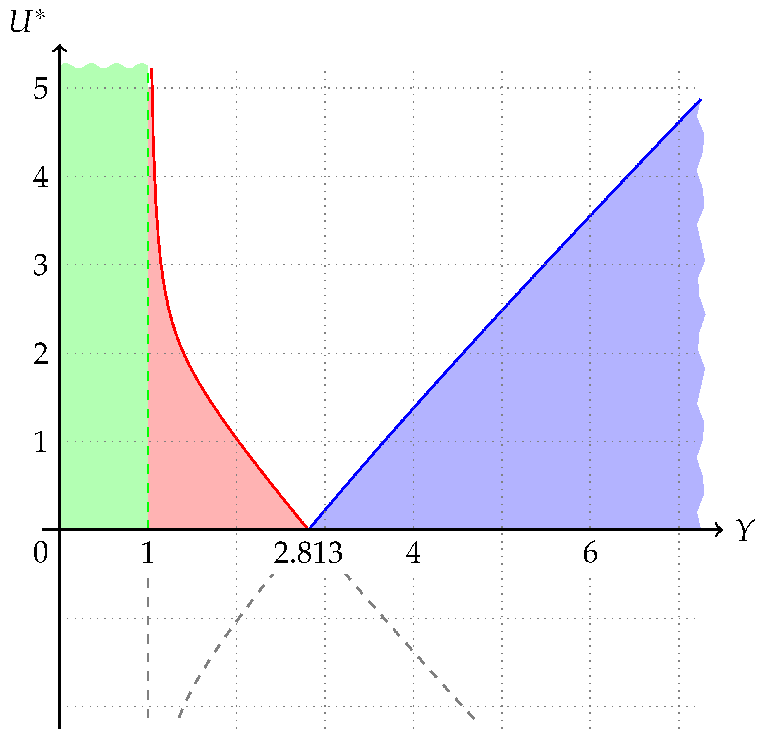
$$0<U^{*}<{\displaystyle \frac{|Y^3-2Y^2-3Y+2|}{\sqrt{Y^4-1}}}.$$

(31)

For the stripe $0<Y<1$, any number satisfies this constraint. In this case, $\mathcal{B}$ can take both positive and negative values, and the wave numbers are:

$$\delta ={\displaystyle \frac{1}{\mathcal{A}-{\tilde{\sigma }}_1}},k=\pm \mathcal{B}-{\tilde{\sigma }}_2.$$

(32)

For $Y>1$, the denominator in Equation (31) increases monotonically without singularities, while the numerator is zero at $Y\approx 2.813$. This splits the region $Y>1$ into two parts. The resulting three regions of the feasible set $U^{*}\left(Y\right)$ are shown in Figure 2.

Let us illustrate the solution by graphical representation of the wave numbers k and $\delta$ and let $s=2$. Then, the wave numbers under consideration are functions of the two variables, Y and $U^{*}$. The obtained graphical representations are given as two-dimensional surfaces in isometric projection.

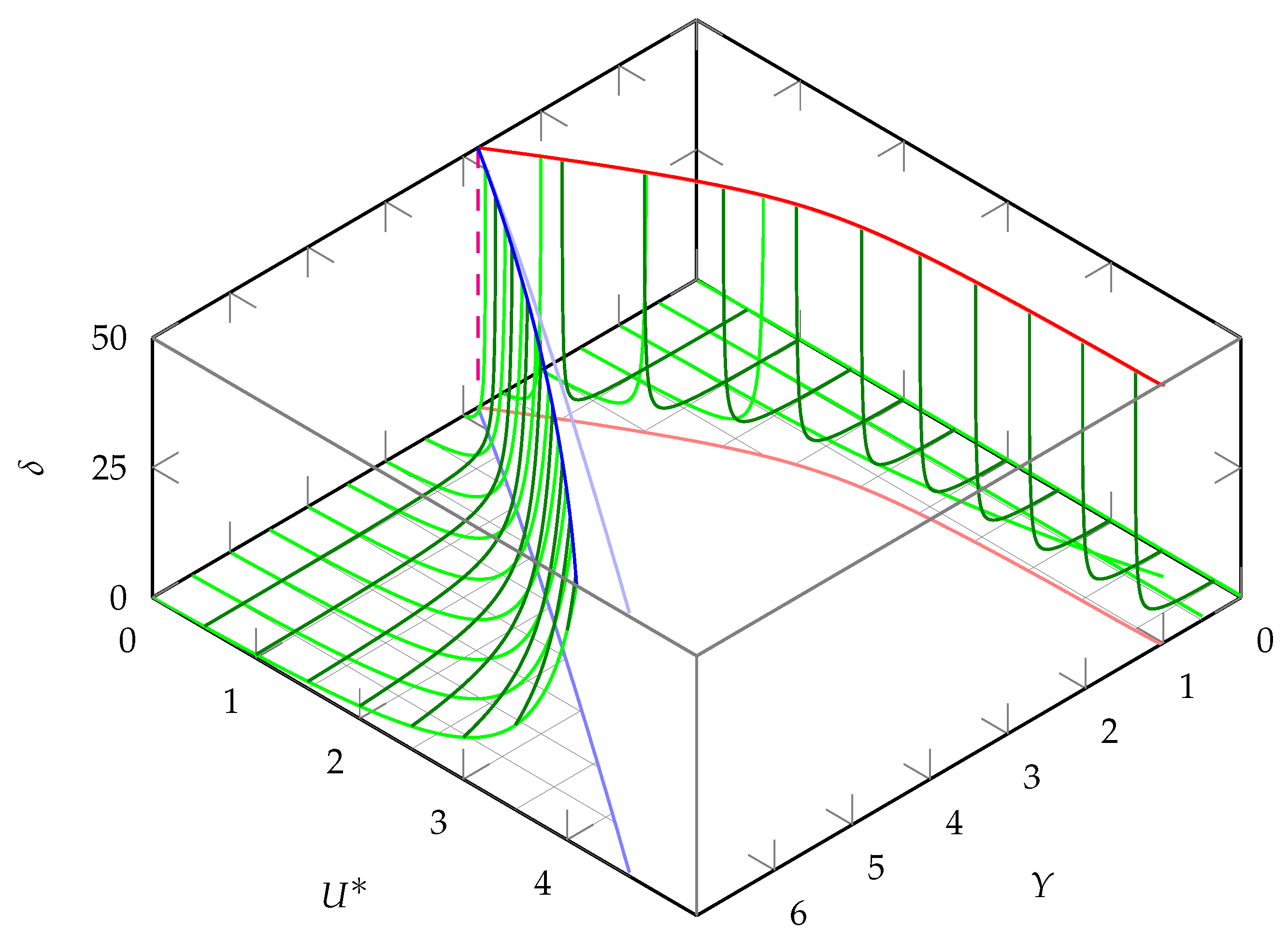
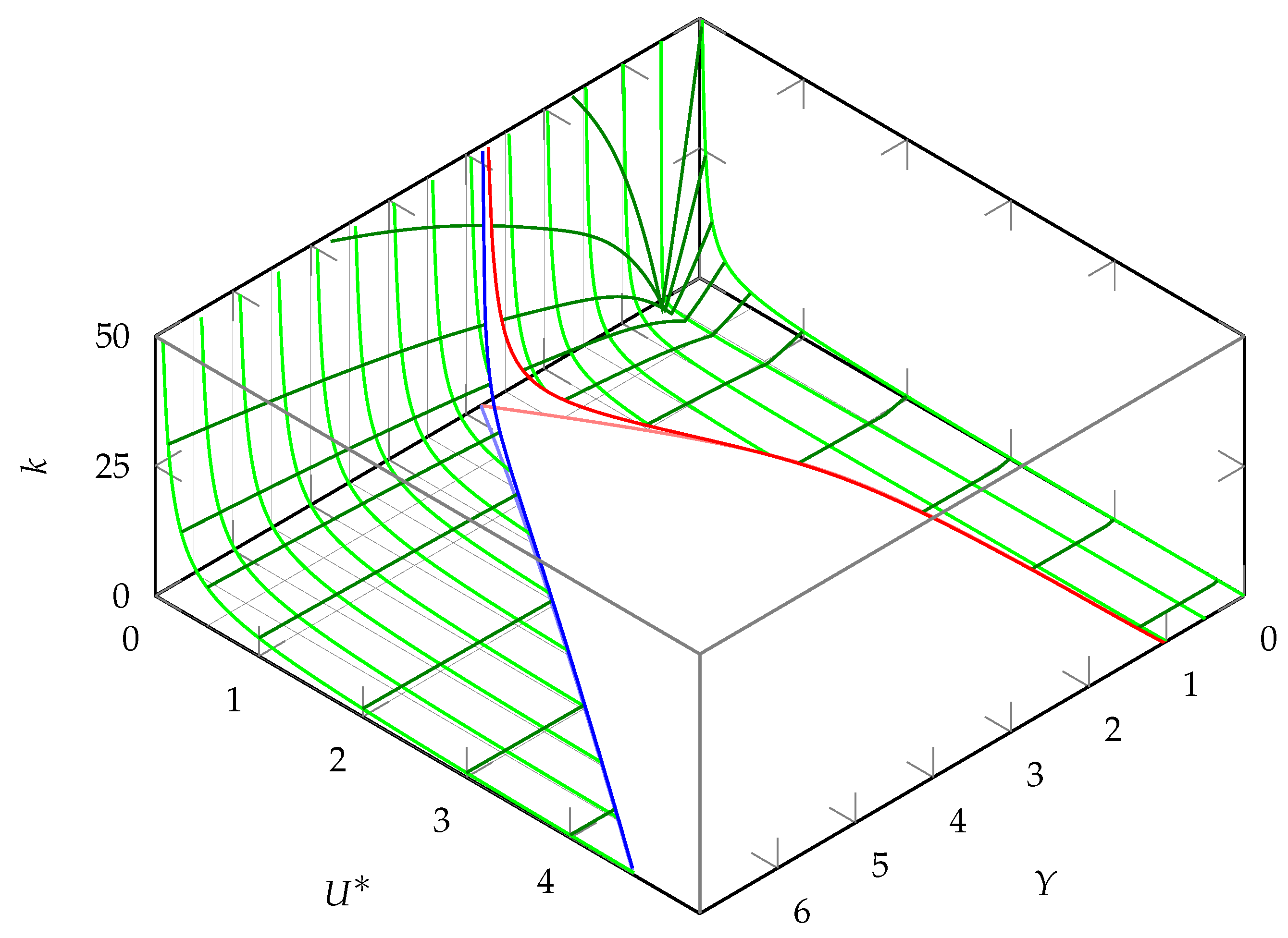
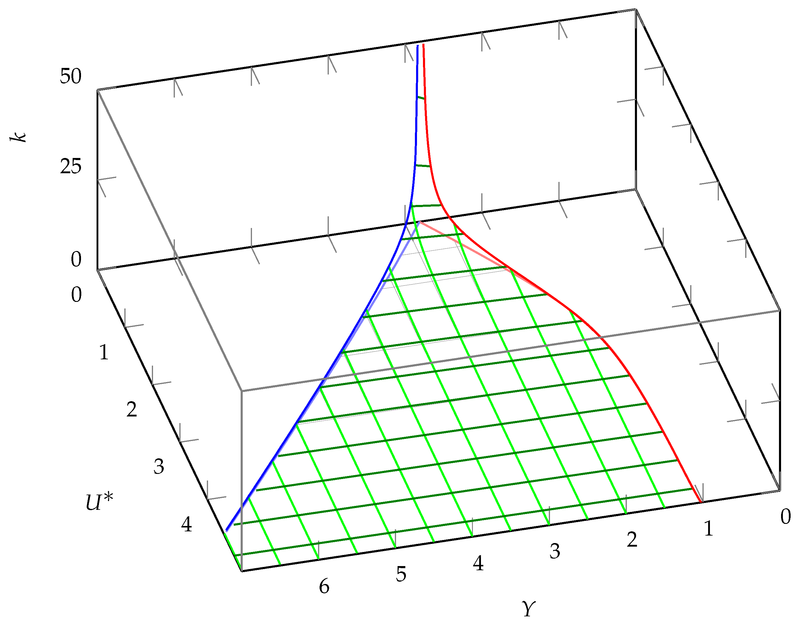
In the case of media injection, $U^{*}>0$. The first root ${\tilde{\chi }}_1$ is discarded and the second root has $\Re {\tilde{\chi }}_2={\tilde{\sigma }}_1-\mathcal{A}$, which yields the condition (31) for $Y>1$; for $0<Y<1$, any positive $U^{*}$ is feasible. The functions of wave numbers are given by Equation (32) with a positive sign at $\mathcal{B}$. This case is shown in Figure 3 and Figure 4 for $\delta$ and k, respectively.

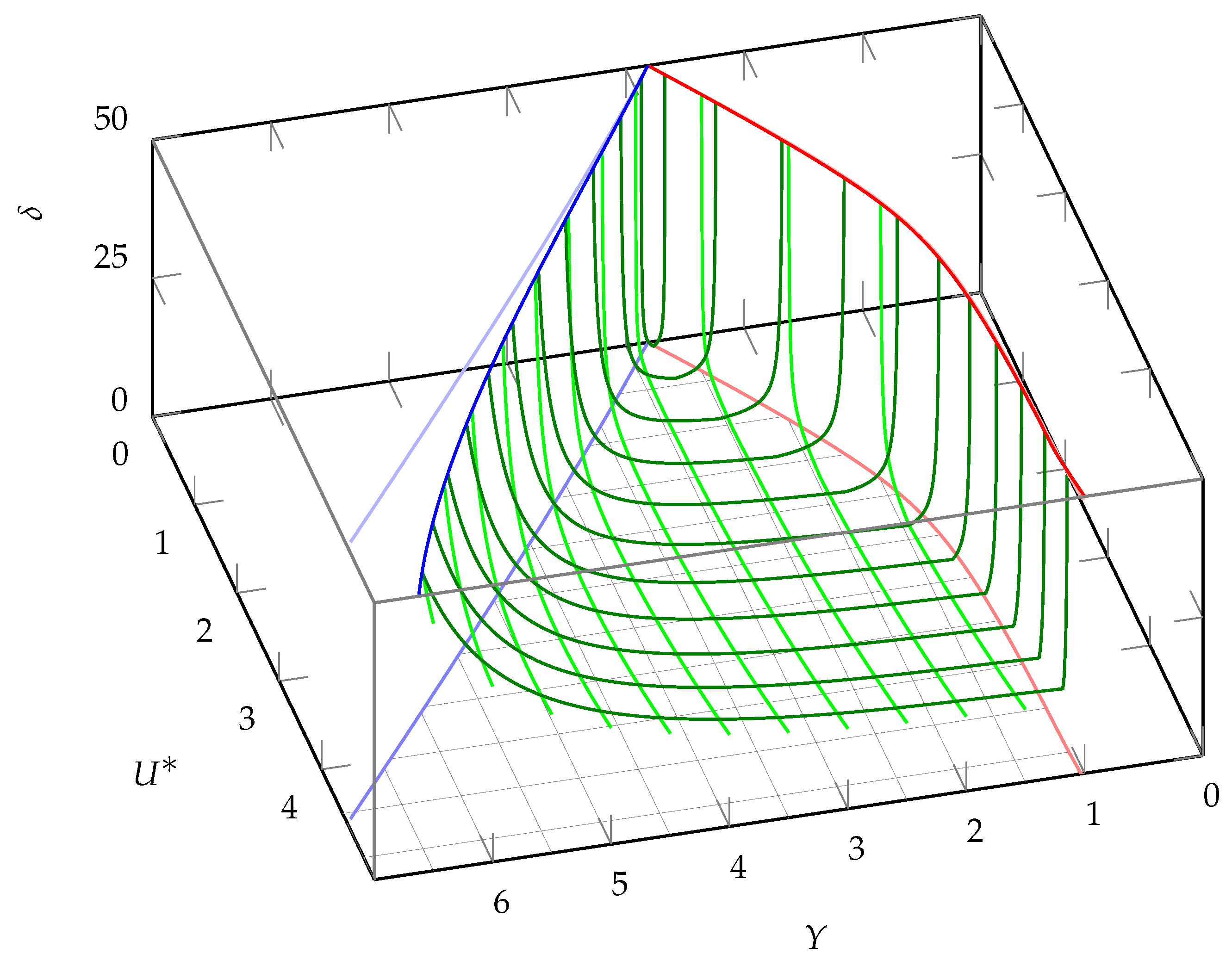
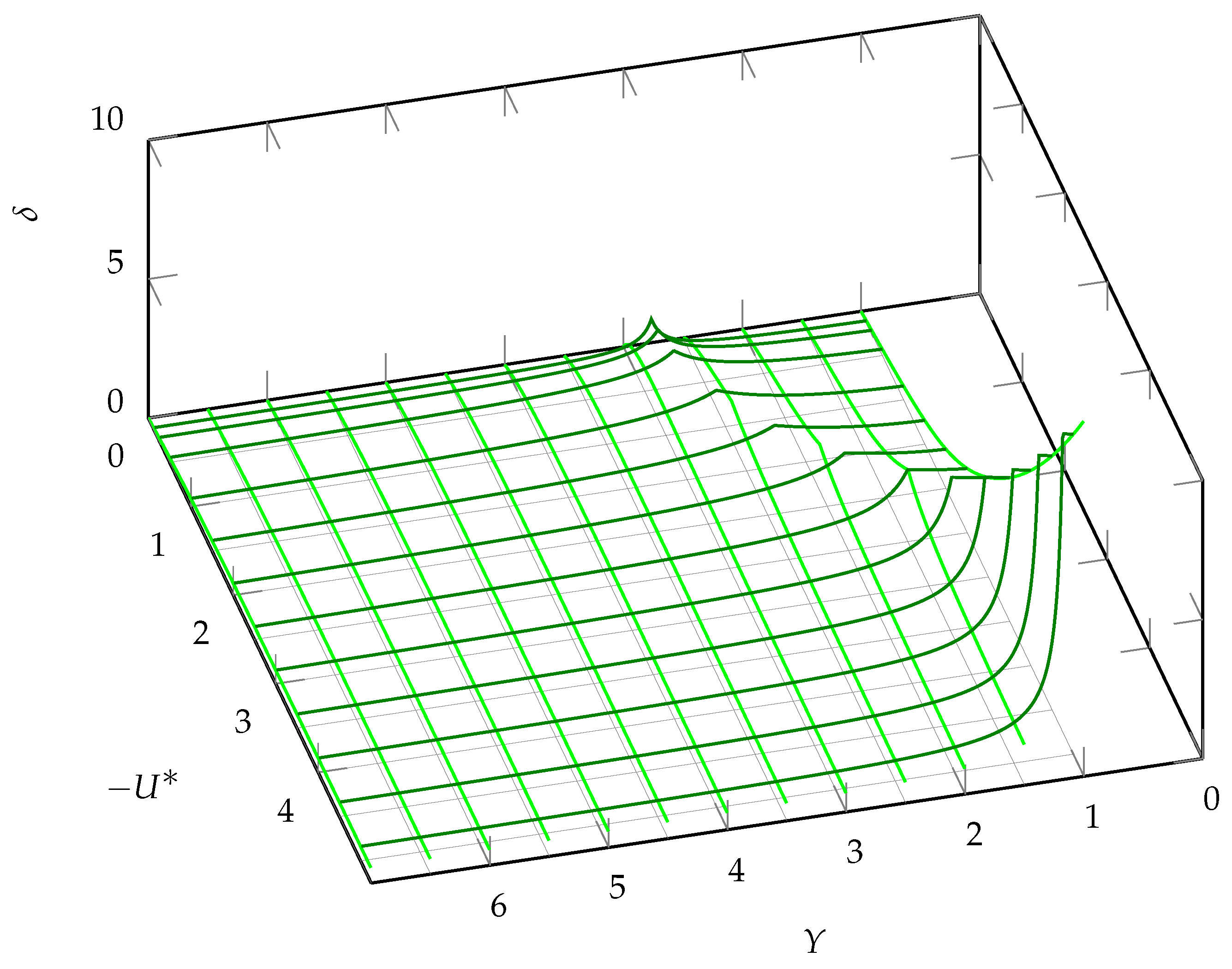
For the case of media suction, $U^{*}<0$, there are two roots. The fist one has $\Re {\tilde{\chi }}_1=-{\tilde{\sigma }}_1+\mathcal{A}$, which gives condition

$$U^{*}>{\displaystyle \frac{|Y^3-2Y^2-3Y+2|}{\sqrt{Y^2-1}}}$$

and there are no oscillations for $Y<1$. Wave numbers obey the same law (32). This case is illustrated in Figure 5 and Figure 6 for $\delta$ and k, respectively.

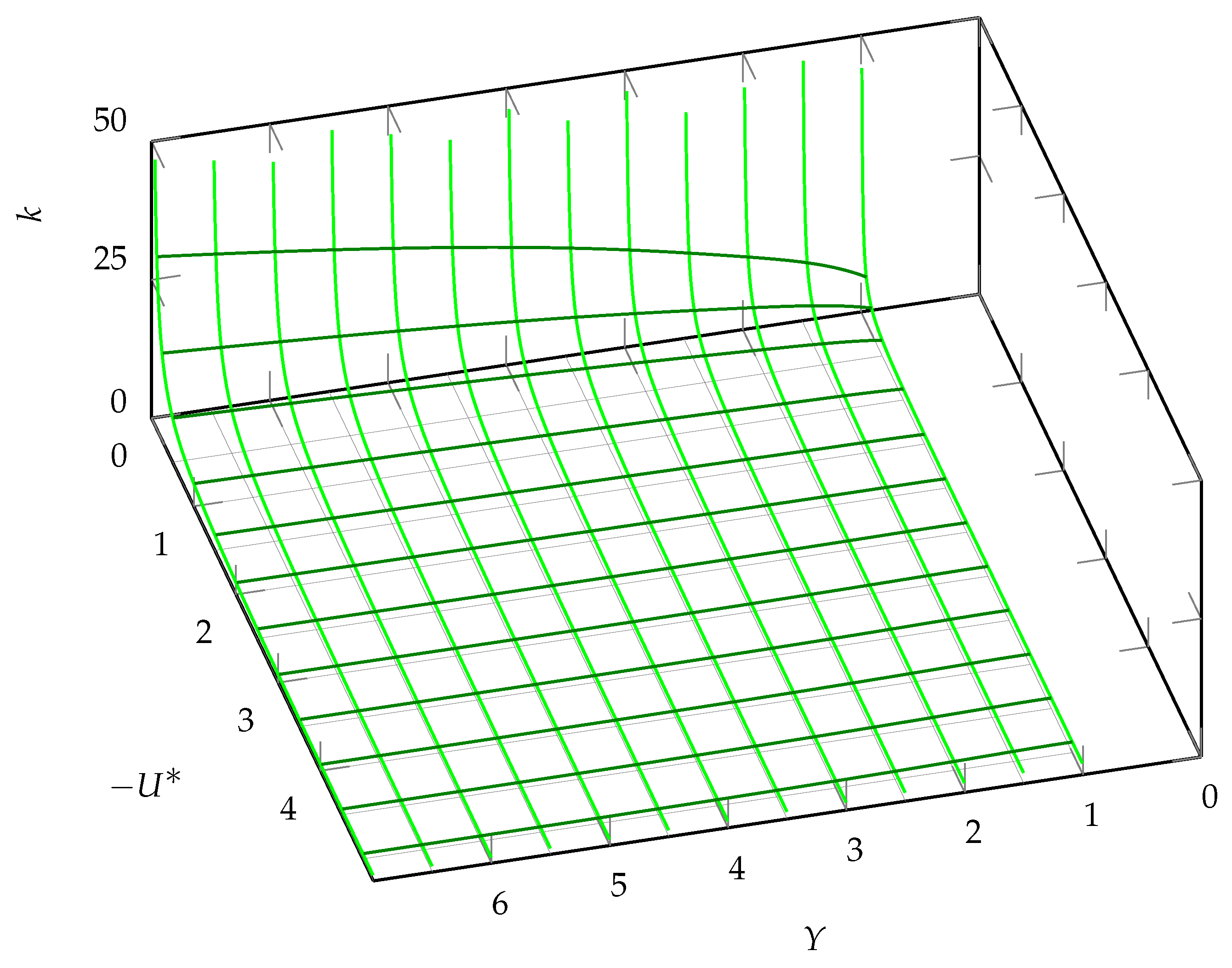
The second root in the case of suction has $\Re {\tilde{\chi }}_2=-{\tilde{\sigma }}_1-\mathcal{A}$, which is always below zero. Thus, the oscillations occur at any $U^{*}<0$, $Y>1$ and

$$\delta ={\displaystyle \frac{1}{\mathcal{A}+{\tilde{\sigma }}_1}},k=\mathcal{B}+{\tilde{\sigma }}_2.$$

This case is presented in Figure 7 and Figure 8 for $\delta$ and k, respectively.

5. Conclusions

The evolution of the flow of a viscous, incompressible, electrically conductive fluid in the presence of a magnetic field has been studied under the influence of suddenly initiated longitudinal oscillations of the plate and transverse fluid flow. The full equation of magnetic induction was used, i.e., energy dissipation due to the flow of electric currents was taken into account. No restrictions were initially imposed on the nature of the movement of the plate. Exact solutions to three-dimensional nonstationary equations of magnetohydrodynamics have been found. The velocity field and the induced magnetic field in the flow have been determined. The solution has been obtained through the Mellin integral containing the parameters of the system. The velocity field has been presented in the form of a superposition of plane waves propagating along the $Oy$ axis, the amplitudes of which decayed exponentially.

A special case of the oscillatory motion of the plate, which generated wave processes in the fluid, was considered. We have shown that, for some frequency intervals of plate oscillations, wave processes become impossible. In other words, for a large number of MHD problems, one can always select the necessary values of the specified parameters of the model to predict or obtain certain effects. So, in cosmology, planets rotate around their axes, which are inclined at various angles to the plane of their ecliptic.. Considering various planets, one can explain the discrepancies in their behaviors caused by different inclinations. Similar situations occur in the motion of spacecraft and aviation technology, as well as in the design of centrifuges, liquid-filled gyroscopes, and in fields such as geophysics, astrophysics, and marine physics. Therefore, the presented study and the solution found are of interest to a wide physics audience.

References

1. Alfvén, H. Existence of electromagnetic–hydrodynamic waves. Nature 1942, 150, 405–406. [Google Scholar] [CrossRef]
2. Gaifullin, A.M.; Nakrokhin, S.A. Compressible gas flow past a plate with upstream-moving surface. Fluid Dyn. 2021, 56, 45–49. [Google Scholar] [CrossRef]
3. Gaifullin, A.M.; Zhvick, V.V. The connection of the asymptotics of the far field of a jet with the velocity profile at an orifice. Dokl. Phys. 2020, 65, 387–389. [Google Scholar] [CrossRef]
4. Gaifullin, A.M.; Zhvik, V.V. Nonlocal conservation law in a free submerged jet. Comput. Math. Math. Phys. 2021, 61, 1630–1639. [Google Scholar] [CrossRef]
5. Dimitrieva, N.F. Stratified flow structure near the horizontal wedge. Fluid Dyn. 2019, 54, 940–947. [Google Scholar] [CrossRef]
6. Gavrikov, M.B. Two-Fluid Electromagnetic Hydrodynamics; URSS–Krasand: Moscow, Russia, 2018; Available online: https://www.rfbr.ru/library/books/2591/ (accessed on 25 December 2024). (In Russian)
7. Dimitrieva, N.F. Calculation of nonuniform fluid flows in a gravity field. In Proceedings of the International Conference: Topical Problems of Fluid Mechanics 2020, Prague, Czech Republic, 19–21 February 2020; Šimurda, D., Bondár, T., Eds.; Institute of Thermomechanics, Czech Academy of Sciences: Prague, Czech Republic, 2020; pp. 48–55. [Google Scholar] [CrossRef]
8. Chashechkin, Y.D. Differential fluid mechanics—Basis of the theory of flows with combustion. J. Phys. Conf. Ser. 2021, 1891, 012023. [Google Scholar] [CrossRef]
9. Ermakov, M.K. Modeling of vortex flow with a funnel based on the matrix method. In Proceedings of the 12th International Conference/School of Young Scientists: Waves and Vortices in Complex Media, Moscow, Russia, 1–3 December 2021; ISPOprint: Moscow, Russia, 2021; pp. 110–113. Available online: https://ipmnet.ru/en/conf/ (accessed on 25 December 2024). (In Russian).
10. Chashechkin, Y.D. Evolution of the fine structure of the matter distribution of a free-falling droplet in mixing liquids. Izv. Atmos. Ocean. Phys. 2019, 55, 285–294. [Google Scholar] [CrossRef]
11. Chashechkin, Y.D. Conventional partial and complete solutions of the fundamental equations of fluid mechanics in the problem of periodic internal waves with accompanying ligaments generation. Mathematics 2021, 9, 586. [Google Scholar] [CrossRef]
12. Poddubnyi, I.I.; Razuvanov, N.G. Investigation of hydrodynamics and heat transfer at liquid metal downflow in a rectangular duct in a coplanar magnetic field. Therm. Engin. 2016, 63, 89–97. [Google Scholar] [CrossRef]
13. Landau, L.D.; Lifshitz, E.M. Electrodynamics of Continuous Media; Pergamon Press Ltd./Elsevier Ltd.: Oxford, UK, 1984; Chapter VIII. [Google Scholar] [CrossRef]
14. Slezkin, N.A. Dynamics of a Viscous Incompressible Fluid; GITTL [State Publisher of Technical-Theoretical Literature]: USSR, 1955; Available online: http://booksshare.net/books/physics/slezkin-na/1955/files/dinamikavyazkoynesjimaemoyjidkosti1955.pdf (accessed on 25 December 2024). (In Russian)
15. Thornley, C. On stokes and Rayleigh layers in a rotating system. Quart. J. Mech. Appl. Math. 1968, 21, 451–461. [Google Scholar] [CrossRef]
16. Gupta, A.S. Ekman layer on a porous plate. Phys. Fluids 1972, 15, 930–941. [Google Scholar] [CrossRef]
17. Gurchenkov, A.; Yalamov, Y.I. Non-steady-state flow at a porous plate with blowing (suction) of the medium. J. Appl. Mech. Tech. Phys. 1980, 21, 488–491. [Google Scholar] [CrossRef]
18. Kholodova, E.S. Mathematical Modeling and Analysis of Flows and Waves in Rotating and Electrically Conductive Liquid Media. Ph.D. Thesis, Saint Petersburg State University, Saint Petersburg, Russia, 2019. [Google Scholar]
19. Gurchenkov, A.A. Nonstationary flow of a viscous incompressible electrically conductive fluid on a rotating plate. Fluid Dyn. 2021, 56, 943–953. [Google Scholar] [CrossRef]
20. Colombo, S.; Lavoine, J. Transformations de Laplace et de Mellin. Formulaires. Mode d’utilisation; Gauthier-Villars: Paris, France, 1972; Available online: http://www.numdam.org/item/?id=MSM_1972__169__1_0 (accessed on 25 December 2024).
21. Korn, G.A.; Korn, T.M. Mathematical Handbook for Scientists and Engineers; McGraw-Hill, Inc.: New York, NY, USA, 1968; Available online: https://archive.org/details/mathematicalhand0000korn_s8w4 (accessed on 25 December 2024).
Figure 1. Schematic geometry of the problem. See text for details.
Physics 07 00001 g001
Figure 2. Regions of solution on the (Y U * )-plane, where Y is a dimensionless frequency variable (28) and U * is a dimensionless injection velocity (30).
Physics 07 00001 g002
Figure 3. Wave surfaces of function δ ( U * , Y ) , case of injection. Pale red and pale blue lines on the (Y U * )-plane indicate the boundaries of the regions in Figure 2 shown with same colors. The upper pale blue line denotes the projection of the region drawn for clarity. The bright red and bright blue lines represent the intersection of the δ ( Y , U * ) surface with the δ = 50 plane. The bright green curves correspond to the lines of constant Y and the dark green curves represent the lines of constant U * .
Physics 07 00001 g003
Figure 4. Wave surfaces of function k ( U * , Y ) , case of injection. Pale red and pale blue lines on the (Y U * )-plane indicate the boundaries of the regions in Figure 2 shown with same colors. The upper pale blue line denotes the projection of the region drawn for clarity. The bright red and bright blue lines in Figure 4 depict the intersection of the k ( Y , U * ) surface with the region given by Equation (31). The bright green curves correspond to the lines of constant Y and the dark green curves represent the lines of constant U * .
Physics 07 00001 g004
Figure 5. Wave surfaces of function δ ( U * , Y ) , case of suction for root χ ˜ 1 . Pale red and pale blue lines on the (Y U * )-plane indicate the boundaries of the regions in Figure 2 shown with same colors. The upper pale blue line denotes the projection of the region drawn for clarity. The bright red and bright blue lines represent the intersection of the δ ( Y , U * ) surface with the δ = 50 plane. The bright green curves correspond to the lines of constant Y and the dark green curves represent the lines of constant U * .
Physics 07 00001 g005
Figure 6. Wave surfaces of function k ( U * , Y ) , case of suction for root χ ˜ 1 . Pale red and pale blue lines on the (Y U * )-plane indicate the boundaries of the regions in Figure 2 shown with same colors. The upper pale blue line denotes the projection of the region drawn for clarity. The bright red and bright blue lines in Figure 4 depict the intersection of the k ( Y , U * ) surface with the region given by Equation (31). The bright green curves correspond to the lines of constant Y and the dark green curves represent the lines of constant U * .
Physics 07 00001 g006
Figure 7. Wave surfaces of function δ ( U * , Y ) , case of suction for root χ ˜ 2 . See text for details. The bright green curves correspond to the lines of constant Y and the dark green curves represent the lines of constant U * .
Physics 07 00001 g007
Figure 8. Wave surfaces of function k ( U * , Y ) , case of suction for root χ ˜ 2 . See text for details. The bright green curves correspond to the lines of constant Y and the dark green curves represent the lines of constant U * .
Physics 07 00001 g008
Disclaimer/Publisher’s Note: The statements, opinions and data contained in all publications are solely those of the individual author(s) and contributor(s) and not of MDPI and/or the editor(s). MDPI and/or the editor(s) disclaim responsibility for any injury to people or property resulting from any ideas, methods, instructions or products referred to in the content.