Chemically Reactive Micropolar Hybrid Nanofluid Flow over a Porous Surface in the Presence of an Inclined Magnetic Field and Radiation with Entropy Generation

Abstract

The present study investigates the entropy generation of chemically reactive micropolar hybrid nanoparticle motion with mass transfer. Magnetic oxide (Fe₃O₄) and copper oxide (CuO) nanoparticles were mixed in water to form a hybrid nanofluid. The governing equations for velocity, concentration, and temperature are transformed into ordinary differential equations along with the boundary conditions. In the fluid region, the heat balance is kept conservative with a source/sink that relies on the temperature. In the case of radiation, there is a differential equation along with several characteristic coefficients that transform hypergeometric and Kummer’s differential equations by a new variable. Furthermore, the results of the current problem can be discussed by implementing a graphical representation with different factors, namely the Brinkman number, porosity parameter, magnetic field, micropolar parameter, thermal radiation, Schmidt number, heat source/sink parameter, and mass transpiration. The results of this study are presented through graphical representations that depict various factors influencing the flow profiles and physical characteristics. The results reveal that an increase in the magnetic field leads to a reduction in velocity and entropy production. Furthermore, temperature and entropy generation rise with a stronger radiation parameter, whereas the Nusselt number experiences a decline. This study has several industrial applications in technology and manufacturing processes, including paper production, polymer extrusion, and the development of specialized materials.

1. Introduction

Magnetic field fluid flow, and magnetohydrodynamic fluids in particular, have revolutionized various industries with their unique property of changing viscosity in response to a magnetic field. These viscous fluids are utilized in automotive systems for improved shock absorbers and dampers, in aerospace for adaptive wings, and in civil engineering for seismic dampers that protect structures during earthquakes. Additionally, magnetohydrodynamics is integral in medical devices for targeted drug delivery and in consumer electronics for haptic feedback systems. The versatility and rapid responsiveness of magnetohydrodynamics continue to inspire innovative applications across multiple fields. Due to these applications, many studies are devoted to investigations of magnetic fields. Reference [1] studied the Soret effect resulting from mixed convection on unstable magnetic flow across a vertical plate that is semi-infinitely permeable with heat absorption. Reference [2] studied the impact of time on a rotary magnetic refrigerator’s performance between the fluid flow profile and magnetic field profile. Reference [3] studied magnetic nanofluids under various alternating magnetic fields in terms of pressure drop and energy transfer performance. Reference [4] studied the spectral approach for the impact of magnetic field heat transfer in laminar fluid flow. Reference [5] studied the impact mechanism of the magnetic field on microstructure spot welds of aluminum resistance. Reference [6] studied a complex variety of transport processes used to statistically illustrate the impact of magnetic fields on controlling the transport of nanoparticle-based blood flow.

The Brinkman ratio is a dimensionless number that plays a main role in the study of fluid flow through porous media. It bridges the gap between Darcy’s law for slow, viscous flow and the Stokes equation for faster, inertial flows. By analyzing the Brinkman ratio, engineers can optimize filtration systems, enhance oil recovery methods, and improve the design of various industrial processes where fluid flow through porous structures is critical. This ratio is particularly useful in predicting the transition from purely viscous to inertial flow regimes, providing valuable insights for fluid dynamics research. Due to these applications, many investigations have studied Brinkman’s number. Reference [7] studied the impact of Brinkman flow on fractured walls and investigated it using a semi-analytical model. Reference [8] studied the electromagnetohydrodynamic behavior of a third-grade Newtonian liquid flow past parallel plates with electric fields. Reference [9] explored the influence of a Brinkman ratio on the thermophoresis translational motion of a spherical particle. References [10,11,12] studied the computational analysis of the properties of the Brinkman ratio and heat transfer in a decaying whirling flow.

A porous medium refers to the complex phenomenon of fluid flow through materials with interconnected void spaces, such as sand packs or fused Pyrex glass, where there are no clear-cut flow paths. Porous flows have applications in nuclear waste disposal technologies. Due to this application, many investigations have studied porous media. Reference [13] studied the impact of particle bridging and exclusion, as well as how particle size largely governs suspended particle behavior. Reference [14] studied the impact of flow rate and pore-scale heterogeneity on repeating two-phase liquid flow in microfluidic materials. Reference [15] studied the simulation of particle flow dynamics and its impact on mass transfer in permeable media. Reference [16] studied the variations in porosity that have an impact on the stability analysis of a homogenous fluid movement past a Brinkman permeable medium. References [17,18] studied the volume average, which is largely used to quantitatively analyze heat flow in a porous medium.

The interplay of chemical reactions and fluid flow is a cornerstone of process engineering, profoundly impacting the design and operation of reactors. It is fascinating how the rate of a chemical reaction can be influenced by the flow characteristics of the reactants, such as turbulence and mixing efficiency. This synergy is crucial in optimizing processes like combustion, polymerization, and waste treatment, ensuring efficiency and sustainability in industrial operations. Due to these applications, many investigations have studied chemical reaction parameters. Reference [19] studied the influence of chemical reactions on the magnetohydrodynamic fluid flow. Reference [20] studied the dynamics of magnetic nanofluid flow through a nonlinear porous stretched sheet. Reference [21] studied the stagnation point flows and slip effects of an upper-confected Maxwell fluid flowing over a stretched sheet. Reference [22] studied entropy generation produced with the aid of thermodynamic studies on energy expression with heat creation. References [23,24] studied the mathematical model for the hydrodynamic transport of reactive species undergoing chemical reactions with flowing blood.

Micropolar fluids, characterized by their microstructure, offer a more nuanced model of fluid dynamics by accounting for the rotational effects of fluid particles. This advanced approach has been instrumental in enhancing our understanding of various phenomena, from the behavior of anisotropic fluids and liquid crystals to the complexities of biological and environmental flows. The applications of micropolar theory extend to engineering and technology, providing valuable insights into the mechanics of fluids at microscale levels, which is critical for the development of efficient systems in fields such as biomedical engineering and nanotechnology. Due to these applications, many investigations have studied micropolar flow. Reference [25] studied the applications for mass and heat transfer in magnetohydrodynamic micropolar flows, including heat exchangers. Reference [26] studied the impact of various magnetic nanoparticles with micropolar fluid with the influence of a slip across a stretched sheet. References [27,28] explored the impact of a magnetic field on a biporous membrane’s hydrodynamic permeability about a micropolar liquid flow utilizing four broadly known cell models. Studies [29,30,31,32,33,34] explored the thermal transfer of a revolving, dusty micropolar liquid flow that is suspended in conducting dust particles over a stretched sheet of velocity. References [35,36,37,38,39,40,41,42,43,44,45,46] made in-depth investigations in the area of nanofluid flows subject to different physicochemical effects, including boiling, condensation, porosity, instability of different natures, and so on.

Inspired by the aforementioned discoveries and applications, the present paper studies the impact of radiation and an inclined magnetic field on the chemically reactive ferro hybrid nanofluid flow across permeable stretching/shrinking surfaces. To note is that there is a lack of study on ferro hybrid nanofluids under the conditions of a magnetic field and radiation with permeable media. The novelty of the present problem is examining the influence of a magnetic field and radiation and entropy generation analysis over ferro hybrid nanofluid flow. Similarity transformation is used to reduce the governing equations of the problem into a system of nonlinear ordinary differential equations, and current research illustrates that the temperature, velocity, and concentration are solved by the analytical method to obtain the exact solution and express the solution domain in terms of hypergeometric functions and the discussed results of porous media, mass transpiration, Schmidt number, skin friction, and Nusselt number. The results of the current study can be used in applications like the development of efficient fuel cells and the polymer industry with respect to stretching/shrinking sheets.

2. Model, Key Equations, and Solutions

Let us consider a permeable stretching or shrinking surface that is passed by an inclined magnetohydrodynamic boundary layer flow. The stretched sheet is considered to have a linear velocity, and the stretching/shrinking constant $\alpha$ [44] is positive for stretching and negative for shrinking sheets. Magnetic oxide (Fe₃O₄) and Cupric oxide (CuO) nanoparticles are mixed in water to form a nanofluid. The x-axis goes along the stretching or shrinking sheet, whereas the y-axis is normal to it; thermal radiation, Joule heating, and heat source sink effects are added to the temperature, and chemical reactions are added to the concentration equation. The sheet with a constant wall temperature is considered, and a magnetic field is applied to the flow with the inclined angle $\tau ={45}^{°}$. Figure 1 is the schematic representation of the fluid flow.

2.1. Restrictions and Assumptions

Our investigation is restricted to the following highlights and assumptions:

• Considered is an incompressible ferro-hybrid nanofluid with laminar flow.
• Considered are thermal radiation, heat source/sink, chemical reaction and Joule heating effects.
• Considered is a Newtonian base fluid water with magnetic oxide (Fe₃O₄) and cupric oxide (CuO) nanoparticles immersed.
• The flow is organized by the stretching of the surface, and with a negligible term of pressure gradient i.e., $\nabla p=0$.
• Assumed is steady incompressible movement, i.e., ${\displaystyle \frac{\partial u}{\partial t}}=0$, where u is the velocity and t denotes the time.
• Assumed is a surface stretching velocity $u_w\left(x\right)=bx$.

2.2. Governing Equations

The governing equations are [1,6,31]

$${\displaystyle \frac{\partial u}{\partial x}}+{\displaystyle \frac{\partial v}{\partial y}}=0,$$

(1)

$$u{\displaystyle \frac{\partial u}{\partial x}}+v{\displaystyle \frac{\partial u}{\partial y}}=\left[{\displaystyle \frac{{\mu }_{\mathrm{eff}}}{{\rho }_{\mathrm{hnf}}}}+{\displaystyle \frac{\vartheta }{{\rho }_{\mathrm{hnf}}}}\right]{\displaystyle \frac{{\partial }^{2}u}{\partial y^2}}+{\displaystyle \frac{\vartheta }{{\rho }_{\mathrm{hnf}}}}{\displaystyle \frac{\partial N}{\partial y}}-{\displaystyle \frac{{\sigma }_{\mathrm{hnf}}}{{\rho }_{\mathrm{hnf}}}}{\sin }^2\tau B_o^{2}u-{\displaystyle \frac{{\mu }_{\mathrm{hnf}}}{{\rho }_{\mathrm{hnf}}{k}^{*}}}u,$$

(2)

$$u{\displaystyle \frac{\partial N}{\partial x}}+v{\displaystyle \frac{\partial N}{\partial y}}={\displaystyle \frac{{\chi }^{*}}{{\rho }_{\mathrm{hnf}}j}}{\displaystyle \frac{{\partial }^{2}N}{\partial y^2}}-{\displaystyle \frac{\vartheta }{{\rho }_{\mathrm{hnf}}j}}\left[2N+{\displaystyle \frac{\partial u}{\partial y}}\right],$$

(3)

$$u{\displaystyle \frac{\partial T}{\partial x}}+\mathrm{v}{\displaystyle \frac{\partial T}{\partial y}}={\displaystyle \frac{{\kappa }_{\mathrm{hnf}}}{{(\rho c_p)}_{\mathrm{hnf}}}}{\displaystyle \frac{{\partial }^{2}T}{\partial y^2}}+\left[{\displaystyle \frac{{\mu }_{\mathrm{eff}}+\vartheta }{{(\rho c_p)}_{\mathrm{hnf}}}}\right]{\left[{\displaystyle \frac{\partial u}{\partial y}}\right]}^2-{\displaystyle \frac{1}{{(\rho c_p)}_{\mathrm{hnf}}}}{\displaystyle \frac{\partial {\mathrm{q}}_{\mathrm{r}}}{\partial y}}+{\displaystyle \frac{{\sigma }_{\mathrm{hnf}}}{{(\rho c_p)}_{\mathrm{hnf}}}}{\sin }^2\left(\tau \right)B_0^2{u}^2+{\displaystyle \frac{Q(T-T_{\infty })}{{(\rho c_p)}_{\mathrm{hnf}}}},$$

(4)

$$u{\displaystyle \frac{\partial C}{\partial x}}+v{\displaystyle \frac{\partial C}{\partial y}}=D_b{\displaystyle \frac{{\partial }^{2}C}{\partial y^2}}-{\mathrm{Cr}}^{*}(C-C_{\infty })$$

(5)

where $j$ is reference length, spin gradient viscosity modeled as $\chi *=\left({\mu }_{\mathrm{eff}}+{\displaystyle \frac{\vartheta }{2}}\right)j.$ $\mu$ is dynamic viscosity, ${\mu }_{\mathrm{eff}}$ is effective viscosity, $\vartheta$ is vortex viscosity, here u and v are the velocities parallel to the x and y axes, ρ is the density, N is the microrotation angular velocity, $c_p$ is the specific heat, $\kappa$ is the thermal conductivity of the fluid, σ is the electrical conductivity, and dynamic viscosity is given by μ. B_o is the magnetic field of strength, Q is the heat source/sink coefficient. T is the local temperature, N is micro rotation component, C is the concentration, k* is the permeability of porous medium, D_b is the mass diffusivity, and Cr* is the chemical reaction parameter. The subscripts “hnf” denotes the “hybrid nanofluid” and the infinity symbol denotes the free steam. ${\mathrm{q}}_{\mathrm{r}}$ is radiative heat flux.

Here, the Rosseland estimation (for radiation flux) is characterized by [1,6,31]

$${\mathrm{q}}_{\mathrm{r}}=-{\displaystyle \frac{4{\sigma }^{*}}{3{\epsilon }^{*}}}{\displaystyle \frac{\partial T^4}{\partial y}},$$

(6)

where σ* is the Stefan–Boltzmann constant and ε* the mean absorption parameter.

The heat fluctuations between the local temperature T and free steam T_∞ are negligible, since the Taylor succession expansion of $T^4$ about $T_{\infty }$ excludes higher-order factors:

$$T^4\cong 4T_{\infty }^{3}T-3T_{\infty }^4.$$

(7)

The radiation term in Equation (4) is developed as

$$u{\displaystyle \frac{\partial T}{\partial x}}+\mathrm{v}{\displaystyle \frac{\partial T}{\partial y}}={\displaystyle \frac{1}{{(\rho c_p)}_{\mathrm{hnf}}}}\left({\kappa }_{\mathrm{hnf}}+{\displaystyle \frac{4{\sigma }^{*}{T}_{\infty }^3}{3{\epsilon }^{*}}}\right){\displaystyle \frac{{\partial }^{2}T}{\partial y^2}}+\left[{\displaystyle \frac{{\mu }_{\mathrm{eff}}+\vartheta }{{(\rho c_p)}_{\mathrm{hnf}}}}\right]{\left[{\displaystyle \frac{\partial u}{\partial y}}\right]}^2+{\displaystyle \frac{{\sigma }_{\mathrm{hnf}}}{{(\rho c_p)}_{\mathrm{hnf}}}}{\sin }^2\left(\tau \right)B_0^2{u}^2+{\displaystyle \frac{Q(T-T_{\infty })}{{(\rho c_p)}_{\mathrm{hnf}}}}.$$

(8)

2.3. Boundary Conditions (BCs)

For the suggested model the boundary conditions (BCs) are [1,6,31]

$$\begin{array}{l}u=u_w(x)=b x,\hspace{1em}\hspace{1em}\hspace{1em}v=v_w,\hspace{1em}\hspace{1em}\hspace{1em}\mathrm{at}\hspace{1em}y=0,\\ u\to 0,\hspace{1em}\hspace{1em}\hspace{1em}\hspace{1em}\hspace{1em}\hspace{1em}\hspace{1em}\hspace{1em}\hspace{1em}\hspace{1em}\hspace{1em}\hspace{1em} \mathrm{as}\hspace{1em}y\to \infty ;\end{array}$$

(9)

$$\begin{array}{l}N=-n{\displaystyle \frac{\partial u}{\partial y}},\hspace{1em}\hspace{1em}\hspace{1em}\hspace{1em}\hspace{1em}\hspace{1em}\hspace{1em}\hspace{1em}\hspace{1em}\mathrm{at}\hspace{1em}y=0,\\ N\to 0, \hspace{1em}\hspace{1em}\hspace{1em}\hspace{1em}\hspace{1em}\hspace{1em}\hspace{1em}\hspace{1em}\hspace{1em}\hspace{1em}\mathrm{as}\hspace{1em}y\to \infty ;\end{array}$$

(10)

$$\begin{array}{l}T=T_w=T_{\infty }+A{\left({\displaystyle \frac{x}{l}}\right)}^2(\mathrm{PST}), -Z{\displaystyle \frac{\partial T}{\partial y}}=q_w=B{\left({\displaystyle \frac{x}{l}}\right)}^2(\mathrm{PHF}),\hspace{1em}\mathrm{at}\hspace{1em}y=0,\\ T\to T_{\infty },\hspace{1em}\hspace{1em}\hspace{1em}\hspace{1em}\hspace{1em}\hspace{1em}\hspace{1em}\hspace{1em}\hspace{1em}\hspace{1em}\hspace{1em}\hspace{1em}\hspace{1em}\hspace{1em}\hspace{1em}\hspace{1em}\hspace{1em}\hspace{1em}\hspace{1em}\hspace{1em}\hspace{1em}\mathrm{as}\hspace{1em}y\to \infty ,\\ -D\left({\displaystyle \frac{\partial C}{\partial y}}\right)=m_w=F{\left({\displaystyle \frac{x}{l}}\right)}^2,\hspace{1em}\hspace{1em}\hspace{1em}\hspace{1em}\hspace{1em}\hspace{1em}\hspace{1em}\hspace{1em}\hspace{1em}\hspace{1em}\hspace{1em}\hspace{1em}\hspace{1em}\hspace{1em}\mathrm{at}\hspace{1em}y=0,\\ C\to C_{\infty },\hspace{1em}\hspace{1em}\hspace{1em}\hspace{1em}\hspace{1em}\hspace{1em}\hspace{1em}\hspace{1em}\hspace{1em}\hspace{1em}\hspace{1em}\hspace{1em}\hspace{1em}\hspace{1em}\hspace{1em}\hspace{1em}\hspace{1em}\hspace{1em}\hspace{1em}\hspace{1em}\hspace{1em}\mathrm{as}\hspace{1em}y\to \infty ;\end{array}$$

(11)

where S is mass transpiration. Equation (10) uses a boundary parameter n that ranges from 0 to 1. The value of n = 0 in this case indicates weak concentrations of microelements at the sheet and corresponds to the state in which they are unable to rotate at the stretching sheet. Microelement concentration is weak in the case n = ½, and turbulent boundary layer flows are in the case of n = 1 [38,39,40]. A, B, D and F are constants respectively, and $q_w,m_w$ are dimensionless heat and mass flux, respectively. “PST” and “PHF” stand for prescribed surface temperature and prescribed heat flux, respectively.

2.4. Similarity Transformation

Let us introduce the following dimensionless and similarity terms used in the governing Equations (2)–(5) and convert them into ordinary differential equations [1,6,31]:

$$\eta ={(a/\nu )}^{1/2}y, u=ax{f}^{\prime }\left(\eta \right), v=-{\left(a\nu \right)}^{1/2}f\left(\eta \right),$$

(12)

$$N={\left(a/\nu \right)}^{1/2}axg\left(\eta \right), \theta \left(\eta \right)={\displaystyle \frac{T-T_{\infty }}{T_w-T_{\infty }}}, \phi \left(\eta \right)={\displaystyle \frac{C-C_{\infty }}{C_w-C_{\infty }}},$$

(13)

with the functions g(η) and f(η) to be determined. The variable a denotes the stretching coefficient. The prime denotes the η–derivative.

Using Equation (13), the governing boundary layer Equations (2)–(5) read

$$\begin{array}{l}\left(\Lambda +K\right)f^{‴}\left(\eta \right)-A_2\left({\left(f^{\prime }\left(\eta \right)\right)}^2-f\left(\eta \right)f^{″}\left(\eta \right)\right)+K{g}^{\prime }\left(\eta \right)\\ -A_{3}M{\sin }^2\tau f^{\prime }\left(\eta \right)-A_{1}Q*f^{\prime }\left(\eta \right)=0,\end{array}$$

(14)

$$\left(\Lambda +{\displaystyle \frac{K}{2}}\right)g^{″}\left(\eta \right)+A_2\left(g^{\prime }\left(\eta \right)f\left(\eta \right)-g\left(\eta \right)f^{\prime }\left(\eta \right)\right)-K\left(f^{″}\left(\eta \right)-2g\left(\eta \right)\right),$$

(15)

PHF:

$$\begin{array}{l}\left(A_4+\mathrm{Nr}\right){\delta }^{″}\left(\eta \right)+A_5\mathrm{Pr}f\left(\eta \right){\delta }^{\prime }\left(\eta \right)-A_5\mathrm{Pr}(2f^{\prime }(\eta )-\mathrm{Ni})\delta (\eta )\\ =-\mathrm{Pr}{\mathrm{Ec}}_2[(A_1+K)f^{″}\left(\eta \right)+A_{3}M {\sin }^2\left(\tau \right){\left(f^{\prime }(\eta )\right)}^2],\end{array}$$

(16)

PST:

$$\begin{array}{l}\left(A_4+\mathrm{Nr}\right){\theta }^{″}\left(\eta \right)+A_5\mathrm{Pr}f\left(\eta \right){\theta }^{\prime }\left(\eta \right)-A_5\mathrm{Pr}(2f^{\prime }(\eta )-\mathrm{Ni})\theta (\eta )\\ =-\mathrm{Pr}{\mathrm{Ec}}_1[(A_1+K)f^{″}\left(\eta \right)+A_{3}M {\sin }^2\left(\tau \right){\left(f^{\prime }(\eta )\right)}^2],\end{array}$$

(17)

$${\phi }^{″}\left(\eta \right)-\mathrm{Sc}f\left(\eta \right){\phi }^{\prime }\left(\eta \right)-\mathrm{Sc}\left(2f^{\prime }\left(\eta \right)-{\mathrm{Kc}}^{*}\right)\phi \left(\eta \right)=0,$$

(18)

where δ(η) denotes the temperature for PHF case, $\theta \left(\eta \right)$ denotes temperature for PST case, $\phi \left(\eta \right)$ denotes the concentration, $K={\displaystyle \frac{\vartheta }{{\mu }_f}}$ is the micro-rotation parameter,

$Q*={\displaystyle \frac{{\nu }_f}{k^{*}a}}$ is the porosity parameter,

$A_1={\displaystyle \frac{{\mu }_{\mathrm{hnf}}}{{\mu }_f}},$ $A_2={\displaystyle \frac{{\rho }_{\mathrm{hnf}}}{{\rho }_f}},$ $A_3={\displaystyle \frac{{\sigma }_{\mathrm{hnf}}}{{\sigma }_f}},$ $A_4={\displaystyle \frac{{\kappa }_{\mathrm{hnf}}}{{\kappa }_f}},$

$A_5={\displaystyle \frac{{\left(\rho c_p\right)}_{\mathrm{hnf}}}{\rho c_{\mathit{pf}}}}$ are constants,

$M={\displaystyle \frac{{\sigma }_f{B}_0^2}{{\rho }_{f}a}}$ is the magnetic field parameter,

$\mathrm{Nr}={\displaystyle \frac{16{\sigma }^{*}{T}_{\infty }^3}{3{\kappa }_f{\epsilon }^{*}}}$ denotes the radiation parameter,

${\mathrm{Ec}}_1=\left({\displaystyle \frac{a^2{l}^2}{{\mathrm{Ac}}_{\mathrm{p}}}}\right)$ and ${\mathrm{Ec}}_2=\left({\displaystyle \frac{a^2{l}^{2}Z}{{\mathrm{Bc}}_{\mathrm{p}}}}\sqrt{{\displaystyle \frac{a}{\nu }}}\right)$ are the Eckert numbers, with characteristic length l,

$\mathrm{Pr}={\displaystyle \frac{{\nu }_f{\left(\rho c_p\right)}_f}{{\kappa }_f}}$ is the Prandtl number,

${\mathrm{Kc}}^{*}={\displaystyle \frac{{\mathrm{Cr}}^{*}}{a}}$ is the chemical reaction parameter,

$\mathrm{Ni}={\displaystyle \frac{Q_0}{a{(\rho C_p)}_f}}$ is the heat source/sink,

$\mathrm{Sc}={\displaystyle \frac{{\nu }_f}{D_b}}$ denotes the Schmidt number,

$\Lambda ={\displaystyle \frac{{\mu }_{\mathrm{eff}}}{{\mu }_{\mathrm{f}}}}$ denotes the Brinkman ratio.

The modified boundary conditions read

$$\begin{array}{l}f\left(0\right)=S,\hspace{1em}{f}^{\prime }\left(0\right)={\displaystyle \frac{b}{a}}=\alpha ,\hspace{1em}g\left(0\right)=-n{f}^{″}\left(0\right),\hspace{1em}\theta \left(0\right)=1,\hspace{1em}\phi \left(0\right)=1,\hspace{1em}\mathrm{as}\hspace{1em}\eta =0,\\ f^{\prime }\left(\eta \right)\to 0,\hspace{1em}g\left(\eta \right)\to 0,\hspace{1em}\theta \left(\eta \right)\to 0,\hspace{1em}\phi \left(\eta \right)\to 0,\hspace{1em}\hspace{1em}\hspace{1em}\hspace{1em}\hspace{1em}\hspace{1em}\hspace{1em}\hspace{1em}\hspace{1em} \mathrm{at}\hspace{1em}\eta \to \infty .\end{array}$$

(19)

Skin friction coefficient C_fx and the local Nusselt number N_ux are calculated as

$$\begin{array}{l}{\mathrm{C}}_{\mathrm{fx}}={\displaystyle \frac{{\left[\left({\mu }_{\mathrm{eff}}+\vartheta \right)\frac{\partial u}{\partial y}+\vartheta N\right]}_{y=0}}{{\rho }_{\mathrm{hnf}}{u}_w^2}} \\ {\mathrm{N}}_{\mathrm{ux}} = -{\left[{\displaystyle \frac{x}{{\kappa }_f\left(T_w-T_{\infty }\right)}}\left({\kappa }_{\mathrm{hnf}}{\displaystyle \frac{\partial T}{\partial y}}+{\displaystyle \frac{4\sigma *}{3\epsilon *}}{\displaystyle \frac{\partial T^4}{\partial y}}\right)\right]}_{y=0}.\end{array}$$

(20)

Dimensionless forms are

$$\begin{gathered} {\mathrm{Re}}_x^{1/2}{C}_{\mathrm{fx}}=\left[{\displaystyle \frac{1+\Lambda (1-n)K}{\Lambda }}\right]{\displaystyle \frac{f^{″}(0)}{A_2}}, \\ {\mathrm{Re}}_x^{-1/2}{\mathrm{N}}_{\mathrm{ux}}=-\left[A_4+\mathrm{Nr}\right]{\theta }^{\prime }(0), \end{gathered}$$

(21)

where ${\mathrm{Re}}_x=a{x}^2/\nu$ is local Reynolds number.

3. Solution of the Velocity Equation

From BCs, the solution for angular and velocity equations are

$$f(\eta )=S+{\displaystyle \frac{\alpha }{\beta }}(1-e^{-\beta \eta }), g(\eta )={\displaystyle \frac{\alpha \beta }{2}}{e}^{-\beta \eta },$$

(22)

with β represents the solution of root or solution parameter.

Substituting Equation (22) into Equation (14), one gets

$$(K+2\Lambda ){\beta }^2-2S\beta A_2-2(Q*A_1+\alpha A_2+M{\sin }^2\tau A_3)=0.$$

(23)

Solving Equation (21), the solution roots $\beta$ are as follows:

$$\beta ={\displaystyle \frac{2S{A}_2\pm \sqrt{4S^2{A}_2^2-4(K+2\Lambda )(-2Q*A_1-2\alpha A_2-2M{\sin }^2\tau A_3)}}{2(K+2\Lambda )}}.$$

(24)

Thus, the solution of Equation (14) concerning BCs (19) is given by

$$\begin{array}{l}f(\eta )=S+{\displaystyle \frac{2\alpha (K+2\Lambda )}{2S{A}_2\pm \sqrt{4S^2{A}_2^2-4(K+2\Lambda )(-2Q*A_1-2\alpha A_2-2M{\sin }^2\tau A_3)}}}\\ \times \left(1-\exp \left[-{\displaystyle \frac{2S{A}_2\pm \sqrt{4S^2{A}_2^2-4(K+2\Lambda )(-2Q*A_1-2\alpha A_2-2M{\sin }^2\tau A_3)}}{2(K+2\Lambda )}}\eta \right]\right),\end{array}$$

(25)

$$\begin{array}{l}g(\eta )={\displaystyle \frac{1}{2}} {\displaystyle \frac{2\alpha (K+2)}{2S{A}_2\pm \sqrt{4S^2{A}_2^2-4(K+2\Lambda )(-2Q*A_1-2\alpha A_2-2M{\sin }^2\tau A_3)}}}\\ \times \exp \left[-{\displaystyle \frac{2S{A}_2\pm \sqrt{4S^2{A}_2^2-4(K+2\Lambda )(-2Q*A_1-2\alpha A_2-2M{\sin }^2\tau A_3)}}{2(K+2\Lambda )}}\eta \right].\end{array}$$

(26)

Differentiating Equation (25) once, one finds the velocity profile:

$$f^{\prime }(\eta )=\alpha \exp \left[-{\displaystyle \frac{2S{A}_2\pm \sqrt{4S^2{A}_2^2-4(K+2\Lambda )(-2Q*A_1-2\alpha A_2-2M{\sin }^2\tau A_3)}}{2(K+2\Lambda )}}\eta \right].$$

4. Analytic Solution for the Temperature Equation

To solve the energy Equation (16) for the PST case, let us choose the variable t as f[17,31,43].

$$t={\displaystyle \frac{-\mathrm{Pr}}{{\beta }^2}}{e}^{-\beta \eta }, {\mathrm{Pr}}^{*}={\displaystyle \frac{\mathrm{Pr}}{{\beta }^2}}.$$

(27)

By using Equation (16), the energy equation reads

$$\begin{array}{l}\left(A_4+\mathrm{Nr}\right)t{\displaystyle \frac{{\partial }^2\theta }{\partial t^2}}+\left[\left(A_4+\mathrm{Nr}\right)-{\displaystyle \frac{\mathrm{Pr}}{\beta }}\left({\displaystyle \frac{A_{5}S\beta +A_5\alpha }{\beta }}\right)-A_5\alpha t\right]{\displaystyle \frac{\partial \theta }{\partial t}}\\ +\left(2A_5\alpha +{\displaystyle \frac{\mathrm{PrNi}}{{\beta }^{2}t}}\right)\theta (t)=-{\displaystyle \frac{{\alpha }^2{\beta }^2{\mathrm{Ec}}_1(A_{3}M {\sin }^2\left(\tau \right)+(A_1+K){\beta }^2)}{{\mathrm{Pr}}^{*}}}t.\end{array}$$

(28)

The following are the equivalent BCs

$$\theta \left(-{\displaystyle \frac{\mathrm{Pr}}{{\beta }^2}}\right)=1, \theta \left(0\right)=0.$$

(29)

Let us introduce particular integral and its t-derivatives:

$$\begin{array}{l}{\theta }_p(t)=A{t}^2,\\ {\theta }_p^{\prime }(t)=2At,\\ {\theta }_p^{″}(t)=2A.\end{array}$$

Equation (28) can be then rewritten as

$$\begin{array}{l}\left(A_4+\mathrm{Nr}\right)t{\theta }_p^{″}+\left[\left(A_4+\mathrm{Nr}\right)-{\displaystyle \frac{\mathrm{Pr}}{\beta }}\left({\displaystyle \frac{A_{5}S\beta +A_5\alpha }{\beta }}\right)-A_5\alpha t\right]{\theta }_p^{\prime }\\ +\left(2A_5\alpha +{\displaystyle \frac{\mathrm{PrNi}}{{\beta }^{2}t}}\right)\theta =-{\displaystyle \frac{{\alpha }^2{\beta }^2{\mathrm{Ec}}_1(A_{3}M {\sin }^2\left(\tau \right)+(A_1+K){\beta }^2)}{{\mathrm{Pr}}^{*}}}t,\end{array}$$

(30)

Solving Equation (30), one finds

$${\theta }_p(t)={\displaystyle \frac{-{\alpha }^2{\beta }^2{\mathrm{Ec}}_1(A_{3}M {\sin }^2\left(\tau \right)+(A_1+K){\beta }^2)}{{\mathrm{Pr}}^{*}\left[4\left(A_4+\mathrm{Nr}\right)-\frac{2\mathrm{Pr}}{\beta }\left(\frac{A_{5}S\beta +A_5\alpha }{\beta }\right)+\frac{\mathrm{PrNi}}{{\beta }^2}\right]}}{t}^2.$$

(31)

Let us take the homogeneous component of Equation (30) and proceed to determine the complementary function θ_c(p):

$$\begin{array}{l}\left(A_4+\mathrm{Nr}\right)t{\displaystyle \frac{{\partial }^2\theta }{\partial t^2}}+\left[\left(A_4+\mathrm{Nr}\right)-{\displaystyle \frac{\mathrm{Pr}}{\beta }}\left({\displaystyle \frac{A_{5}S\beta +A_5\alpha }{\beta }}\right)-A_5\alpha t\right]{\displaystyle \frac{\partial \theta }{\partial t}}\\ +\left(2A_5\alpha +{\displaystyle \frac{\mathrm{PrN}i}{{\beta }^{2}t}}\right)\theta (t)=0.\end{array}$$

(32)

Applying the Frobenius method, we expand

$$\theta ={\displaystyle \sum _{r=0}^{\infty }{a}_r{t}^{k+r}}, {\theta }^{\prime }={\displaystyle \sum _{r=0}^{\infty }{a}_r(k+r)t^{k+r-1}}, {\theta }^{″}={\displaystyle \sum _{r=0}^{\infty }{a}_r(k+r)(k+r-1)t^{k+r-1}}.$$

(33)

With hypergeometric series, one can substitute Equation (33) into Equation (32) to obtain

$${\theta }_c(t)=a_0{t}^{{\displaystyle \frac{1}{2}}\left[{\displaystyle \frac{\mathrm{Pr}}{\beta }}\left({\displaystyle \frac{A_{5}S\beta +A_5\alpha }{\beta }}\right)+D\right]}{}_1\mathrm{F}_1\left[a-2,1+A_7,A_5\alpha t\right],$$

(34)

where ₁F₁ represents the hypergeometric function.

The solution for temperature Equation (16) is calculated as

$$\theta \left(t\right)={\theta }_c(t)+{\theta }_p(t).$$

(35)

Substituting Equations (31) and (34) into Equation (35), one gets

$$\begin{array}{l}\theta (t)=a_0{t}^{{\displaystyle \frac{1}{2}}\left[{\displaystyle \frac{\mathrm{Pr}}{\beta }}\left({\displaystyle \frac{A_{5}S\beta +A_5\alpha }{\beta }}\right)+D\right]}{}_1\mathrm{F}_1 \left[a-2,1+A_7,A_5\alpha t\right]\\ -{\displaystyle \frac{{\alpha }^2{\beta }^2{\mathrm{Ec}}_1\left(A_{3}M {\sin }^2\left(\tau \right)+\left(A_1+K\right){\beta }^2\right)}{{\mathrm{Pr}}^{*}\left[4\left(A_4+Nr\right)-\frac{2\mathrm{Pr}}{\beta }\left(\frac{A_{5}S\beta +A_5\alpha }{\beta }\right)+\frac{\mathrm{PrNi}}{{\beta }^2}\right]}}{t}^2.\end{array}$$

(36)

The exact solution of the temperature equation for the PST case is

$$\begin{array}{l}\theta \left(\eta \right)={\displaystyle \frac{\frac{1+\mathrm{Pr}{\alpha }^2{\mathrm{Ec}}_1\left(A_{3}M {\sin }^2\left(\tau \right)+\left(A_1+K\right){\beta }^2\right)}{\overline{W}}}{{}_1\mathrm{F}_1 \left[\overline{a},1+A_7,-A_5\frac{\mathrm{Pr}}{{\beta }^2}\right]}}\exp \left[-\left({\displaystyle \frac{\mathrm{Pr}}{\beta }}\right)\left({\displaystyle \frac{A_{5}S\beta +A_5\alpha }{\beta }}\right){\displaystyle \frac{A}{\alpha }}\right]\\ \times {}_1\mathrm{F}_1\left[\overline{a},1+A_7,-\alpha {\displaystyle \frac{\mathrm{Pr}{e}^{-\beta \eta }}{{\beta }^2}}\right]{\displaystyle \frac{-{\alpha }^2\mathrm{Pr}{\mathrm{Ec}}_1\left(A_{3}M {\sin }^2\left(\tau \right)+\left(A_1+K\right){\beta }^2\right)}{\overline{W}}},\end{array}$$

(37)

where

$$\overline{a}=a+2, \overline{W}=4A-a_1+a_2,$$

$$A=\left(A_4+\mathrm{Nr}\right), A_7={\displaystyle \frac{\sqrt{a_1^2-4a^{2}A}}{A}},$$

$$a_1={\displaystyle \frac{\mathrm{Pr}}{\beta }}\left({\displaystyle \frac{A_{5}S\beta +A_5\alpha }{\beta }}\right), a_2={\displaystyle \frac{\mathrm{Pr}\mathrm{Ni}}{{\beta }^2}}.$$

To solve the energy Equation (17) for the PHF case, we chose variable t as follows

$$t={\displaystyle \frac{-\mathrm{Pr}}{{\beta }^2}}{e}^{-\beta \eta }, {\mathrm{Pr}}^{*}={\displaystyle \frac{\mathrm{Pr}}{{\beta }^2}}.$$

(38)

By using the Fibonacci series and Hypergeometric function, one gets

$$\begin{array}{l}\delta (t)=a_0{t}^{{\displaystyle \frac{1}{2}}\left[{\displaystyle \frac{\mathrm{Pr}}{\beta }}\left({\displaystyle \frac{A_{5}S\beta +A_5\alpha }{\beta }}\right)+D\right]}{}_1\mathrm{F}_1 \left[a-2,1+A_7,A_5\alpha t\right]\\ -{\displaystyle \frac{{\alpha }^2{\beta }^2{\mathrm{Ec}}_2\left(A_{3}M {\sin }^2\left(\tau \right)+\left(A_1+K\right){\beta }^2\right)}{{\mathrm{Pr}}^{*}\left[4\left(A_4+\mathrm{Nr}\right)-\frac{2\mathrm{Pr}}{\beta }\left(\frac{A_{5}S\beta +A_5\alpha }{\beta }\right)+\frac{\mathrm{PrNi}}{{\beta }^2}\right]}}{t}^2.\end{array}$$

(39)

The modified BCs read

$${\delta }^{\prime }\left(-{\displaystyle \frac{\mathrm{Pr}}{{\beta }^2}}\right)=-{\displaystyle \frac{1}{{\mathrm{Pr}}^{*}\beta }}, \delta \left(0\right)=0 .$$

(40)

The solution for the PHF case is calculated as follows

$$\begin{gathered} \delta \left(\eta \right)={\displaystyle \frac{1}{\beta }}+{\displaystyle \frac{2{\alpha }^{2}E{c}_2\mathrm{Pr}\left(A_{3}M {\sin }^2\left(\tau \right)+(A_1+K){\beta }^2\right)}{\overline{W}}}\left\{{\displaystyle \frac{1}{2}}\left(\left({\displaystyle \frac{\mathrm{Pr}}{\beta }}\right)\left({\displaystyle \frac{A_{5}S\beta +A_5\alpha }{\beta }}\right)\right) {}_1\mathrm{F}_1\left[\overline{a},1+A_7,-\alpha {\displaystyle \frac{\mathrm{Pr}}{{\beta }^2}}\right]\right\} \\ \times \exp \left[-\left({\displaystyle \frac{\mathrm{Pr}}{\beta }}\right)\left({\displaystyle \frac{A_{5}S\beta +A_5\alpha }{\beta }}\right)+A_7\right]{}_1\mathrm{F}_1 \left[\overline{a},1+A_7,-\alpha {\displaystyle \frac{\mathrm{Pr}{e}^{-\beta \eta }}{{\beta }^2}}\right]-{\displaystyle \frac{{\alpha }^2\mathrm{Pr}{\mathrm{Ec}}_2{A}_{3}M {\sin }^2\left(\tau \right)\left(A_1+K\right){\beta }^2}{\overline{W}}}{e}^{-2\beta \eta }. \end{gathered}$$

(41)

5. Analytic Solution for the Concentration Equation

We select the variable ${\mathrm{t}}_1$ as follows

$${\mathrm{t}}_1={\displaystyle \frac{-\mathrm{Sc}}{{\beta }^2}}{e}^{-\beta \eta }$$

(42)

to solve the concentration Equation (18).

Equation (42) is used to derive the concentration equation as

$${\mathrm{t}}_1{\displaystyle \frac{{\partial }^2\phi }{\partial {{\mathrm{t}}_1}^2}}+\left[1-C_1-\alpha {\mathrm{t}}_1\right]{\displaystyle \frac{\partial \phi }{\partial t}}+\left(2\alpha -{\displaystyle \frac{{\mathrm{Kc}}^{*}\mathrm{Sc}}{{\beta }^2{\mathrm{t}}_1}}\right)=0,$$

(43)

with $C_1=\left({\displaystyle \frac{\mathrm{Sc}(1+S)}{\beta }}\right)$.

The following are the equivalent BCs

$$\phi \left({\displaystyle \frac{\mathrm{Sc}}{{\beta }^2}}\right)=1,\phi (0)=0.$$

(44)

The solution of the concentration equation is then calculated as

$$\phi (\eta )={(e^{-\beta \eta })}^{{\displaystyle \frac{C_1+A_8}{2}}}{\displaystyle \frac{{}_1\mathrm{F}_1 \left[\frac{C_1+A_8}{2}-2A_8,1+A_8,\frac{-\mathrm{Sc}}{{\beta }^2}{e}^{-\beta \eta }\right]}{{}_1\mathrm{F}_1\left[\frac{C_1+b}{2}-2A_8,1+A_8,\frac{-\mathrm{Sc}}{{\beta }^2}\right]}},$$

(45)

where

$$C_1=\left({\displaystyle \frac{\mathrm{Sc}(1+S)}{\beta }}\right), A_8=\sqrt{C_1^2+4\mathrm{Sc}{\displaystyle \frac{{\mathrm{Kc}}^{*}}{{\beta }^2}}.}$$

6. Entropy Generation Analysis

The entropy generation of the micropolar hybrid nanofluid is calculated as [33,34]

$$\mathrm{Sg}={\displaystyle \frac{{\kappa }_{\mathrm{hnf}}}{T_{\infty }^2}}\left[1+{\displaystyle \frac{16\sigma *T_{\infty }^3}{3\epsilon *{\kappa }_f}}\right]{\left({\displaystyle \frac{\partial T}{\partial y}}\right)}^2+{\displaystyle \frac{\left({\mu }_{\mathrm{eff}}+\vartheta \right)}{T_{\infty }}}{\left({\displaystyle \frac{\partial u}{\partial y}}\right)}^2+{\displaystyle \frac{{\sigma }_{\mathrm{hnf}}}{T_{\infty }}}{\left(u \sin \left(\tau \right)B_0\right)}^2,$$

(46)

$$\mathrm{with} \mathrm{heat} \mathrm{transfer} \mathrm{irreversibility} {\displaystyle \frac{{\kappa }_{\mathrm{hnf}}}{T_{\infty }^2}}\left[1+{\displaystyle \frac{16\sigma *T_{\infty }^3}{3\epsilon *{\kappa }_f}}\right]{\left({\displaystyle \frac{\partial T}{\partial y}}\right)}^2,$$

(47)

$$\mathrm{fluid} \mathrm{friction} \mathrm{irreversibility} {\displaystyle \frac{\left({\mu }_{\mathrm{eff}}+\vartheta \right)}{T_{\infty }}}{\left({\displaystyle \frac{\partial u}{\partial y}}\right)}^2,$$

(48)

$$\mathrm{and} \mathrm{Joule} \mathrm{heating} \mathrm{irreversibility} {\displaystyle \frac{{\sigma }_{\mathrm{hnf}}}{T_{\infty }}}{\left(u \sin \left(\tau \right)B_0\right)}^2.$$

(49)

The entropy production rate is given by

$$\begin{array}{l}\mathrm{Ng}={\displaystyle \frac{{\nu }_f{T}_{\infty }}{b{\kappa }_f}}\mathrm{Sg}=\left(A_4+\mathrm{Nr}\right)\delta {\left({\theta }^{\prime }\right)}^2\\ +\mathrm{Br}\left[\left(\Lambda +K\right){\left(f^{″}\right)}^2+A_3 {\sin }^2\left(\tau \right)M{\left(f^{\prime }\right)}^2\right],\end{array}$$

(50)

where $\mathrm{Br}=\mathrm{Ec}\times \mathrm{Pr}$, and the temperature difference parameter is $\Delta ={\displaystyle \frac{T_w-T_{\infty }}{T_{\infty }}}$.

7. Results and Discussion

This paper studies the entropy generation of chemically reactive micropolar hybrid nanofluid flow with mass transfer. The results of the current problem can be discussed by implementing a graphical representation with different factors, namely, the Brinkman number, porosity parameter, magnetic field, micropolar parameter, thermal radiation, Schmidt number, heat source/sink, Brinkman mass suction/injection and radiation parameters are studied. Setting the numerical value of the Prandtl number Pr as 6.72 for water, and the range of parameters taken as $-3\le \alpha \le 3$, $-0.5\le S\le 5$, $0.1\le \Lambda \le 5$, $0.1\le M\le 4$, $0\le Br\le 3$, $0.5\le Q*\le 5$, $0.01\le \varphi <0.03$, $0\le \mathrm{Ni},\mathrm{Ec},K\le 5$, $0.1\le \mathrm{Nr}\le 5$, thermophysical properties are given in

Table 1. Thermophysical characteristics of hybrid nanofluids (HNFs) [31]. See text for details.

Characteristics of HNFs
Heat capacity    ${\displaystyle \frac{{(\rho C_p)}_{\mathrm{hnf}}}{{(\rho C_p)}_f}}=\left(1-{\varphi }_2\right)\left(1-{\varphi }_1+{\varphi }_1\left({\displaystyle \frac{{(\rho C_P)}_{s_1}}{{(\rho C_P)}_f}}\right)\right)+{\varphi }_2\left({\displaystyle \frac{{(\rho C_P)}_{s_2}}{{(\rho C_P)}_f}}\right)$,
Density        ${\rho }_{\mathrm{hnf}}=\left(1-{\varphi }_2\right)\left[\left(1-{\varphi }_1\right){\rho }_f+{\rho }_{s1}\right]+{\varphi }_2{\rho }_{s2}$,
Dynamic viscosity   ${\mu }_{\mathrm{hnf}}={\displaystyle \frac{{\mu }_f}{{\left(1-{\varphi }_1\right)}^{2.5}{\left(1-{\varphi }_2\right)}^{2.5}}}$,
Thermal conductivity  $\begin{array}{l}{\displaystyle \frac{{\kappa }_{\mathrm{hnf}}}{{\kappa }_f}}={\displaystyle \frac{{\kappa }_{s_2}+2{\kappa }_{\mathrm{nf}}+2{\varphi }_2({\kappa }_{s_2}-{\kappa }_f)}{{\kappa }_{s_2}+2{\kappa }_{\mathrm{nf}}-{\varphi }_2({\kappa }_{s_2}-{\kappa }_f)}}\\ {\displaystyle \frac{{\kappa }_{\mathrm{nf}}}{{\kappa }_f}}={\displaystyle \frac{{\kappa }_{s_1}+2{\kappa }_f+2{\varphi }_1({\kappa }_{s_1}-{\kappa }_f)}{{\kappa }_{s_1}+2{\kappa }_f-{\varphi }_1({\kappa }_{s_1}-{\kappa }_f)}}\end{array}$,
Electrical conductivity $\begin{array}{l}{\displaystyle \frac{{\sigma }_{\mathrm{hnf}}}{{\sigma }_f}}={\displaystyle \frac{{\sigma }_{s_2}+2{\sigma }_{\mathrm{nf}}+2{\varphi }_2({\sigma }_{s_2}-{\sigma }_f)}{{\sigma }_{s_2}+2{\sigma }_{\mathrm{nf}}-{\varphi }_2({\sigma }_{s_2}-{\sigma }_f)}}\\ {\displaystyle \frac{{\sigma }_{\mathrm{nf}}}{{\sigma }_f}}={\displaystyle \frac{{\sigma }_{s_1}+2{\sigma }_f+2{\varphi }_1({\sigma }_{s_1}-{\sigma }_f)}{{\sigma }_{s_1}+2{\sigma }_f-{\varphi }_1({\sigma }_{s_1}-{\sigma }_f)}}\end{array}$,

Here, ${\varphi }_1$ and ${\varphi }_2$ are the solid volume capacity, subscripts $s_1$ and $s_2$ denote nanoparticles Fe₃O₄ and CuO, subscript f denotes base fluid and “hnf” denotes hybrid nanofluid.

.

Table 2. Numerical quantities of fluid and nanoparticles [45,46]. See text for details.

Properties	H2O (Water)	Fe3O4 (Magnetic Oxide)	CuO (Copper Oxide)
$\sigma (\mathrm{S}/\mathrm{m})$	5.5 × 10−6	2.5 × 104	6.9 × 10−2
$\rho {(\mathrm{kgm}}^{-3})$	997.1	5180	6510
$C_p {(\mathrm{JkgK}}^{-1})$	4179	670	540
$\kappa {(\mathrm{WmK}}^{-1})$	0.613	9.7	18

represents the numerical quantities of fluid and nanoparticles.

Figure 2a,b portrays, respectively, the axial and angular velocities for various choices of the porosity parameter Q*. The solid and dashed lines denote the hybrid and nanofluid flows, respectively. Increasing the porosity parameter decreases the axial and angular velocity for stretching and shrinking boundaries. Physically, this is because the increase in the choices of the porosity parameter tends to lower the permeability of the porous media, imparting more resistance offered to the movement due to the permeable fiber, which leads to the deceleration in transport.

Figure 3a,b portrays, respectively, the axial and angular velocities for various choices of micropolar parameter K. Solid lines denote the hybrid nanofluid flow and the dashed line denotes the nanofluid flow. Increasing the K parameter increases the axial and angular velocities for stretching and shrinking boundaries. Physically, when the micropolar parameter grows, it indicates that the microstructure of freedom has a greater influence on fluid flow. This might increase the complexity of flow patterns and velocity profiles.

Figure 4a,b portrays, respectively, the axial and angular velocities for various choices of the magnetic field parameter M. The solid and dashed lines denote the hybrid and nanofluid flows, respectively. Increasing the magnetic field decreases the axial and angular velocity for stretching and shrinking boundaries. Physically, Lorentz’s force came to bear when a magnetohydrodynamics was imposed across the flow field. This force drags the fluid flow by cutting down its velocity.

Figure 5a,b represents, respectively, the axial and angular velocities for various choices of mass transpiration. The solid and dashed lines denote the hybrid and nanofluid flows, respectively. Increasing the mass transpiration decreases the axial and angular velocity for stretching and shrinking boundaries. Physically, with permeable boundaries, the fluid experiences higher viscosity and results in resistance to flow, which tends to reduce the velocity.

Figure 6a,b represents, respectively, the axial and angular velocities for various choices of the Brinkman number Λ. The solid and dashed lines denote the hybrid and nanofluid flows, respectively. Increasing the Brinkman number decreases the axial and angular velocity for stretching and shrinking boundaries. This is due to the physical impact of a Brinkman fluid, where a greater value of Brinkman fluid increases viscous forces in comparison to thermal forces. Therefore, the velocity of the fluid tends to decrease.

Figure 7a,b portrays the temperature for PST and PHF, respectively, for different choices of the Eckert number Ec. The solid and dashed lines denote the hybrid and nanofluid flows, respectively. Increasing the Ec increases the temperature of PST and PHF cases. This occurs because heat is generated in the fluid when the choice of Ec grows owing to frictional heating. Physically, the Ec is the ratio of kinetic energy to the specific enthalpy difference between the fluid and wall. As a result, a rise in Ec causes the conversion of kinetic energy into internal energy through effort against viscous fluid forces. As a result, raising Ec increases the temperature of the fluid.

Figure 8 represents the temperature of the PST case for different choices of heat source/sink Ni. The solid and dashed lines denote the hybrid and nanofluid flows, respectively. Increasing the heat source/sink increases the temperature of the PST case due to decaying the thickness of the thermal boundary layer. Physically this reveals the feature that an increase in the Ni parameter means an increase in the heat generated in the boundary layer, which tends to a greater temperature.

Figure 9a,b portrays the temperature of the PST and PHF cases, respectively, for different choices of the radiation parameter Nr. The solid and dashed lines denote the hybrid and nanofluid flows, respectively. Increasing the Nr increases the temperature of the PST and PHF cases. Physically, enhancing radiative characteristics encourages molecule mobility in the fluid, which leads to the conversion of heat energy through frequent collisions between nanoparticles when the surface wall is at both suction or injection and there is no permeability for both kinds of nanoparticles.

Figure 10a,b portrays the temperature of the PST and PHF cases, respectively, for different choices of magnetic field. The solid and dashed lines denote the hybrid and nanofluid flows, respectively. Increasing the magnetic parameter M increases the temperature of both the PST and PHF cases. Figure 10c represents the concentration for different values of the Schmidt number Sc. Increasing the Schmidt number decreases the concentration. Physically, enhancing radiative characteristics encourages molecule mobility in the fluid, which leads to the conversion of heat energy through frequent collisions between nanoparticles when the surface wall is at both suction or injection and there is no permeability for both kinds of nanoparticles.

Figure 11 represents the Nusselt number for various choices of the heat source/sink parameter Ni. The solid and dashed line denotes the hybrid and nanofluid flows, respectively. Increasing the Ni decreases the Nusselt number. In the case of a heat source and heat sink, it is hypothesized that more heat is produced inside the fluid. The heat produced within the fluid by the Ni parameter causes thermal diffusivity to increase and decrease the Nusselt number.

Figure 12 represents the Nusselt number Nu for various choices of the magnetic field. The solid and dashed line denotes the hybrid and nanofluid flows, respectively. Increasing the magnetic field decreases the Nusselt number. Physically, an increase in the magnetic field tends to decay temperature gradients, hence decreasing the Nusselt number.

Figure 13 represents the Nusselt number for various choices of the radiation parameter Nr. The solid and dashed line denote the hybrid and nanofluid flows, respectively. Increasing the radiation parameter decreases the Nusselt number. Physically, this is because the heat extraction and absorption terms of the nanoparticle intensify as the choices of the Nr parameter increase; as a result, the rate of heat transport raises.

Figure 14 represents the entropy production for various choices of the magnetic field parameter M. The solid and dashed lines denote the hybrid and nanofluid flows, respectively. Increasing the magnetic field decreases the entropy production. Physically, this can be explained through the feature that as M increases, the Lorentz resisting force also raises due to thermal convection. As M raises the entropy productions due to heat transfer irreversibility, this is resulting in the reduction of entropy production.

Figure 15 represents the entropy production for different choices of the Brickman number Br. Solid lines denote the hybrid nanofluid, and the dashed line denotes the nanofluid flow. Increasing the Br number increases the entropy production; an increase in the Br number means that a larger amount of heat has been produced through viscous dissipation. Therefore, raising the Br number raises the entropy production.

Figure 16 represents the entropy production for different choices of radiation number Nr. The solid and dashed lines denote the hybrid and nanofluid flows, respectively. Increasing the radiation number increases the entropy production. Physically, this is because as the Nr parameter ramps up, the fluid temperature decays, being emitted via radiation and hence results in lowering the unavailable energy, which tends to minimize the heat transfer irreversibility. Therefore, entropy production decreases as radiation increases.

Figure 17 represents the skin friction for various choices of the stretching/shrinking parameter α. Solid lines denote the hybrid nanofluid and the dashed lines denote the nanofluid flow. Increasing the stretching/shrinking parameter increases skin friction. Physically, as the surface stretches, the fluid particles near the surface are pulled along with it. This causes an increase in velocity gradient near the surface. A higher velocity gradient results in a stronger viscous force, leading to an increased skin friction.

Figure 18 represents the skin friction for different choices of the magnetic field parameter M. The solid and dashed lines denote the hybrid and nanofluid flows, respectively. Increasing the magnetic field increases skin friction. Physically, the reason for this behavior is that the Coriolis force affects the fluid motion, which gives an increase in the velocity gradients of the flows.

Figure 19a,b represents stream line graphs for two different values of the porosity parameter. Figure 19c,d represents the stream line graphs for two different values of the Brinkman ratio. Figure 19e,f represents the stream line graphs for two different values of magnetic field parameter.

8. Conclusions

In the present paper, the entropy generation of chemically reactive micropolar hybrid nanofluids with heat and mass transfer is discussed. The results of the current problem can be discussed by implementing a graphical representation with different factors, namely the Brinkman number, porosity parameter, magnetic field, micropolar parameter, thermal radiation, Schmidt number, heat source/sink, mass transpiration, and radiation parameter,

Table 3. Comparison of the present study and other related studies.

References		Value of Velocity Solution
Ref. [41] (1970)	Newtonian	$\beta =1$
Ref. [42] (1974)	Newtonian	$\beta = \sqrt{1+M}$
Ref. [43] (2022)	Non-Newtonian	$f\left(\eta \right) = f_w+{\displaystyle \frac{\lambda }{\beta }}\left(1-\exp [-\beta \eta ]\right),$ $\beta = {\displaystyle \frac{3f_w\left(\frac{{\rho }_{\mathrm{hnf}}}{{\rho }_f}\right)\pm \sqrt{\begin{array}{l}9f_w^2{\left(\frac{{\rho }_{\mathrm{hnf}}}{{\rho }_f}\right)}^2+\\ 4\left(\frac{{\mu }_{\mathrm{hnf}}}{{\mu }_f}\right)3\lambda \left(\frac{{\rho }_{\mathrm{hnf}}}{{\rho }_f}\right)+\left(\frac{{\sigma }_{\mathrm{hnf}}}{{\sigma }_f}\right)M\end{array}}}{2\left(\frac{{\mu }_{\mathrm{hnf}}}{{\mu }_f}\right)}},$
Present study	Newtonian	$f(\eta )=S+{\displaystyle \frac{\alpha }{\beta }}(1-e^{-\beta \eta }),$ $g(\eta )={\displaystyle \frac{\alpha \beta }{2}}{e}^{-\beta \eta }$, $\begin{array}{l}f(\eta )=S+{\displaystyle \frac{2\alpha (K+2\Lambda )}{2S{A}_2\pm \sqrt{4S^2{A}_2^2-4(K+2\Lambda )(-2D{a}^{-1}{A}_1-2\alpha A_2-2M{\sin }^2\tau A_3)}}}\\ \times \left(1-\exp \left[-{\displaystyle \frac{2S{A}_2\pm \sqrt{4S^2{A}_2^2-4(K+2\Lambda )(-2D{a}^{-1}{A}_1-2\alpha A_2-2M{\sin }^2\tau A_3)}}{2(K+2\Lambda )}}\eta \right]\right)\end{array}$ $\begin{array}{l}g(\eta )={\displaystyle \frac{1}{2}} {\displaystyle \frac{2\alpha (K+2)}{2S{A}_2\pm \sqrt{4S^2{A}_2^2-4(K+2\Lambda )(-2D{a}^{-1}{A}_1-2\alpha A_2-2M{\sin }^2\tau A_3)}}}\\ \times \exp \left[-{\displaystyle \frac{2S{A}_2\pm \sqrt{4S^2{A}_2^2-4(K+2\Lambda )(-2D{a}^{-1}{A}_1-2\alpha A_2-2M{\sin }^2\tau A_3)}}{2(K+2\Lambda )}}\eta \right]\end{array}$

represents the comparison of present analysis with previously published works and the results of the present analysis are as follows:

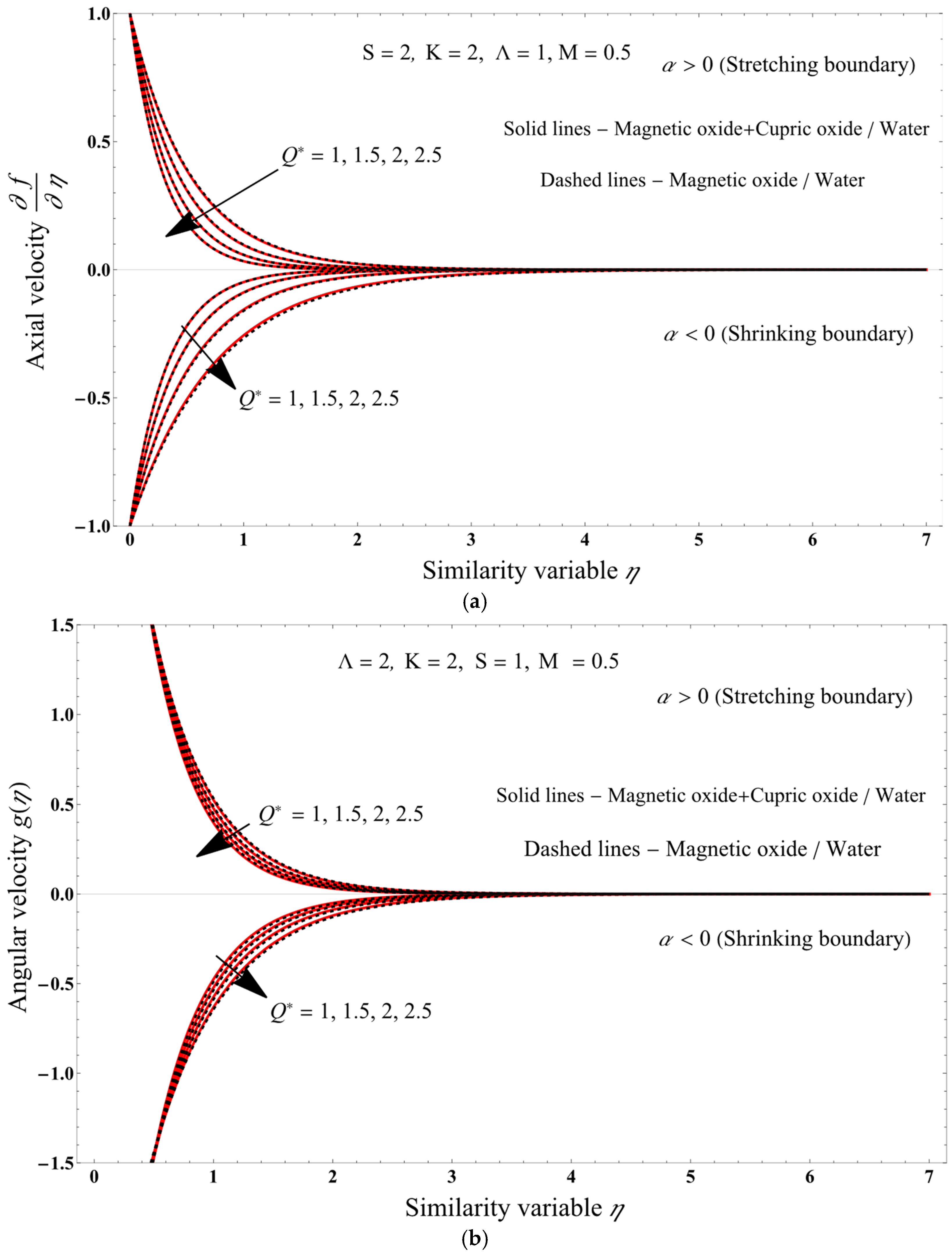
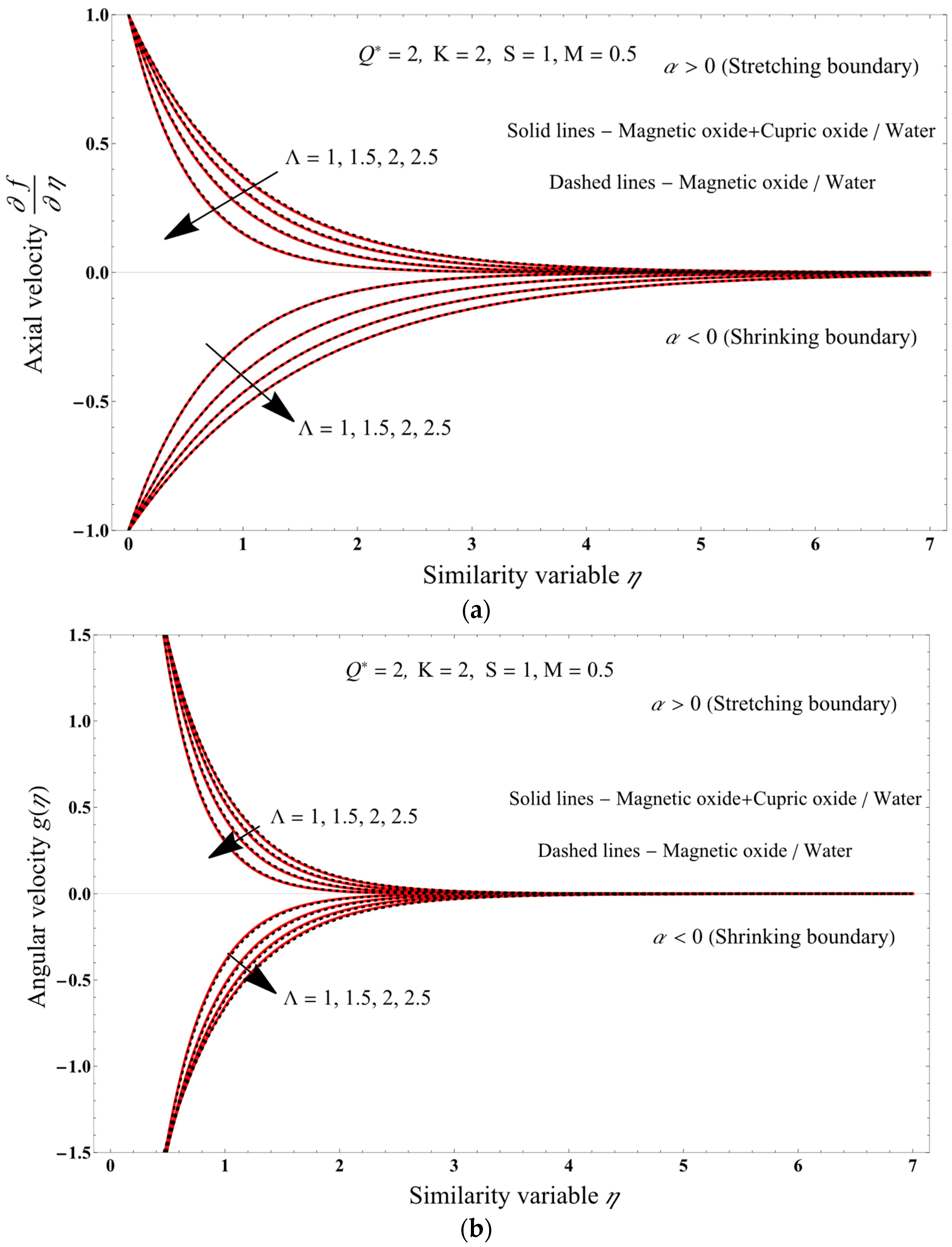
• Increasing the porosity parameter decreases the axial and angular velocities profiles.
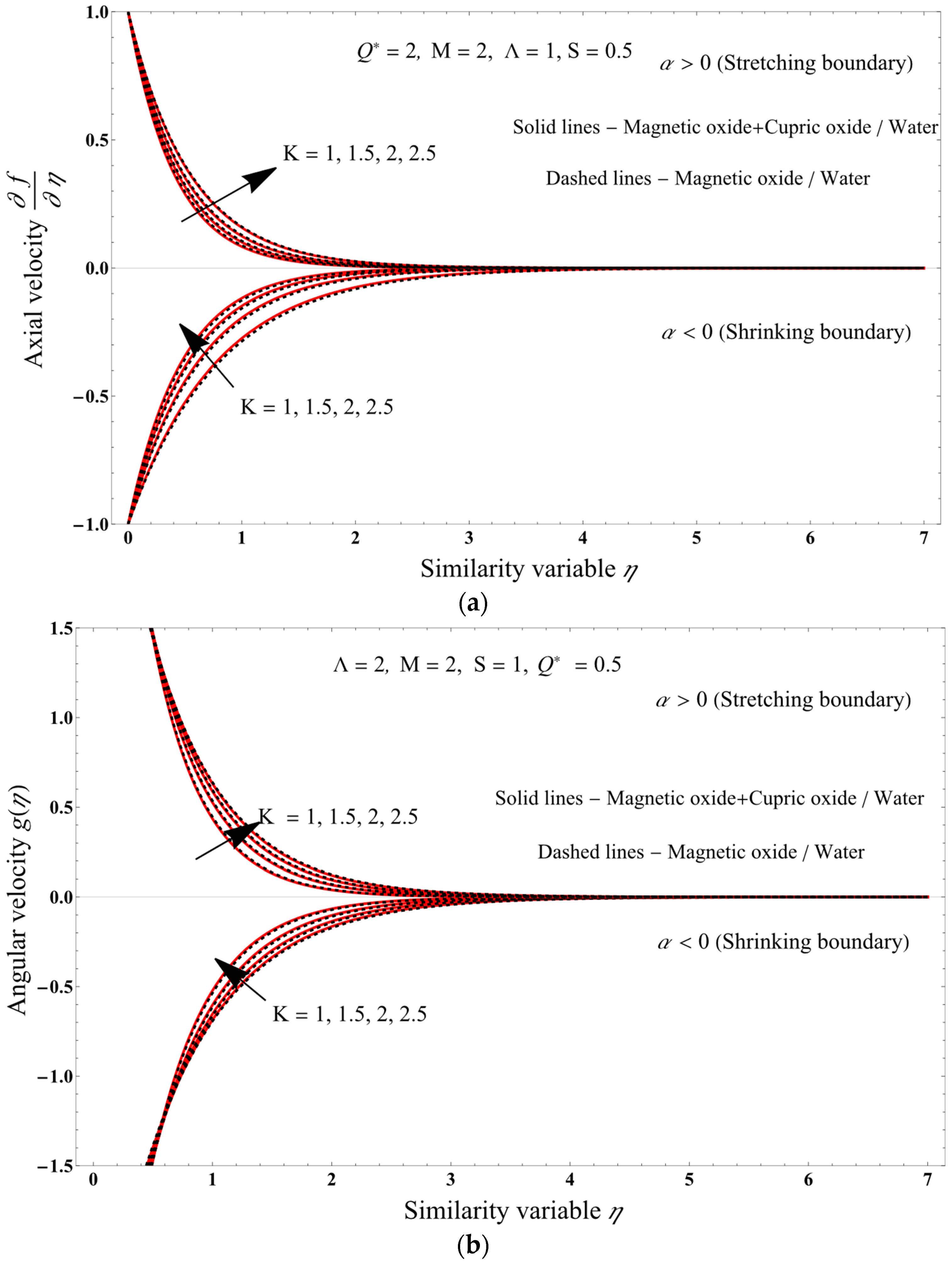
• Increasing the micropolar parameter causes axial and angular velocities increases.
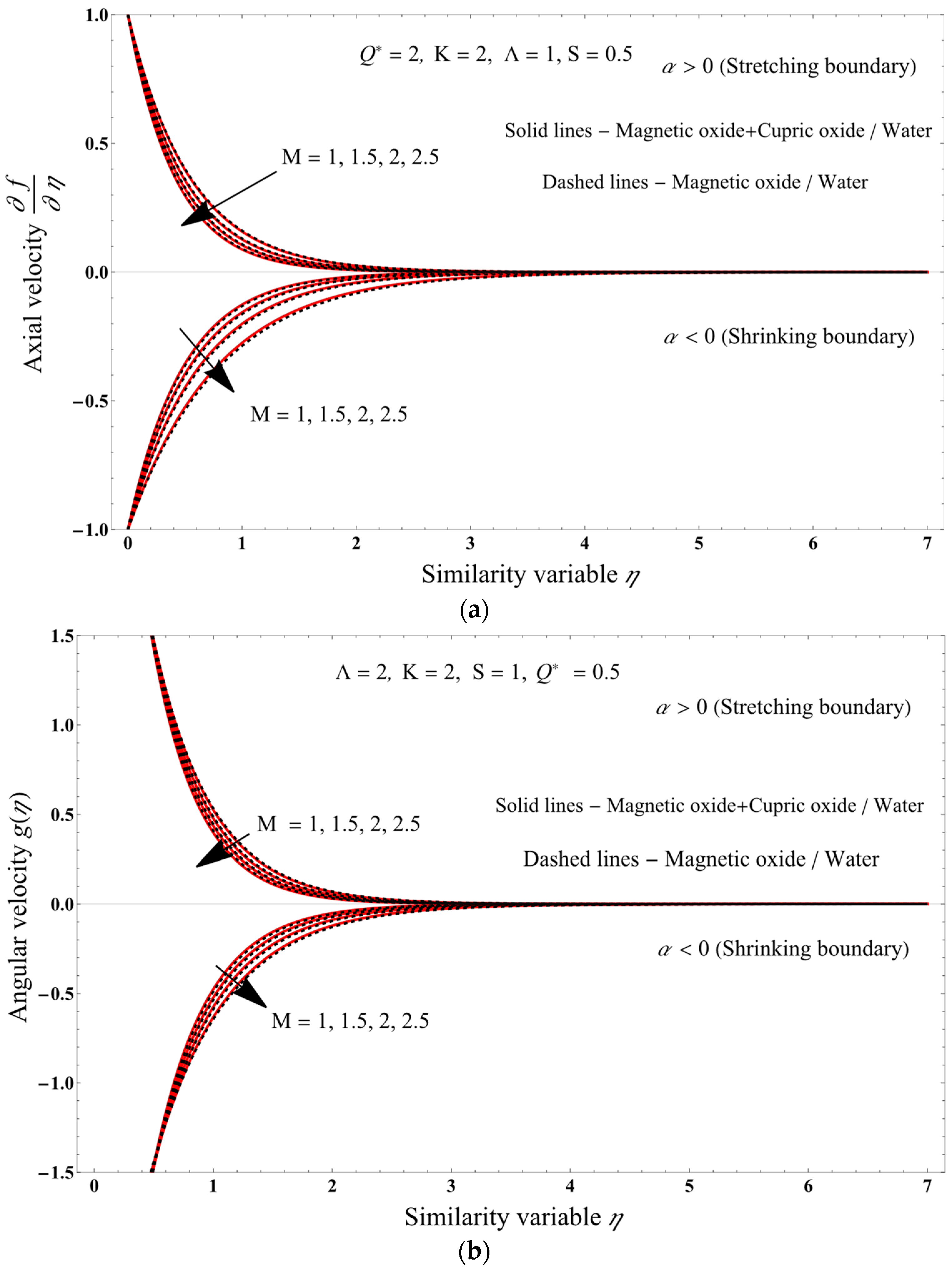
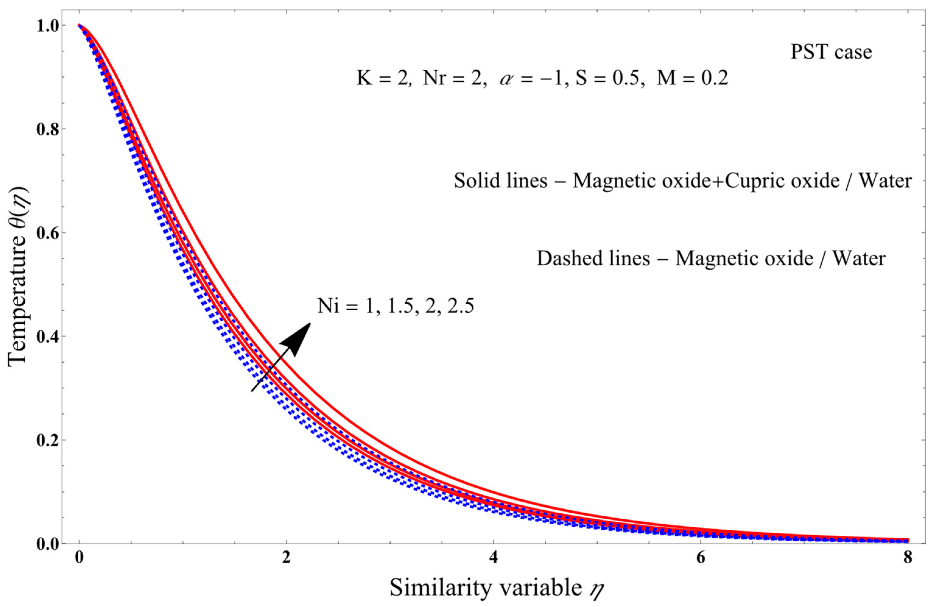
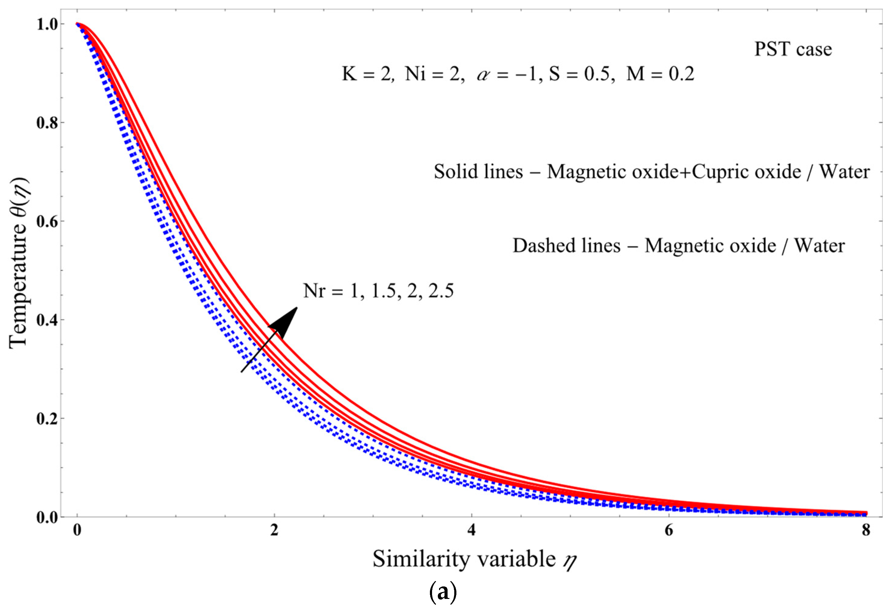
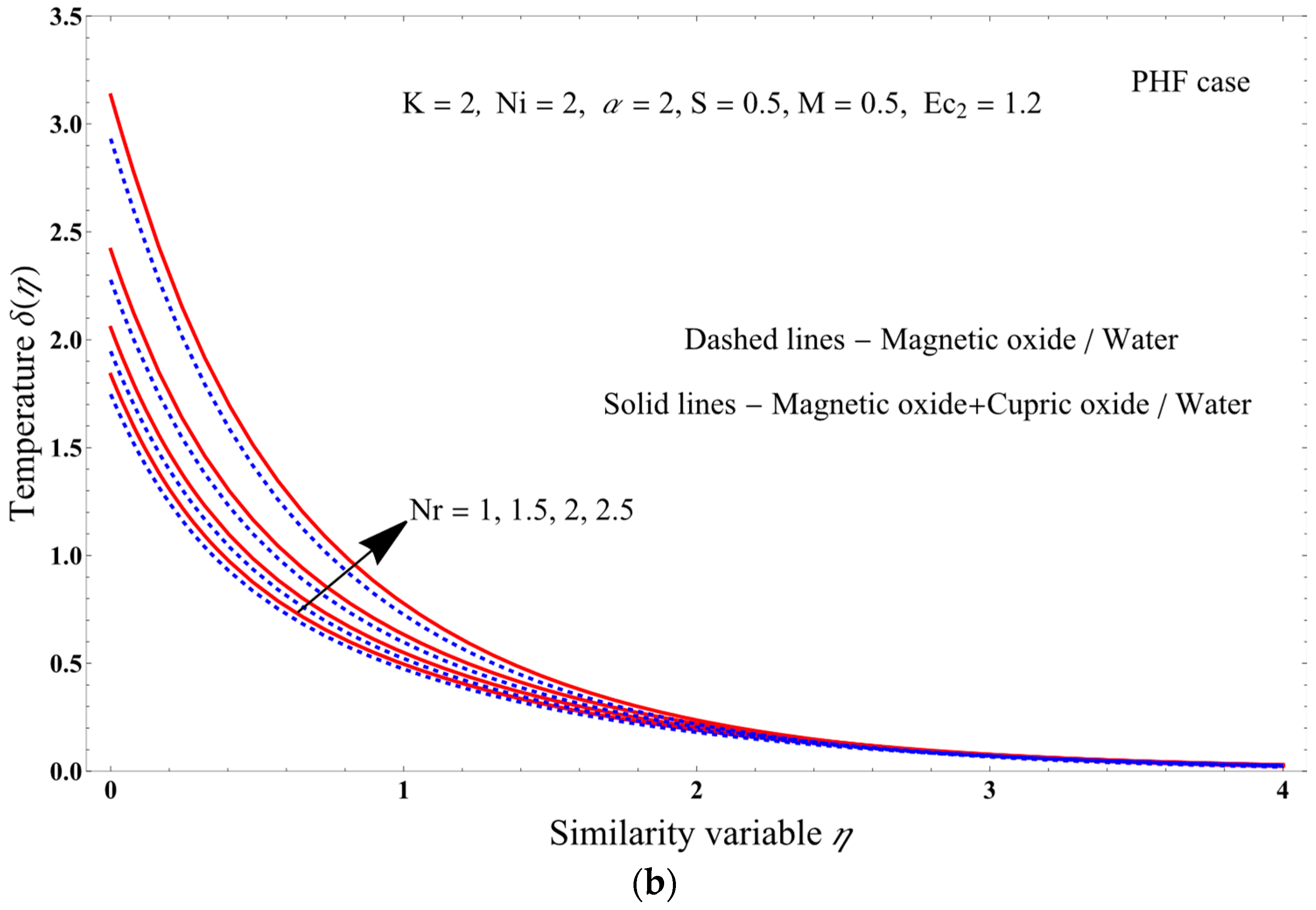
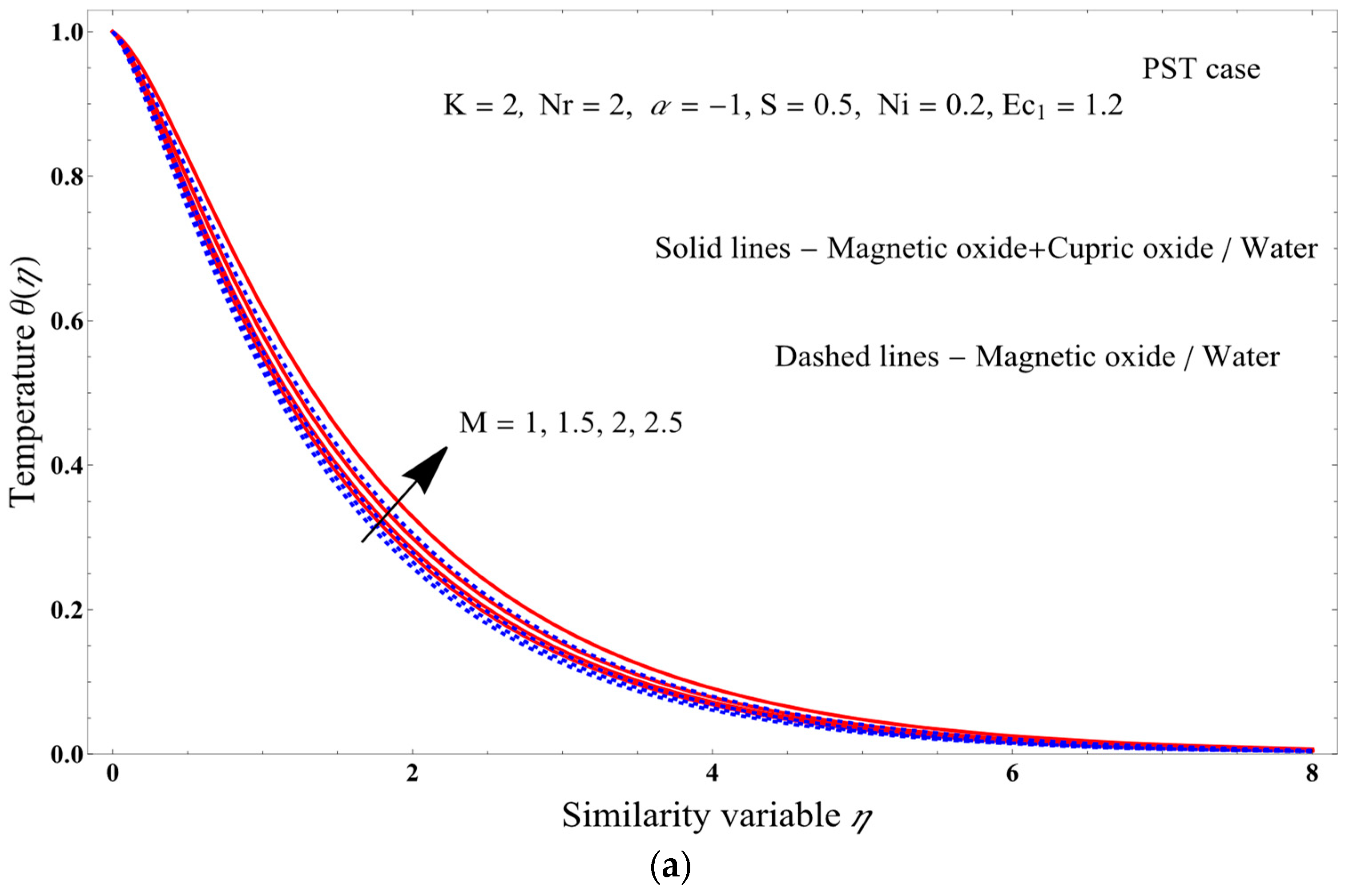
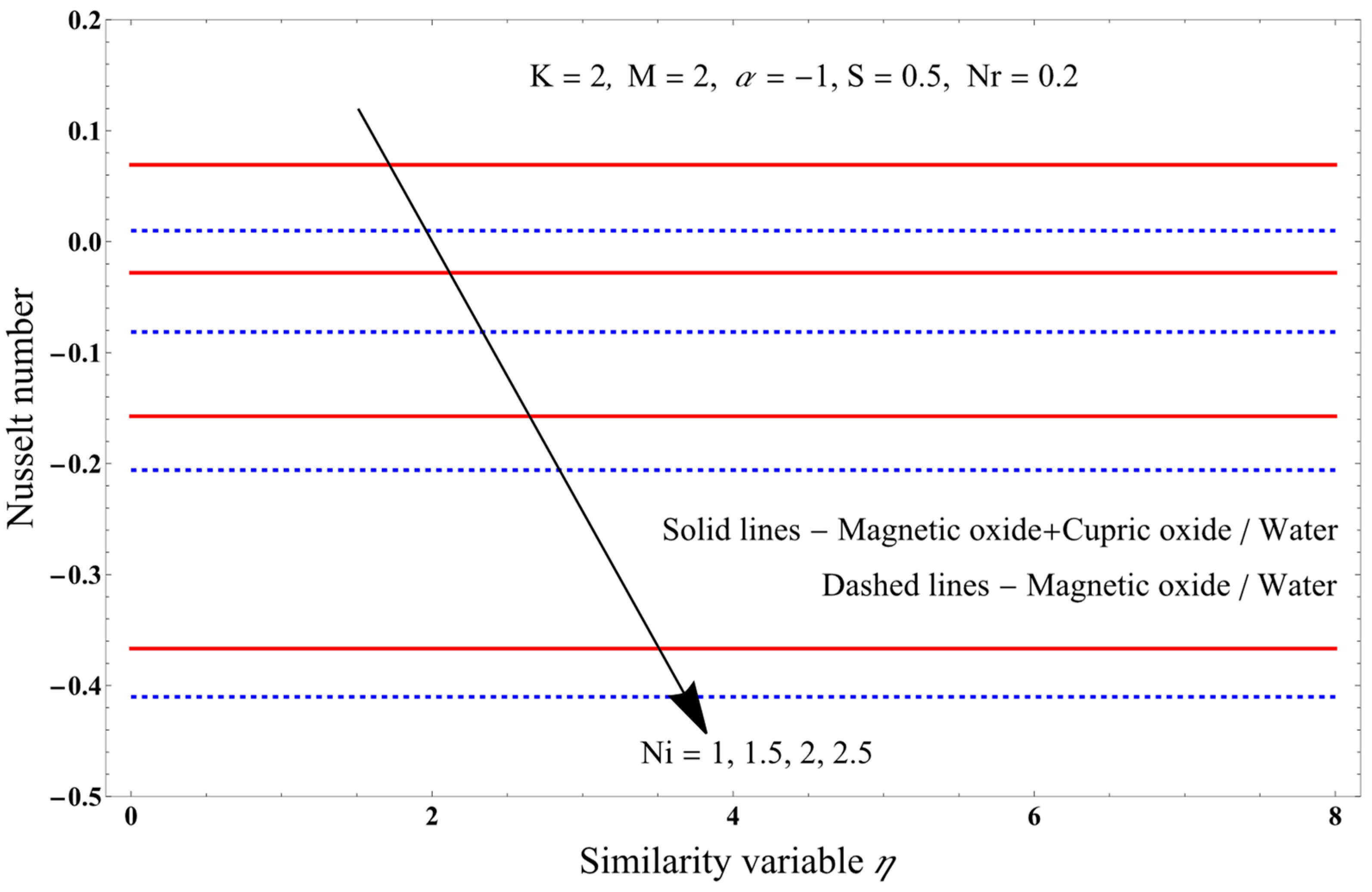
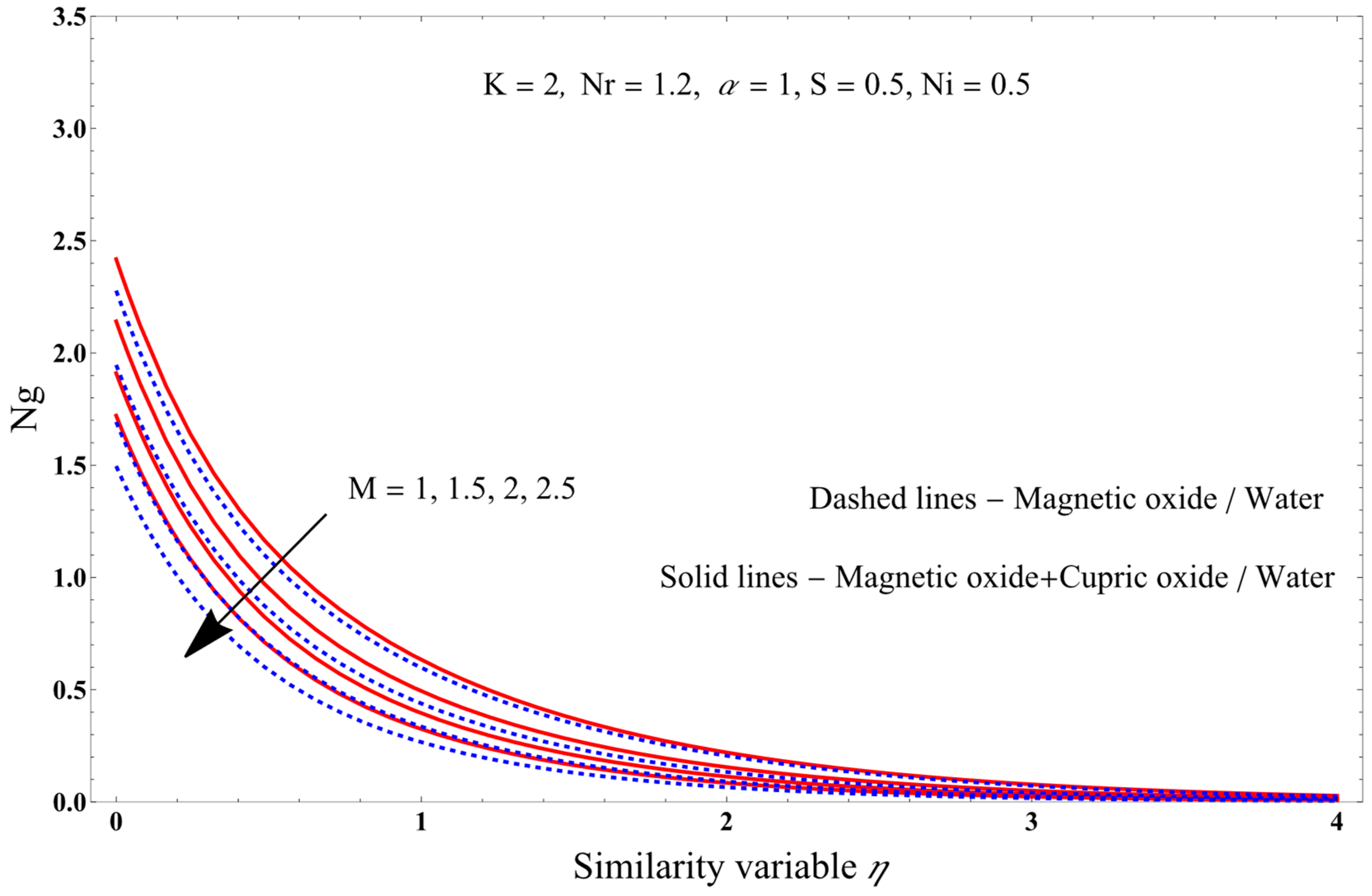
• As the magnetic field increases, axial as well as angular velocities decrease, while the temperature of the PST and PHF cases increases, and the Nusselt number and entropy generation decrease.
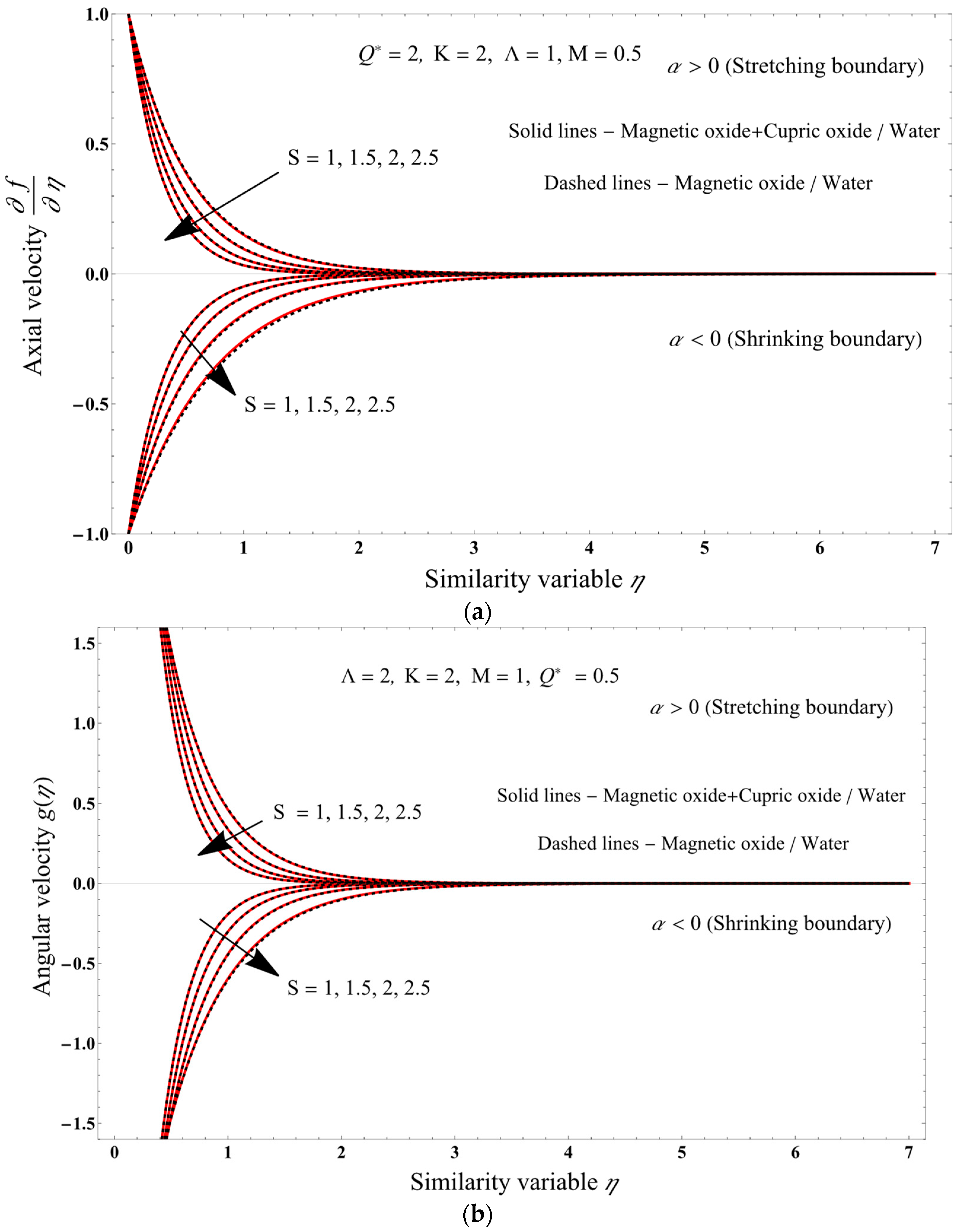
• Increasing the mass transpiration causes axial and angular velocities decrease.
• Increasing the Magnetic field raises the skin friction.
• Increasing the thermal diffusivity increases the skin friction.
• Increasing the Brinkman number decreases the axial and angular velocities.
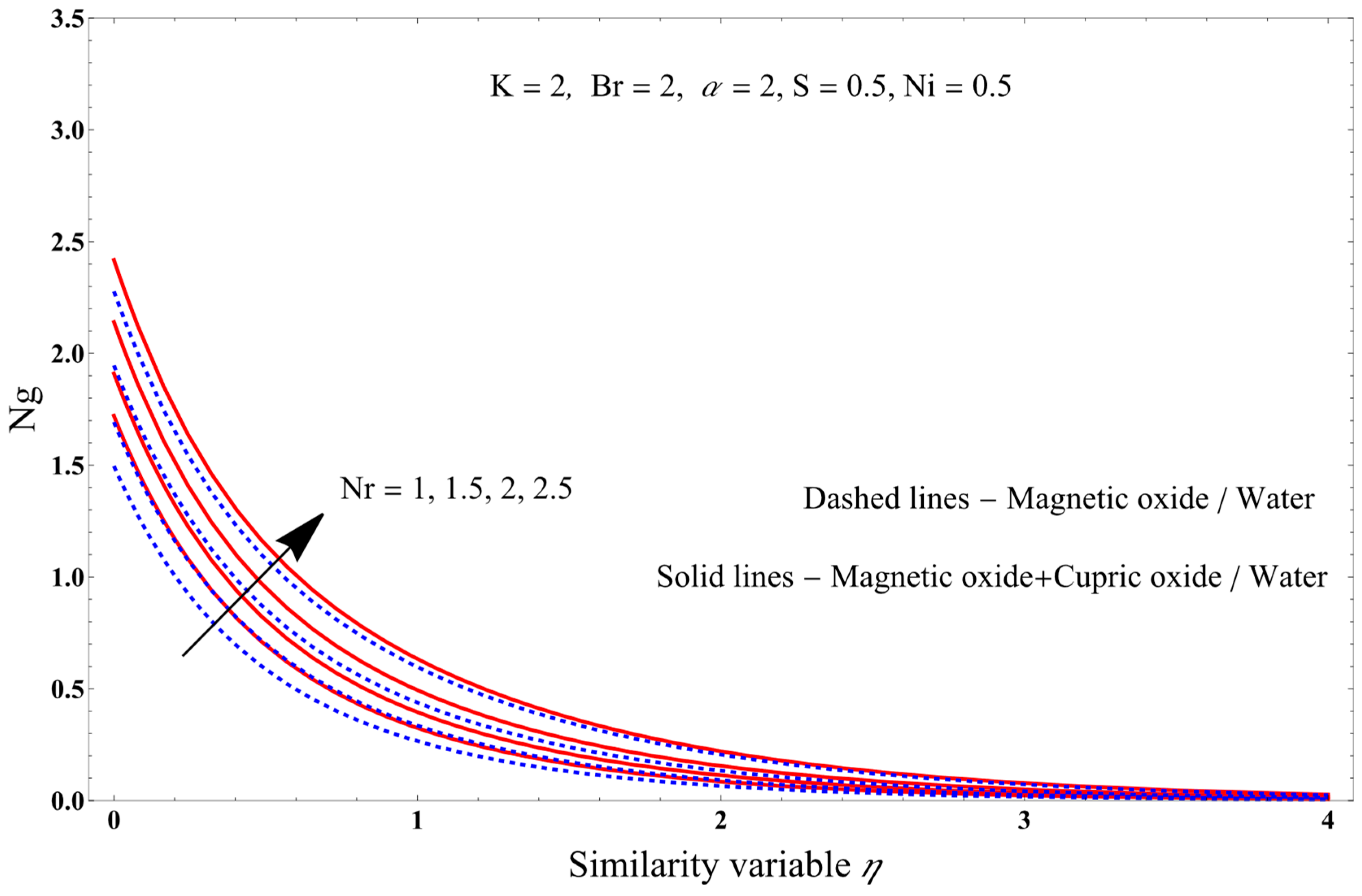
• Increasing the Nr parameter increases the temperature for the PST and PHF cases, and the entropy production.
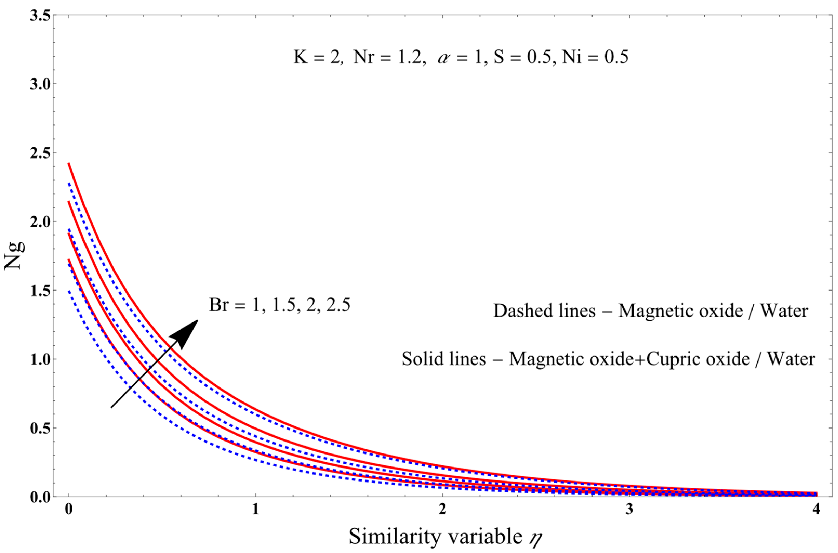
• As the Brickman number increases, the entropy production increases.

The current research sheds new light on the field of fluid dynamics by considering the complex interactions of viscoelastic and Maxwell fluids within porous media. Incorporating couple stress effects further enrich the study, suggesting a more comprehensive understanding of the behaviors under various conditions. The application of these findings to Riga plates as well as convergent divergent channels and exponential stretching sheets opens new horizons to the knowledge in engineering and technology leading to innovative solutions to contemporary challenges in fluid mechanics. Meantime a significant limitation of the hypergeometric series solution method used here is its reliance on convergence criteria, which may not be satisfied in highly nonlinear systems with multiple interacting phenomena.

References

1. Raghunath, K.; Gulle, N.; Vaddemani, R.R.; Mopuri, O. Unsteady MHD fluid flow past an inclined vertical porous plate in the presence of chemical reaction with aligned magnetic field, radiation, and Soret effects. Heat Transf. 2022, 51, 2742–2760. [Google Scholar] [CrossRef]
2. Li, Z.; Li, K.; Guo, X.; Gao, X.; Dai, W.; Gong, M.; Shen, J. Influence of timing between magnetic field and fluid flow in a rotary magnetic refrigerator. Appl. Therm. Engin. 2021, 187, 116477. [Google Scholar] [CrossRef]
3. Zhang, X.; Zhang, Y. Experimental study on enhanced heat transfer and flow performance of magnetic nanofluids under alternating magnetic field. Int. J. Therm. Sci. 2021, 164, 106897. [Google Scholar] [CrossRef]
4. Vinod, Y.; Nagappanavar, S.N.; Raghunatha, K.R.; Sangamesh. Dufour and Soret effects on double diffusive Casson fluid flow with the influence of internal heat source. J. Umm Al-Qura Univ. Appl. Sci. 2024, in print. [CrossRef]
5. Qi, L.; Zhang, Q.; Niu, S.; Chen, R.; Li, Y. Influencing mechanism of an external magnetic field on fluid flow, heat transfer and microstructure in aluminum resistance spot welding. Engin. Appl. Comput. Fluid Mech. 2021, 15, 985–1001. [Google Scholar] [CrossRef]
6. Ige, E.O.; Oyelami, F.H.; Adedipe, E.S.; Tlili, I.; Khan, M.I.; Khan, S.U.; Malik, M.Y.; Xia, W.F. Analytical simulation of nanoparticle-embedded blood flow control with magnetic field influence through spectra homotopy analysis method. Int. J. Mod. Phys. B 2021, 35, 2150226. [Google Scholar] [CrossRef]
7. Teng, B.; Luo, W.; Chen, Z.; Kang, B.; Chen, L.; Wang, T. A comprehensive study of the effect of Brinkman flow on the performance of hydraulically fractured wells. J. Petrol. Sci. Engin. 2022, 213, 110355. [Google Scholar] [CrossRef]
8. Zhang, L.; Bhatti, M.M.; Michaelides, E.E. Electro-magnetohydrodynamic flow and heat transfer of a third-grade fluid using a Darcy–Brinkman–Forchheimer model. Int. J. Numer. Meth. Heat Fluid Flow 2021, 31, 2623–2639. [Google Scholar] [CrossRef]
9. El-Sapa, S. Effect of permeability of Brinkman flow on thermophoresis of a particle in a spherical cavity. Eur. J. Mech. B Fluids 2020, 79, 315–323. [Google Scholar] [CrossRef]
10. Sachhin, S.M.; Mahabaleshwar, U.S.; Laroze, D.; Drikakis, D. Darcy–Brinkman model for ternary dusty nanofluid flow across stretching/shrinking surface with suction/injection. Fluids 2024, 9, 94. [Google Scholar] [CrossRef]
11. Li, H.; Wang, S.; Wang, R.; Liu, Y.; Shao, B.; Yuan, Z.; Chen, Y.; Ma, Y. Simulation on flow behavior of particles and its effect on heat transfer in porous media. J. Petrol. Sci. Engin. 2021, 197, 107974. [Google Scholar] [CrossRef]
12. Wang, C.; Zheng, X.; Zhang, T.; Chen, H.; Mobedi, M. The effect of porosity and number of unit cell on applicability of volume average approach in closed cell porous media. Int. J. Numer. Meth. Heat Fluid Flow 2022, 32, 2778–2798. [Google Scholar] [CrossRef]
13. Feng, Q.; Cha, L.; Dai, C.; Zhao, G.; Wang, S. Effect of particle size and concentration on the migration behavior in porous media by coupling computational fluid dynamics and discrete element method. Powder Technol. 2020, 360, 704–714. [Google Scholar] [CrossRef]
14. Zhang, J.; Zhang, H.; Lee, D.; Ryu, S.; Kim, S. Study on the effect of pore-scale heterogeneity and flow rate during repetitive two-phase fluid flow in microfluidic porous media. Petrol. Geosci. 2021, 27, 2020–2062. [Google Scholar] [CrossRef]
15. Sachhin, S.M.; Mahabaleshwar, U.S.; Nayakar, S.N.R.; Patil, H.S.R.; Souayeh, B. Darcy–Brinkman model for Boussinesq–Stokes suspension tetra dusty nanofluid flow over stretching/shrinking sheet with suction/injection. Numer. Heat Transf. A Appl. 2024, in print. [CrossRef]
16. Tsiberkin, K. Porosity effect on the linear stability of flow overlying a porous medium. Eur. Phys. J. E 2020, 43, 34. [Google Scholar] [CrossRef] [PubMed]
17. Sachhin, S.M.; Mahabaleshwar, U.S.; Zeidan, D.; Joo, S.W.; Manca, O. An effect of velocity slip and MHD on Hiemenz stagnation flow of ternary nanofluid with heat and mass transfer. J. Therm. Anal. Calorim. 2024, in print. [CrossRef]
18. Sangamesh; Vinod, Y.; Waqas, H.; Raghunatha, K.R.; Nagappanavar, S.N. Mixed convection over an exponentially stretching surface with the effect of radiation and reaction. Nano. 2024, in print. [CrossRef]
19. Li, S.; Raghunath, K.; Alfaleh, A.; Ali, F.; Zaib, A.; Khan, M.I.; Iljaz Khan, M.; Puneeth, V. Effects of activation energy and chemical reaction on unsteady MHD dissipative Darcy–Forchheimer squeezed flow of Casson fluid over horizontal channel. Sci. Rep. 2023, 13, 2666. [Google Scholar] [CrossRef]
20. Zhang, L.; Bhatti, M.M.; Shahid, A.; Ellahi, R.; Bég, O.A.; Sait, S.M. Nonlinear nanofluid fluid flow under the consequences of Lorentz forces and Arrhenius kinetics through a permeable surface: A robust spectral approach. J. Taiwan Inst. Chem. Engin. 2021, 124, 98–105. [Google Scholar] [CrossRef]
21. Ibrahim, W.; Negera, M. MHD slip flow of upper-convected Maxwell nanofluid over a stretching sheet with chemical reaction. J. Egypt. Math. Soc. 2020, 28, 7. [Google Scholar] [CrossRef]
22. Xiong, P.Y.; Chu, Y.M.; Khan, M.I.; Khan, S.A.; Abbas, S.Z. Entropy optimized Darcy–Forchheimer flow of Reiner–Philippoff fluid with chemical reaction. Comput. Theor. Chem. 2021, 1200, 113222. [Google Scholar] [CrossRef]
23. Ali, L.; Ali, B.; Liu, X.; Ahmed, S.; Shah, M.A. Analysis of bio-convective MHD Blasius and Sakiadis flow with Cattaneo–Christov heat flux model and chemical reaction. Chin. J. Phys. 2022, 77, 1963–1975. [Google Scholar] [CrossRef]
24. Roy, A.K.; Bég, O.A. Mathematical modelling of unsteady solute dispersion in two-fluid (micropolar–Newtonian) blood flow with bulk reaction. Int. Commun. Heat Mass Transf. 2021, 122, 105169. [Google Scholar] [CrossRef]
25. Kocić, M.; Stamenković, Ž.; Petrović, J.; Bogdanović–Jovanović, J. MHD micropolar fluid flow in porous media. Adv. Mech. Engin. 2023, 15, 16878132231178436. [Google Scholar] [CrossRef]
26. Ali, L.; Liu, X.; Ali, B.; Mujeed, S.; Abdal, S.; Mutahir, A. The impact of nanoparticles due to applied magnetic dipole in micropolar fluid flow using the finite element method. Symmetry 2020, 12, 520. [Google Scholar] [CrossRef]
27. Deo, S.; Maurya, D.K.; Filippov, A.N. Effect of magnetic field on hydrodynamic permeability of biporous membrane relative to micropolar liquid flow. Colloid J. 2021, 83, 662–675. [Google Scholar] [CrossRef]
28. Raghunatha, K.R.; Vinod, Y.; Nagappanavar, S.N.; Sangamesh. Unsteady Casson fluid flow on MHD with an internal heat source. J. Taibah Univ. Sci. 2023, 17, 2271691. [Google Scholar] [CrossRef]
29. Maurya, D.K.; Deo, S.; Khanukaeva, D.Y. Analysis of Stokes flow of micropolar fluid through a porous cylinder. Math. Meth. Appl. Sci. 2021, 44, 6647–6665. [Google Scholar] [CrossRef]
30. Vajravelu, K.; Hadjinicolaou, A. Heat transfer in a viscous fluid over a stretching sheet with viscous dissipation and internal heat generation. Int. Commun. Heat Mass Transf. 1993, 20, 417–430. [Google Scholar] [CrossRef]
31. Sachhin, S.M.; Mahabaleshwar, U.S.; Chan, A. Effect of slip and thermal gradient on micropolar nano suspension flow across a moving hydrogen fuel-cell membrane. Int. J. Hydrogen Energy 2024, 63, 59–81. [Google Scholar] [CrossRef]
32. Gireesha, B.J.; Mahanthesh, B.; Gorla, R.S.R. Suspended particle effect on nanofluid boundary layer flow past a stretching surface. J. Nanofl. 2014, 3, 267–277. [Google Scholar] [CrossRef]
33. Singh, P.K.; Anoop, K.B.; Sundararajan, T.; Das, S.K. Entropy generation due to flow and heat transfer in nanofluids. Int. J. Heat Mass Transf. 2010, 53, 4757–4767. [Google Scholar] [CrossRef]
34. Srinivasacharya, D.; Hima Bindu, K. Entropy generation in a micropolar fluid flow through an inclined channel. Alexandr. Engin. J. 2016, 55, 973–982. [Google Scholar] [CrossRef]
35. Avramenko, A.A.; Tyrinov, A.I.; Shevchuk, I.V.; Dmitrenko, N.P. Dean instability of nanofluids with radial temperature and concentration non-uniformity. Phys. Fluids 2016, 28, 034104. [Google Scholar] [CrossRef]
36. Avramenko, A.A.; Shevchuk, I.V.; Abdallah, S.; Blinov, D.G.; Harmand, S.; Tyrinov, A.I. Symmetry analysis for film boiling of nanofluids on a vertical plate using a nonlinear approach. J. Mol. Liq. 2016, 223, 156–164. [Google Scholar] [CrossRef]
37. Sajid, M.; Ahmad, I.; Hayat, T.; Ayub, M. Unsteady flow and heat transfer of a second-grade fluid over a stretching sheet. Commun. Nonlinear Sci. Numer. Simul. 2009, 14, 96–108. [Google Scholar] [CrossRef]
38. Ishak, A.; Nazar, R.; Pop, I. Heat transfer over a stretching surface with variable heat flux in micropolar fluids. Phys. Lett. A 2008, 372, 559–561. [Google Scholar] [CrossRef]
39. Ishak, A.; Nazar, R.; Pop, I. Mixed convection boundary layers in the stagnation-point flow toward a stretching vertical sheet. Meccanica 2006, 41, 509–518. [Google Scholar] [CrossRef]
40. Nazar, R.; Amin, N.; Filip, D.; Pop, I. Stagnation point flow of a micropolar fluid towards a stretching sheet. Int. J. Non-Linear Mech. 2004, 39, 1227–1235. [Google Scholar] [CrossRef]
41. Crane, L.J. Flow past a stretching plate. Math. Phys. 1970, 21, 645–647. [Google Scholar] [CrossRef]
42. Pavlov, K.B. Magnetohydrodynamic flow of incompressible viscous fluid caused by of a surface. Magnetohydrodyn. 1974, 10, 507–510. Available online: http://www.mhd.sal.lv/contents/1974/4/MG.10.4.23.R.html (accessed on 10 November 2024).
43. Khan, U.; Zaib, A.; Ishak, A.; Roy, N.C.; Bakar, S.A.; Muhammad, T.; Aty, A.H.A.; Yahia, I.S. Exact solutions for MHD axisymmetric hybrid nanofluid flow and heat transfer over a permeable non-linear radially shrinking/stretching surface with mutual impacts of thermal radiation. Eur. Phys. J. Spec. Top. 2022, 231, 1195–1204. [Google Scholar] [CrossRef]
44. Haq, R.U.; Raza, A.; Algehyne, E.A.; Tlili, I. Dual nature study of convective heat transfer of nanofluid flow over a shrinking surface in a porous medium. Int. Commun. Heat Mass Transf. 2020, 114, 104583. [Google Scholar] [CrossRef]
45. Elsaid, E.M.; Abdel-Wahed, M.S. MHD mixed convection Ferro Fe3O4/Cu-hybrid-nanofluid runs in a vertical channel. Chin. J. Phys. 2022, 76, 269–282. [Google Scholar] [CrossRef]
46. Zaib, A.; Khan, U.; Shah, Z.; Kumam, P.; Thounthong, P. Optimization of entropy generation in flow of micropolar mixed convective magnetite (Fe3O4) ferroparticle over a vertical plate. Alexandr. Engin. J. 2019, 58, 1461–1470. [Google Scholar] [CrossRef]
Figure 1. Diagrammatic representation of fluid flow. The red solid circles indicate magnetic oxide (Fe3O4) nanoparticles, the blue solid circles indicate the cupric oxide (CuO) nanoparticles, and the black solid ellipses indicate porous media. The triangular areas show the boundary regions, and the arrows in those show the axis. u is the flow velocity and b is constant.
Physics 06 00082 g001
Figure 2. Axial (a) and angular (b) velocities for various values of the porosity parameter Q*. See text for details.
Physics 06 00082 g002
Figure 3. Axial (a) angular (b) velocities for different values of the micropolar parameter, K.
Physics 06 00082 g003
Figure 4. Axial (a) and angular (b) velocities for various values of the magnetic field parameter M.
Physics 06 00082 g004
Figure 5. Axial (a) and angular (b) velocities for different values of the mass transpiration parameter S.
Physics 06 00082 g005
Figure 6. Axial (a) and angular (b) velocities for different values of the Brinkman number Λ.
Physics 06 00082 g006
Figure 7. Temperature for various values of the Eckert number Ec for the PST (a) and PHF (b) cases. See text for details.
Physics 06 00082 g007
Figure 8. Temperature for different values of the heat source/sink parameter Ni for the PST case.
Physics 06 00082 g008
Figure 9. Temperature for different values of the radiation parameter Nr for the PST (a) PHF (b) cases.
Physics 06 00082 g009aPhysics 06 00082 g009b
Figure 10. Temperature for different values of the magnetic field parameter M for PST (a) and PHF (b) cases and (c) concentration for different values of the Schmidt number Sc.
Physics 06 00082 g010aPhysics 06 00082 g010b
Figure 11. Nusselt number for different values of the heat source/sink parameter Ni.
Physics 06 00082 g011
Figure 12. Nusselt number for different values of the magnetic field parameter M.
Physics 06 00082 g012
Figure 13. Nusselt number for different values of the radiation parameter Nr.
Physics 06 00082 g013
Figure 14. Entropy production for different values of the magnetic field parameter M.
Physics 06 00082 g014
Figure 15. Entropy production for different values of the Brickman number.
Physics 06 00082 g015
Figure 16. Entropy production for different values of the radiation parameter Nr.
Physics 06 00082 g016
Figure 17. Skin friction for different values of the stretching/shrinking parameter α.
Physics 06 00082 g017
Figure 18. Skin friction for different values of the magnetic field parameter M.
Physics 06 00082 g018
Figure 19. The streamlined graphs of hybrid nanofluid (red solid lines) and nanofluid (dashed blue lines) flows for different sets of parameters (af) as indicated.
Physics 06 00082 g019aPhysics 06 00082 g019b