Abstract
Ant colony optimization (ACO) is a stochastic optimization algorithm inspired by the foraging behavior of ants. We investigate a simplified computational model of ACO, wherein ants sequentially engage in binary decision-making tasks, leaving pheromone trails contingent upon their choices. The quantity of pheromone left is the number of correct answers. We scrutinize the impact of a salient parameter in the ACO algorithm, specifically, the exponent , which governs the pheromone levels in the stochastic choice function. In the absence of pheromone evaporation, the system is accurately modeled as a multivariate nonlinear Pólya urn, undergoing phase transition as varies. The probability of selecting the correct answer for each question asymptotically approaches the stable fixed point of the nonlinear Pólya urn. The system exhibits dual stable fixed points for and a singular stable fixed point for where is the critical value. When pheromone evaporates over a time scale , the phase transition does not occur and leads to a bimodal stationary distribution of probabilities for and a monomodal distribution for .
1. Introduction
Sociophysics emerged in the 1970s and has evolved into a captivating research field within statistical physics [1,2]. In particular, herding behavior, or the inclination to follow the majority, has captured the attention of many researchers due to its pivotal role in understanding social phenomena [3,4,5,6,7]. Various probabilistic models have been proposed to describe herding behavior, with one notable example being the ant recruitment model [8,9]. This model explains the intermittent oscillation observed in ants when they are presented with two identical food sources [10,11]. When ants choose a food source from among two food sources, the ant recruitment model incorporates a straightforward herding mechanism in which a randomly selected ant chooses one of the two based on the number of ants that have already made the same choice. Scouts play a crucial role by exploring the terrain to locate food sources [12,13]. When a scout discovers food, it returns to the nest, leaving a pheromone trail in its wake. Other ants are drawn to these pheromone marks and consequently become recruited to forage at the food source.
Ant colony optimization (ACO) is a model-based meta-heuristic inspired by the foraging behavior of ants in their search for the shortest path to food sources [14,15,16,17,18]. While ants may not be highly intelligent individually, they collectively find the shortest path by following pheromone trails left by their fellow ants. The optimal path is determined by the route on which the maximum number of ants travel. Consider a classic problem known as the traveling salesman problem (TSP), which involves finding the shortest possible route that visits each city represented as vertices in a given graph exactly once and returning to the origin city [19]. In ACO, ants make decisions about their next city to visit based on a concept called “pheromone”. Pheromone represents the preference for a particular choice and is collaboratively learned by the ants during their search process [15]. In the context of the TSP defined on a graph, pheromone values are typically associated with edges between cities, reflecting the preference for traveling from one city to another along the corresponding edges. These pheromone values are learned through a reinforcement strategy, where each ant reinforces its chosen paths based on the quality of the solution constructed. This quality is often determined using the inverse of the total length of the route. ACO has found successful applications in various industrial and academic constraint optimization problems and has become one of the most popular methods [20,21,22,23].
ACO has seen significant improvements, and modern ACO algorithms deviate substantially from the original ACO [24]. The fundamental modification lies in controlling the diversity of solutions and achieving convergence [25,26]. In this context, “convergence” refers to the tendency of ants to cluster around similar solutions in the neighborhood and ultimately converge toward the same solution. Early convergence to a small region of the search space leaves large enough sections of the search space unexplored and fails to find suitable solutions. On the other hand, quite slow convergence means that the computational cost required to reach acceptable solutions is high, rendering the search inefficient. Diversity control aims to prevent complete convergence by slowing down the search process.
Many algorithms have been proposed for controlling the diversity of the ACO algorithm. One of the diversity control mechanisms involves modifying the probabilistic decision function [24,27]. Bernd Meyer studied the influence of , the exponent on the pheromone level in the selection function, and suggested that qualitatively determines diversity and convergence behavior. Additionally, Meyer introduced a dynamic that changes throughout the search process to enhance search efficiency, a technique known as -“annealing”. Meyer also emphasized the significance of noise in ACO using stochastic differential equations in both static and dynamic environments [24,28,29,30]. Ants respond to a two-choice question, and the noisy communication among ants prevents them from selecting suboptimal choice. In this paper, we study a simple model of ACO in which ants sequentially answer a series of two-choice quizzes. We investigate the phase transition and the qualitative change of the convergence behavior by varying . We start from the discrete time formulation of the problem. Our approach can be straightforwardly generalized to ACO for many-body problems, allowing us to derive the model parameters of the continuous time approach concretely. Additionally, there are various possibilities for the continuous time limit, apart from Wiener noise [31]. In Section 2, we introduce a model and derive stochastic differential equations (SDEs) using diffusion approximation. In Section 3, we investigate the time evolution and examine the effect of on the convergence properties of the solutions. Section 4 provides a summary of the results. Appendix A explains the estimation of the initial conditions for the SDEs.
2. Method and Definitions
There are N two-choice questions, each of which is answered by quite a large number of ants sequentially [32]. These questions are labeled by . The answer provided by the tth ant is denoted as , where indicates a correct answer, and indicates an incorrect answer. In ACO, multiple ants typically search for the optimal solution simultaneously in each iteration. However, in our model, only one ant conducts the search. Each ant receives 1 point for a correct answer. After ant t has answered all N questions, the total points (TPs) earned by the ant can be calculated using the following equation:
Ant t deposits pheromones on their answer . The amount of the pheromones is . We assume that the pheromones evaporate and decrease by per unit time, where represents the time scale of the pheromone evaporation.
Ant observes the total values of the pheromones associated with question m for each choice . We denote the total value of pheromones that remains on all the questions after ant t has answered,
Then, the remaining pheromone on is
The remaining pheromone on is given by .
Ants are not highly intelligent, and the probability of them making the correct choice in the two-choice questions by themselves is 1/2. The information provided by TPs gives them an indirect clue about the correct choice. If TP, the posterior probability for is larger than . Similarly, if is greater than , the posterior probability for is greater than . In ACO, a decision function with a positive parameters and K is introduced that uses the values of the pheromones as follows:
Here, the exponent determines the response of the choice to the values of the pheromones. As K is positive, one can avoid and becoming the absorbing states of the process. However, instead of K, we adopt the following form for the choice function:
Here, is a small positive constant to avoid the absorbing states and of the stochastic process [8].
We denote the ratio of the remaining pheromones on the correct choices as ,
We divide both the denominator and numerator of Equation (3) by , and the probability of the correct choice is expressed as
Here, is defined as
We note that and . The slope of at is . We also introduce the discount factor and the ratio of correct answers as
Stochastic Differential Equations
First, let us derive the recursive relation for and . According to the definition, and obey the next recursive relations
If is finite, for , we have . In the limit , the pheromone does not evaporate, and one has .
For , we can replace the sum of , by the sum of the expected values using the law of large numbers; then:
Let us denote the average of as
Then,
The recursive relation for is
is given as
In the continuous time limit , one obtains:
One sees that converges to . When the pheromones evaporate and , , and the prefactor of the differential equation is . If one assumes that the dynamics of are faster than those of (adiabatic approximation), the time scale of the convergence is given by as . When the pheromone does not evaporate and , . The prefactor of the differential equation is , and . The convergence becomes quite slow.
Next, let us study the dynamics of . The recursive relation for is
is then estimated as
Using , one obtains:
We denote the history of , , as , and the conditional expected value of is estimated as
Likewise, the conditional variance of can be approximated as
Here, we neglect the subleading terms in . We read the drift and diffusion term from the results and the SDEs are
Here, is the Wiener process. Equations (5) and (7) describe the dynamics of the system. The system can be described as a multivariate Pólya urn process.
We note that in Equation (6) breaks the symmetry of the system. If one neglects the term, is proportional to . As , holds. and obey the same dynamics, and we call the symmetry symmetry. The term is always positive and drives in the positive direction. As the term is proportional to , the strength of the -symmetry-breaking field becomes smaller as N becomes larger.
3. Results
We analyze the SDEs given in Equation (7) and investigate the convergence properties of . As the convergence behavior relies on the initial value of in the context of the nonlinear Pólya urn model, we commence by examining the initial distribution of .
3.1. Initial Distribution of
We assume that ants adopt and do not respond to the values of the pheromones for . The ants answer the questions independently, and . We estimate and for as follows:
where N denotes the normal distribution with the mean a and the variance b. The details of the calculations are given in Appendix A. If is finite, one has for . In the limit , the pheromone does not evaporate and then .
The essential differences between and include a shift in the expected value by and the presence of a factor of N in the numerator of the variance of . The shift of arises from the finding that in is 1, which is larger than for . The value of the pheromone contains information about the correct choice, leading to . However, in the “cheating” process, the variables , are combined by , as in Equation (2), resulting in a larger variance for . The factor of N in the numerator of the variance of is a consequence of this combination process.
From the distribution of , one can determine the values of or that guarantee that is greater than 0.5 for the limits and , respectively. With a confidence level of 1%, and should satisfy the following conditions:
3.2. Case with
We take the limit in Equations (5) and (7). We replace and with and , respectively. This results in the following equations:
The initial conditions of and at are as follows:
In the adiabatic approximation, where the time development of is much faster than that of , the structure of the SDE for each , where , is the same as that of a nonlinear P’olya urn [33,34]. The probability for to converge to a stable solution of the following equation is positive [35],
Here, a stable (unstable) solution of Equation (9) means that the curve of the left-hand-side of the equation crosses the diagonal curve in in the downward (upward) direction [35]. We denote the stable and unstable solutions as and , respectively.
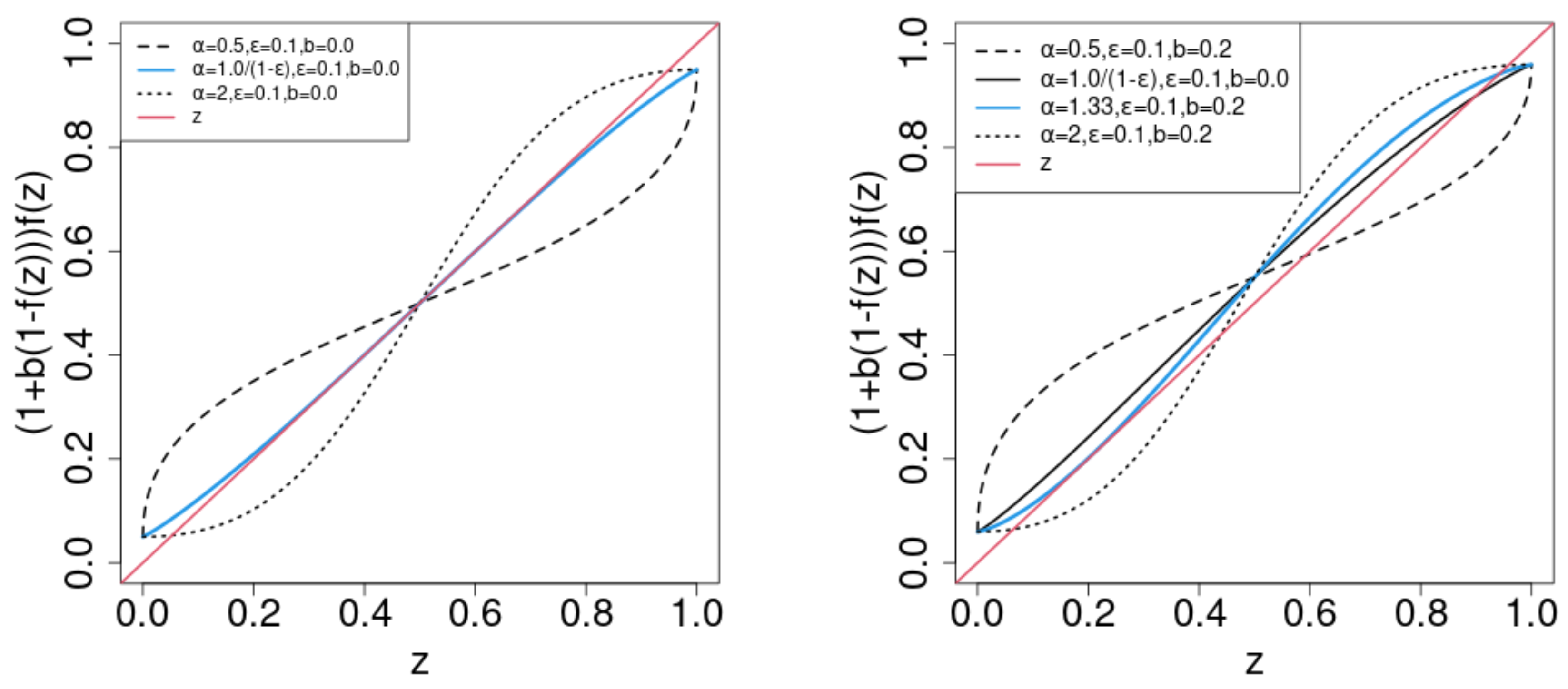
In the limit , the positive driving force in Equation (9) disappears. The system becomes -symmetric, and is a the solution of . If N is finite, the positive driving force breaks the symmetry. We plot in Figure 1. corresponds to and ] for and ; and are used in Figure 1, left and right, respectively, along with .
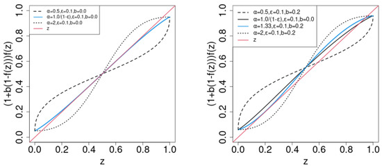
Figure 1.
(4) (left) and (right) versus z for b, , and , as indicated. To visualize the fixed point of , the z-function is also shown.
In the -symmetric case (), the stability of the solution depends on the slope of at . As , where the prime denotes z-derivative, the critical value of is . If , is (un)stable. If , the curve of is tangential to the diagonal. converges to for , as is the unique stable solution . For , there appears two stable solutions : is within , and is within . becomes the unstable solution .
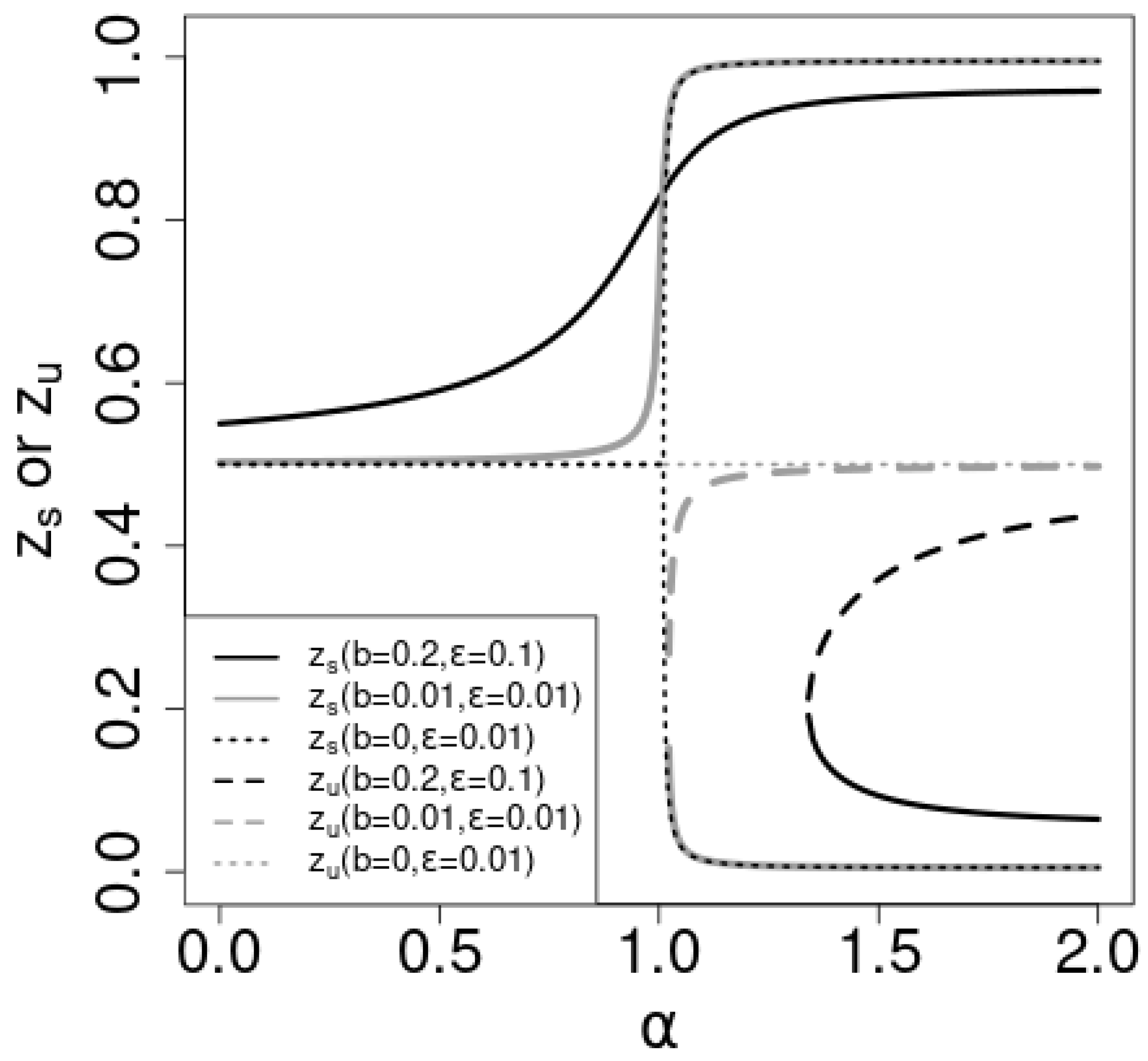
The dotted lines in Figure 2 show the solutions versus for the -symmetric case. For , (black dotted line) is the stable solution. For , (gray dotted line) becomes unstable () and two stable solutions depart from continuously with . The stable solution to which converges depends on the initial value of . In general, if is greater (smaller) than , the probability of the convergence to 1 is greater (smaller) than . determines the “attractive domains” for the stable solutions . The susceptibility of the expected value of to the initial value is the order parameter of the nonlinear Pólya urn [33,34]. As the order parameter is proportional to the difference in the two stable states , the order parameter is a continuous function of , and the phase transition is continuous.

Figure 2.
The stable, , and unstable, , solutions for b and parameters, as indicated. See text for details.
In the -asymmetric case (), for , there is a stable solution, , in the z-range . increases with ; at some critical value, , of , the curve becomes tangential to the diagonal at some . is known as a touchpoint and to be stable [36]. As continues to increase beyond , two significant changes occur: a new stable solution, , emerges from the touchpoint , while an unstable solution, , also becomes apparent.
When , only one stable solution, , exists within the range . Conversely, for , the specific stable solution to which converges depends on the initial values of . At , both the stable fixed point and the touchpoint remain stable. The solution to which converges is determined by the initial values of in this case as well. For , the situation mirrors that of . Once , the order parameter becomes positive, and the phase transition becomes discontinuous.
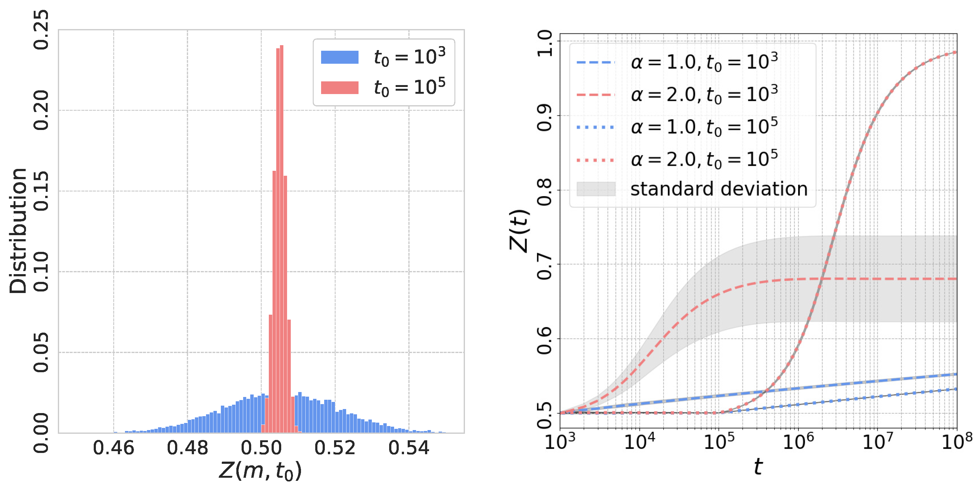
Figure 3 shows the results of the numerical studies in the limit . We sampled a trajectory of and for with and . Figure 3 presents the distribution of for two different values of , namely, . The mean value of is approximately , which aligns with the theoretical predictions. The variance of is given by , so the variance for is about times larger than that for . Consequently, if is chosen, a significant proportion of has , resulting in a high probability that converges to for . In such cases, cannot reach 1 due to the convergence of to . On the other hand, if is set, the ratio of with is zero, ensuring that always converges to . As a result, monotonically increases toward 1 for . For , where only one stable state, , exists, consistently converges to .
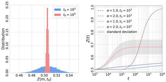
Figure 3.
Left: the initial distribution of for the limit . and are used. Right: versus t for different and as indicated. Gray areas show the standard deviation of which is quite large for and smaller or compatible with the line widths for other cases. See text for details.
One can see that monotonically approaches with time for both and cases within the range . In the case of , where , experiences relatively little change.
3.3. Case with
In the case where is finite, let us make the assumption that and replace with in Equations (5) and (7). This leads to the following equations:
The initial conditions for and at are as follows:
The dynamics of , are coupled through and . To simplify and analyze this coupled system, we focus on the stationary state of in the limit .
are expected to fluctuate around the stable fixed points of in the stationary state. As was observed in Section 3.2 for the case of , for , there is only one stable fixed point, and for , two stable fixed points exist, one of which is near one. The stationary distribution is unimodal for and bimodal for . Let us denote the stationary distribution and the mean value of as and , respectively. As is the probability for , one can assume in the stationary state. The SDEs in Equation (10) can be simplified as follows when replacing and with :
The stationary state with reflecting boundary conditions is determined by a potential solution [37], which can be expressed as:
The second term, , arises from the symmetry-breaking field and causes a shift in the stationary distribution in the positive direction.
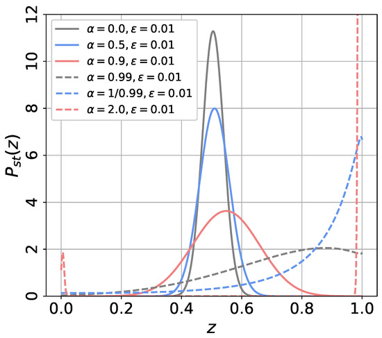
Figure 4.
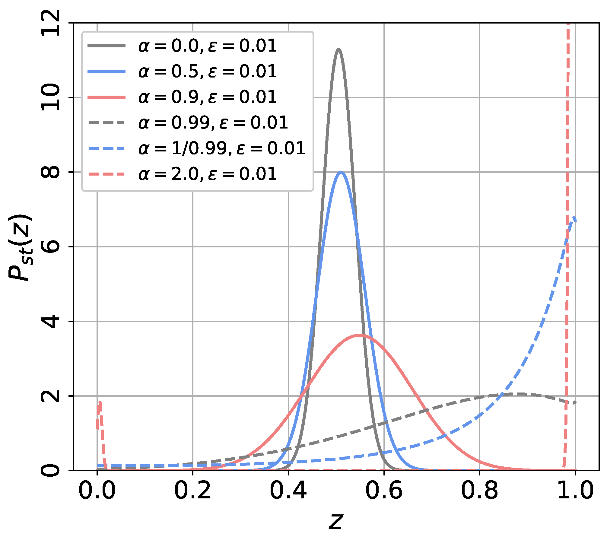
The stationary distribution, (13), for and and parameters as indicated. See text for details.
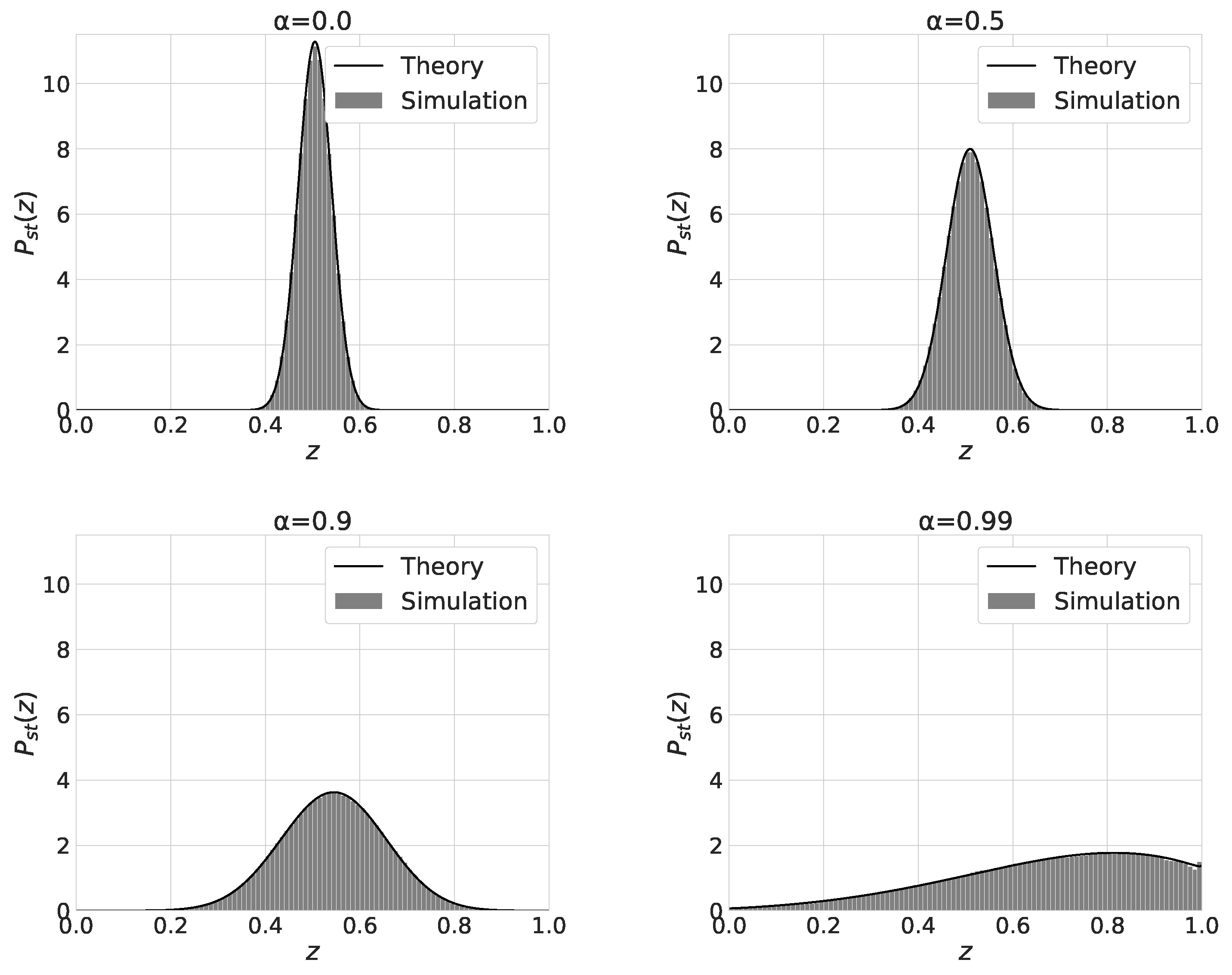
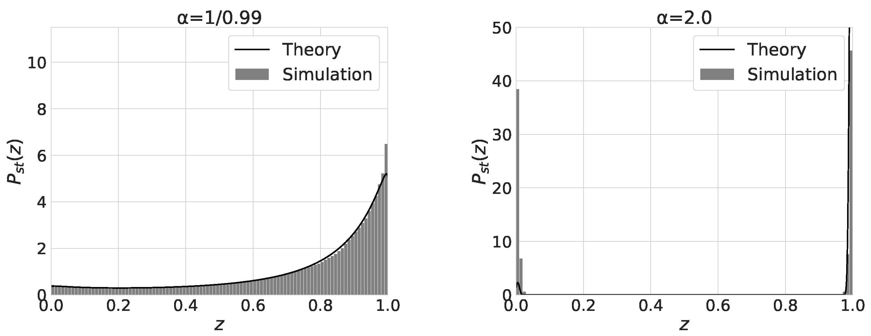
The pair of the parameters are , , , , , and . As increases, the peak position shifts in the positive z-direction, which can be expected by the dependence of the stable solution on in Figure 2. If , the peak appears at , since there is only one stable fixed point near in Figure 1. When , there are two stable fixed point, and the stationary distribution is bimodal.
In order to derive the dependence of and the variance of on , let us assume that fluctuates around for . We linearize in the vicinity of as
Let us also approximate as , then becomes
In the case with , the ants do not observe the information of the pheromones and decide by themselves. The expected value and the variance are consistent with the results (11) for the initial state. The expected value and the variance increase with for .
The shape of the stationary distribution changes from the monomodal shape for to the bimodal shape for . Figure 5 shows the stationary distribution of for and . We also plot in Equation (13) with solid-line curves. Except the case, the numerical results agree with the theoretical ones. As increases from 0 to , the mean value and the variance of increases. For , the distribution of has a peak at . The distribution becomes bimodal and has two peaks near and for . For , becomes bimodal and the equilibration time to reach the stationary state becomes quite long. We beleive the latter is the reason for the discrepancy between the numerical and theoretical results.
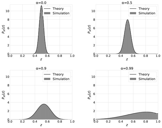
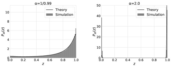
Figure 5.
The distributions of for , and and initial state values as indicated.
4. Discussion
In the presented paper, we studied a simple model for ACO and the convergence properties of the solutions. Ants answer many two-choice questions in sequence and deposit pheromone as they choose. As the amount of the pheromones is the number of correct answers, the following ants can receive information or hints about the correct choices. We showed that the model reduces to a multivariate nonlinear Pólya urn process and the pheromones break the symmetry of the process. By varying the exponent of the decision function of the ants, there occurs a phase transition about the convergence of the probability of choosing the correct answer for each question in the limit . For , the change in the stationary distribution between the monomodal and the bimodal shape occurs as we vary .
Previous studies adopted values of or smaller in solving actual optimization problems, like the TSP [24]. In -annealing, increases gradually, as shown in Ref. [24]. In our study, we showed that the duration of the period should be long enough to ensure that the initial value of is in the attractive domain of the suitable stable state () in the case when . Subsequently, with in effect, converges to a value close to 1. In the case of , the timescale for pheromone evaporation, represented by , shown to be sufficiently long to maintain the same initial conditions. However, does not converge to a specific value; instead, it follows a stationary distribution that exhibits both bimodal and monomodal shapes depending on the value of . To achieve a distribution of with a prominent peak near , the -annealing process is an effective strategy. Both the stable solution and the distribution of suggest that after a lengthy enough period with , it is advantageous to gradually increase from 1. However, the efficiency of the annealing process depends on the specific problem being addressed. Future studies are considered to clarify on an efficient -annealing schedule.
Author Contributions
Conceptualization, S.M. and M.H.; methodology, S.M. and M.H.; software, S.N.; validation, S.M. and S.N.; formal analysis, S.M. and K.N.; investigation, S.N.; resources, S.M.; data curation, S.N.; writing—original draft preparation, S.M.; writing—review and editing, S.M., S.N., K.N. and M.H.; visualization, S.M. and S.N.; supervision, S.M.; project administration, S.M.; funding acquisition, S.M. All authors have read and agreed to the published version of the manuscript.
Funding
This research was funded by JPSJ KAKENHI (grant No. 22K03445), Japan.
Data Availability Statement
We performed numerical simulations using Julia 1.7.3. The code is available at https://github.com/LABO-M/ACO-PhaseTransition-Sampling.git.
Conflicts of Interest
Author Masato Hisakado was employed by the company Nomura Holdings Inc., Tokyo, Japan.
Appendix A. Initial Conditions of Z(t) and Z(m,t)
Let us assume are independent and identically distributed Bernoulli random variable with for and . As soon as and , one finds:
Here, we define as
Applying the central limit theorem, we conclude that behaves like a normal distribution, with its probability density function given by
in Equation (2) is rewritten as
Then, the conditional and unconditional expected values of read
The conditional variance of reads
The unconditional variance reads
We estimate the variance of by neglecting the fluctuation of as
From the central limit theorem, behaves as
References
- Galam, S. Sociophysics: A review of Galam models. Int. J. Mod. Phys. 2008, 19, 409–440. [Google Scholar] [CrossRef]
- Galam, S. Sociophysics: A Physicist’s Modeling of Psycho-Political Phenomena; Springer Science+Business Media, LLC: New York, NY, USA, 2012. [Google Scholar] [CrossRef]
- Galam, S. Majority rule, hierarchical structures, and democratic totalitarianism: A statistical approach. J. Math. Psychol. 1986, 30, 426–434. [Google Scholar] [CrossRef]
- Brian Arthur, W. Competing technologies, increasing returns, and lock-In by historical events. Econ. J. 1989, 99, 116–131. [Google Scholar] [CrossRef]
- Bikhchandani, S.; Hirshleifer, D.; Welch, I. A Theory of fads, fashion, custom, and cultural change as informational cascades. J. Political Econ. 1992, 100, 992–1026. Available online: https://www.jstor.org/stable/2138632 (accessed on 26 December 2023).
- Mori, S.; Hisakado, M.; Takahashi, T. Phase transition to a two-peak phase in an information-cascade voting experiment. Phys. Rev. E 2012, 86, 026109. [Google Scholar] [CrossRef]
- Galam, S.; Cheon, T. Asymmetric contrarians in opinion dynamics. Entropy 2020, 22, 25. [Google Scholar] [CrossRef]
- Kirman, A. Ants, rationality, and recruitment. Quart. J. Econ. 1993, 108, 137–156. [Google Scholar] [CrossRef]
- Hisakado, M.; Mori, S. Information cascade, Kirman’s ant colony model, and kinetic Ising model. Physica A 2015, 417, 63–75. [Google Scholar] [CrossRef]
- Deneubourg, J.L.; Aron, S.; Goss, S.; Pasteels, J.M. Error, communication and learning in ant societies. Eur. J. Oper. Res. 1987, 30, 168–172. [Google Scholar] [CrossRef]
- Pasteels, J.; Deneubourg, J.L.; Goss, S. Transmission and amplification of information in a changing environment: The case of insect societies. In Law of Nature and Human Conduct; Prigogine, I., Sanglier, M., Eds.; GORDES: Bruxelles, Belgium, 1987; pp. 129–156. [Google Scholar]
- Pasteels, J.; Deneubourg, J.; Detrain, C. (Eds.) Information Processing in Social Insects; Birkhäuser Verlag/Springer Basel AG: Basel, Switzerland, 2012. [Google Scholar] [CrossRef]
- Camazine, S.; Deneubourg, J.-L.; Franks, N.L.; Sneyd, J.; Theraula, G.; Bonabeau, E. Self-Organization in Biological Systems; Princeton University Press: Princeton, NJ, USA, 2001. [Google Scholar]
- Dorigo, M. Optimization, Learning and Natural Algorithms. Ph.D. Thesis, Poltecnico di Milan, Milan, Italy, 1992. [Google Scholar]
- Dorigo, M.; Gambardella, L.M. Ant colonies for the travelling salesman problem. Biosystems 1997, 43, 73–81. [Google Scholar] [CrossRef]
- Cordón, O.; Herrera, F.; Stützle, T. A review on the ant colony optimization metaheuristic: Basis, models and new trends. Mathware Soft Comput. 2002, 9, 141–175. Available online: https://eudml.org/doc/39241 (accessed on 26 December 2023).
- Meuleau, N.; Dorigo, M. Ant colony optimization and stochastic gradient descent. Artif. Life 2002, 8, 103–121. [Google Scholar] [CrossRef]
- Dorigo, M.; Zlochin, M.; Meuleau, N.; Birattari, M. Updating ACO pheromones using stochastic gradient ascent and cross-entropy methods. In Applications of Evolutionary Computing. EvoWorkshops 2002: EvoCOP, EvoIASP, EvoSTIM/EvoPLAN. Kinsale, Ireland, April 3–4, 2002. Proceedings; Cagnoni, S., Gottlieb, J., Hart, E., Middendorf, M., Raidl, G.R., Eds.; Springer: Berlin/Heidelberg, Germany, 2002; pp. 21–30. [Google Scholar] [CrossRef]
- Lawler, E.L.; Lenstra, J.K.; Rinnooy Kan, A.H.G.; Shmoys, D.B. (Eds.) The Travelling Salesman Problem. A Guided Tour of Combinatorial Optimization; John Wiley & Sons, Ltd.: Chichester, UK, 1987; Available online: https://archive.org/details/travelingsalesma00lawl/ (accessed on 26 December 2003).
- Dorigo, M.; Stützle, T. Ant colony optimization: Overview and recent advances. In Handbook of Metaheuristics; Gendreau, M., Potvin, J.Y., Eds.; Springer Science+Business Media, LLC: New York, NY, USA, 2010; pp. 227–263. [Google Scholar] [CrossRef]
- Tang, K.; Wei, X.F.; Jiang, Y.H.; Chen, Z.W.; Yang, L. An adaptive Aat colony optimization for solving large-scale traveling salesman problem. Mathematics 2023, 11, 4439. [Google Scholar] [CrossRef]
- Li, W.; Xia, L.; Huang, Y.; Mahmoodi, S. An ant colony optimization algorithm with adaptive greedy strategy to optimize path problems. J. Ambient. Intell. Humaniz. Comput. 2022, 13, 1557–1571. [Google Scholar] [CrossRef]
- Gad, A.G. Particle swarm optimization algorithm and its applications: A systematic review. Arch. Comput. Methods Eng. 2022, 29, 2531–2561. [Google Scholar] [CrossRef]
- Meyer, B. On the convergence behaviour of ant colony search. Complex. Intl. 2008, 12, 1–15. [Google Scholar]
- Gutjahr, W.J. ACO algorithms with guaranteed convergence to the optimal solution. Inf. Process. Lett. 2002, 82, 145–153. [Google Scholar] [CrossRef]
- Nakamichi, Y.; Arita, T. Diversity control in ant colony optimization. Artif. Life Robot. 2004, 7, 198–204. [Google Scholar] [CrossRef][Green Version]
- Randall, M.; Tonkes, E. Intensification and diversification strategies in ant colony system. Complex. Intl. 2002, 9, 1–7. Available online: https://www.researchgate.net/publication/246494892 (accessed on 26 December 2023).
- Meyer, B. A Tale of two wells: Noise-induced adaptiveness in self-organized systems. Proceedings of The Second IEEE International Conference on Self-Adaptive and Self-Organizing Systems (SASO 2008), Venice, Italy, 20–24 October 2008; Brueckner, S., Robertson, P., Bellur, U., Eds.; IEEE Computer Society: Los Alamos, CA, USA, 2008; pp. 435–444. [Google Scholar] [CrossRef]
- Meyer, B. Optimal information transfer and stochastic resonance in collective decision making. Swarm Intell. 2017, 11, 131–154. [Google Scholar] [CrossRef]
- Meyer, B.; Ansorge, C.; Nakagaki, T. The role of noise in self-organized decision making by the true slime mold Physarum polycephalum. PLoS ONE 2017, 12, e0172933. [Google Scholar] [CrossRef]
- Hisakado, M.; Hattori, K.; Mori, S. From the multiterm urn model to the self-exciting negative binomial distribution and Hawkes processes. Phys. Rev. E 2022, 106, 034106. [Google Scholar] [CrossRef] [PubMed]
- Hisakado, M.; Hino, M. Between ant colony optimization and genetic algorithm. Intl. Proceed. Soc. Jpn. Transact. Math. Model. Appl. (IPSJ TOM) 2016, 9, 8–14. [Google Scholar]
- Mori, S.; Hisakado, M. Correlation function for generalized Pólya urns: Finite-size scaling analysis. Phys. Rev. E 2015, 92, 052112. [Google Scholar] [CrossRef]
- Nakayama, K.; Mori, S. Universal function of the nonequilibrium phase transition of a nonlinear Pólya urn. Phys. Rev. E 2021, 104, 014109. [Google Scholar] [CrossRef] [PubMed]
- Hill, B.M.; Lane, D.; Sudderth, W. A Strong law for some generalized urn processes. Ann. Probab. 1980, 8, 214–226. [Google Scholar] [CrossRef]
- Pemantle, R. When are touchpoints limits for generalized polya urns? Proc. Am. Math. Soc. 1991, 113, 235. [Google Scholar] [CrossRef]
- Gardiner, C. Stochastic Methods: A Handbook for the Natural and Social Science; Springer: Berlin/Heidelberg, Germany, 2009. [Google Scholar]
Disclaimer/Publisher’s Note: The statements, opinions and data contained in all publications are solely those of the individual author(s) and contributor(s) and not of MDPI and/or the editor(s). MDPI and/or the editor(s) disclaim responsibility for any injury to people or property resulting from any ideas, methods, instructions or products referred to in the content. |
© 2024 by the authors. Licensee MDPI, Basel, Switzerland. This article is an open access article distributed under the terms and conditions of the Creative Commons Attribution (CC BY) license (https://creativecommons.org/licenses/by/4.0/).

