Advances in the Implementation of the Exactly Energy Conserving Semi-Implicit (ECsim) Particle-in-Cell Method

Abstract

The energy-conserving semi-implicit (ECsim) method presented by the author in 2017, is a particle-in-cell (PIC) algorithm for the simulation of plasmas. Energy conservation is achieved within a semi-implicit formulation that does not require any non-linear solver. A mass matrix is introduced to linearly express the particle-field coupling. With the mass matrix, the algorithm preserves energy conservation to machine precision. The construction of the mass matrix is the central nature of the method and also the main cost of the computational cycle. Here, three methods that modify the construction of the mass matrix are analyzed. First, the paper considers how the sub-cycling of the particle motion modifies the mass matrix. Second, a form of smoothing that reduces the noise while retaining exact energy conservation is introduced. Finally, an approximation of the mass matrix is discussed that transforms the ECsim scheme to the implicit moment method.

1. Introduction

The energy-conserving semi-implicit (ECSim) method is an algorithm for plasma simulation based on the particle-in-cell (PIC) approach [1]. PIC methods can be explicit, semi-implicit or fully implicit. Plasmas are governed by two sets of equations: the equations for the motion of the particles and the equations for the evolution of the fields. The two sets of equations are coupled because the field equations need the sources (current and charge) from the particles, and the particles need the fields to compute the force. As a particle moves, the fields are modified, and as the fields change, the forces on the particles are modified. This link is central to the physics of plasmas: plasmas are collective sets of particles interacting via the fields. The coupling between particles and fields is non-linear, and to represent it in discretized equations in its fullness, one needs fully implicit methods. In fully implicit methods, the particle equations of motion and the field equations are solved together within a non-linear solver, such as the Newton–Krylov approach [2,3]. In explicit methods, conversely, the coupling between particles and fields is suspended for a small time step [4]. In that small time interval, one assumes that the known fields can be used unchanged for moving the particles, and the particle information can be used unchanged to evolve the fields. This has three major consequences.

First, the explicit method is straightforward with no iteration is needed, and explicit PIC can be implemented as one of the most efficient algorithms known in computer science, consistently being a top performance achiever on any new computer architecture introduced. For example, PIC was one of the first applications to reach petascale performance [5]. Implicit PIC is much more complex in its implementation. Especially on massively parallel computers, reaching high efficiency is a challenge.

Second, in explicit PIC, the time step becomes limited by numerical stability considerations, requiring the use of high resolution. The peculiarity of PIC is that the resolution needs to not just be refined in time to resolve the electron plasma frequency: ${\omega }_{pe}\mathsf{\Delta }t<2$ [6], where ${\omega }_{pe}$ denotes the electron plasma frequency and $\mathsf{\Delta }t$ is the time step, but also in space to avoid the so-called finite-grid instability [4]. This limitation is removed by the implicit approach that allows one to select grid spacing and a time step based on the accuracy needed and not on the stability of the numerical algorithm [7].

Third, in explicit PIC, energy is not conserved. Using a good resolution, energy is acceptably maintained. There is always a secular trend of energy increase [4], but as the resolution is relaxed closer to the stability limit of the finite grid instability, the energy increase becomes more severe, until at the instability limit, it starts to grow exponentially. This effect cannot be avoided, but it can be improved by using smoothing and higher-order interpolation techniques. Recent structure-preserving geometric particle-in-cell methods use symplectic integrators to ensure local energy conservation at small time steps [8]. The implicit PIC method, instead, conserves energy exactly, whatever resolution is used [2,3]. This feature is physically important and practically impactful. Physically, of course, confidence comes from using an algorithm that preserves one of the most established properties in physics: conservation of energy. If energy starts to spontaneously increase, confidence in the results is shaken. Practically, lack of energy conservation requires a tedious and careful tuning of the parameters to make sure the simulation does not increase its energy excessively, leading in some situations to excessively resolved models that need to use much more resolution than the processes of interest require.

The semi-implicit PIC method tries to make a compromise and retain some of the advantages of both approaches. In semi-implicit methods, the particles and the fields are still advanced together, and an iteration is needed, but the coupling is linearized, and the iteration uses linear solvers. Different methods are used to linearize the coupling. The implicit moment method formulates the particle response to changes in the fields using the moment closure method [9]. The direct implicit method uses a formal linear expansion of the coupling operator [10]. In all these approaches, the stability properties of the semi-implicit method are superior to explicit methods and allow a good compromise in the resolution needed [7]. However, energy is not conserved. Unlike explicit PIC, energy can either increase or decrease depending on the implementation because dissipation terms are included in the algorithm to suppress energy growth.

The ECsim approach is the first semi-implicit PIC to retain exact energy conservation as in the fully implicit PIC. ECsim uses a mathematical construct called a mass matrix to express the coupling between particles and fields. With the mass matrix, the coupling is linear, but energy is conserved exactly. Below, it is reviewed how this was achieved [1].

Since its recent introduction, ECsim has found application in a number of applications in space [11,12,13,14,15] and in fusion [16,17]. An important improvement has removed the lack of charge conservation in the original scheme [18,19]. The current paper reports some extensions of the method that can widen its practical applicability.

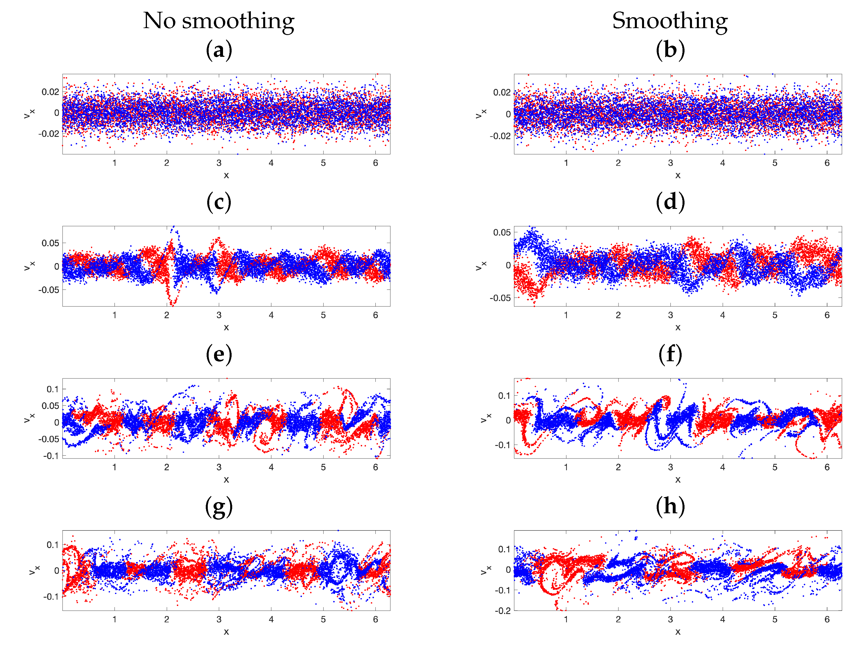
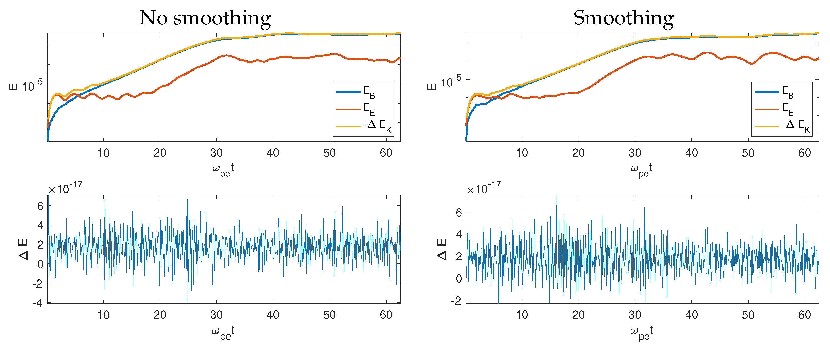
First, a method to introduce smoothing to reduce noise while retaining exact energy conservation is described. Smoothing is an affordable way to effectively introduce a higher-order interpolation scheme. It removes the high frequency part of the spectrum. Without special attention, smoothing will tend to break energy conservation by just removing high-frequency fluctuations from the system. Instead, a method that conserves energy is presented.

Second, sub-cycling is a convenient approach in plasma simulations to address the faster scales seen by the particles. In some applications, the particle response (or that of a subset of the particle population) is faster than the evolution of the fields, and it is beneficial to move the particles several times without advancing the fields. In explicit PIC, the operation is straightforward since fields and particles are not advanced together. In implicit and semi-implicit PIC, instead, sub-cycling also needs to be done in the coupling, requiring the modification of the algorithm to compute the current used in the field solution.

Finally, we illustrate how the mass matrix formulation opens up the opportunity to approximate the mass matrix in certain limit cases to reduce the cost of the simulation.

The paper is organized as follows. Section 2 recaps the key properties of the ECsim needed for the discussion. Section 3 introduces how smoothing can be implemented to reduce noise while retaining the property of energy conservation. Section 4 is dedicated to the algorithm for sub-cycling the particle motion within the ECsim scheme. Section 5 derives a limit case of the mass matrix formulation that transforms the ECsim algorithm into the standard implicit moment method [9]. Results are presented in Section 6, and final conclusions are drawn in Section 7.

2. Summary of the ECsim Method

The ECsim method [1] is based on a formulation of the mover similar to the classic leap-frog scheme:

$$\begin{array}{c}{\displaystyle {\mathbf{x}}_p^{n+1/2}={\mathbf{x}}_p^{n-1/2}+\mathsf{\Delta }t{\mathbf{v}}_p^n,}\\ \\ {\displaystyle {\mathbf{v}}_p^{n+1}={\mathbf{v}}_p^n+\frac{q_p\mathsf{\Delta }t}{m_p}\left({\mathbf{E}}^{n+\theta }({\mathbf{x}}_p^{n+1/2})+{\overline{\mathbf{v}}}_p\times {\mathbf{B}}^n({\mathbf{x}}_p^{n+1/2})\right),}\end{array}$$

(1)

where ${\mathbf{x}}_p$ denotes the particle (labeled with p index) space position, ${\mathbf{v}}_p$ the particle velocity, $q_p$ is particle charge, $m_p$ is the particle mass, n denotes the number of a particle, and $\mathbf{E}$ and $\mathbf{B}$ are electrical and magnetic fields, respectively, ${\overline{\mathbf{v}}}_p=({\mathbf{v}}_p^{n+1}+{\mathbf{v}}_p^n)/2$ is the averaged speed, and ${\mathbf{E}}^{n+\theta }=\theta {\mathbf{E}}^{n+1}+(1-\theta ){\mathbf{E}}^n$.

This mover differs from both the explicit leap-frog mover [20] and the implicit $\theta$-mover [21]: it combines the first equation from the explicit mover with the second equation from the implicit mover, but with an important difference: the electric and magnetic fields are computed at the known position ${\mathbf{x}}_p^{n+1/2}$ rather than at the unknown position ${\overline{\mathbf{x}}}_p$. The important consequence is that the particle equations can be solved directly without any iteration needed among themselves. Instead, in the standard $\theta$-mover, a predictor-corrector iteration is required. Yet, the mover is still implicit because the new fields are not known until the field equations are solved. The ECsim method retains the coupling between advanced fields and advanced particles, requiring the solution of a linear coupled system. However, the mover itself does not require any iteration, a substantial simplification.

In the ECsim scheme, the electric and magnetic fields are computed at the known position ${\mathbf{x}}_p^{n+1/2}$. In the $\theta$-scheme, instead, they are computed at the unknown position ${\overline{\mathbf{x}}}_p$. These two positions are conceptually the same; they express the particle position at the mid-time between the old and new evaluations of the velocity. However, one is computed explicitly, in the leap-frog sense, while the other is computed as part of a predictor-corrector iteration [22,23]. Both methods are second-order accurate, but the ECsim scheme is simpler to compute. This simplicity is not just a virtue in itself but leads to an important consequence: the simplicity allows us to formulate the coupling with the fields in a way that insures exact energy conservation without requiring non-linear iterations. The $\theta$-scheme can be made energy conserving but at the cost of a fully non-linear iteration requiring a non-linear solver [2,3].The ECsim scheme allows exact energy conservation without requiring any non-linear iteration.

The properties of stability are determined by the field-particle coupling, and in this sense, the method is still implicit. For this reason, not requiring any non-linear iteration but still requiring a liner solver to deal with the field-particle coupling, the method is semi-implicit. This nomenclature is to distinguish it from the fully implicit method that requires the non-linear iteration.

Note that the force term is expressed using the magnetic field, ${\mathbf{B}}^n({\mathbf{x}}_p^{n+1/2})$, at the initial time level, but the electric field is considered at the advanced intermediate level: ${\mathbf{E}}^{n+\theta }({\mathbf{x}}_p^{n+1/2})$. The reason for this choice is simplicity and the fact that the magnetic field does no work and using the old time level does not introduce any loss of energy conservation.

The coupling of particles and fields requires us to interpolate the fields to the particle positions:

$$\begin{array}{cc}\hfill {\mathbf{E}}_p^{n+\theta }& ={\mathbf{E}}^{n+\theta }({\mathbf{x}}_p^{n+1/2})=\sum _g{\mathbf{E}}_g^{n+\theta }W({\mathbf{x}}_p^{n+1/2}-{\mathbf{x}}_g),\hfill \end{array}$$

(2)

$$\begin{array}{cc}\hfill {\mathbf{B}}_p^n& ={\mathbf{B}}^{n+\theta }({\mathbf{x}}_p^{n+1/2})=\sum _g{\mathbf{B}}_g^{n}W({\mathbf{x}}_p^{n+1/2}-{\mathbf{x}}_g).\hfill \end{array}$$

(3)

A generic index g is used for the grid. In the specific implementation within the iPic3D code [24,25], the electric field and magnetic field are not colocated, and g labels either centers (for $\mathbf{B}$) or vertices (for $\mathbf{E}$). Here, the notation is simplified: ${\mathbf{B}}_p^n\equiv {\mathbf{B}}^n({\mathbf{x}}_p^{n+1/2})$ and ${\mathbf{E}}_p^{n+\theta }\equiv {\mathbf{E}}^{n+\theta }({\mathbf{x}}_p^{n+1/2})$. In the implementation here, the interpolation function, W, is a b-spline of order $\ell =1$ [26]:

$$W({\mathbf{x}}_p-{\mathbf{x}}_g)=b_{\ell }(x_p-x_g)b_{\ell }(y_p-y_g)b_{\ell }(z_p-z_g).$$

(4)

This expression reduces trivially in 1D (one-dimensional) for the examples reported below.

For Maxwell’s equation, the standard $\theta$-scheme [24] is used:

$$\begin{array}{c}{\displaystyle {\nabla }_g\times {\mathbf{E}}^{n+\theta }+\frac{1}{c}\frac{{\mathbf{B}}_g^{n+1}-{\mathbf{B}}_g^n}{\mathsf{\Delta }t}=0,}\\ \\ {\displaystyle {\nabla }_g\times {\mathbf{B}}^{n+\theta }-\frac{1}{c}\frac{{\mathbf{E}}_g^{n+1}-{\mathbf{E}}_g^n}{\mathsf{\Delta }t}=\frac{4\pi }{c}{\overline{\mathbf{J}}}_g.}\end{array}$$

(5)

The spatial operators in Equation (5) are discretized on the grid labeled by g introduced above.

The coupling of the field equations with the particles is expressed by the current for each species:

$${\overline{\mathbf{J}}}_{sg}=\frac{1}{V_g}\sum _{p\in s}{q}_p{\overline{\mathbf{v}}}_{p}W({\mathbf{x}}_p^{n+1/2}-{\mathbf{x}}_g),$$

(6)

where the summation is over the particles of the same species, labeled by s, and $V_g$ is the cell volume.

As with the $\theta$-mover, the velocity equation can be rewritten in the equivalent form [27],

$${\overline{\mathbf{v}}}_p={\widehat{\mathbf{v}}}_p+{\beta }_s{\widehat{\mathbf{E}}}_p,$$

(7)

with

$$\begin{array}{c}{\widehat{\mathbf{v}}}_p={\alpha }_p^n{\mathbf{v}}_p^n,\\ \\ {\widehat{\mathbf{E}}}_p={\alpha }_p^n,{\mathbf{E}}_p^{n+\theta }\end{array}$$

(8)

and the rotation matrix ${\alpha }_p^n$ given by

$${\alpha }_p^n=\frac{1}{1+{\left({\beta }_s{B}_p^n\right)}^2}\left(\mathbb{I}-{\beta }_s\mathbb{I}\times {\mathbf{B}}_p^n+{\beta }_s^2{\mathbf{B}}_p^n{\mathbf{B}}_p^n\right),$$

(9)

where $\mathbb{I}$ is the dyadic tensor (a matrix with a diagonal of 1) and ${\beta }_s=q_p\mathsf{\Delta }t/2m_p$ (independent of the particle weight and unique to a given species). The elements of the rotation matrix are indicated as ${\alpha }_p^{ij,n}$, with labels i and j referring to the 3 components of the vector space (x, y, z).

Substituting Equation (7) into Equation (6), one obtains without any approximation or linearization,

$${\overline{\mathbf{J}}}_{sg}=\frac{1}{V_g}\sum _p{q}_p{\widehat{\mathbf{v}}}_p{W}_{pg}+\frac{{\beta }_s}{V_g}\sum _p{q}_p{\widehat{\mathbf{E}}}_p^{n+\theta }{W}_{pg},$$

(10)

where the notation is shortened, $W_{pg}=W({\mathbf{x}}_p^{n+1/2}-{\mathbf{x}}_g)$, and the summation is intended over all particles of species s.

Using Equation (8), the expression for the current becomes

$${\overline{\mathbf{J}}}_{sg}={\widehat{\mathbf{J}}}_{sg}+\frac{{\beta }_s}{V_g}\sum _p{q}_p{\alpha }_p^n{\mathbf{E}}_p^{n+\theta }{W}_{pg},$$

(11)

where

$${\widehat{\mathbf{J}}}_{sg}=\frac{1}{V_g}\sum _p{q}_p{\widehat{\mathbf{v}}}_p{W}_{pg}.$$

(12)

Computing then the electric field on the particles by interpolation form the grid as in Equation (3), it follows that

$${\overline{\mathbf{J}}}_{sg}={\widehat{\mathbf{J}}}_{sg}+\frac{{\beta }_s}{V_g}\sum _p\sum _{g^{\prime }}{q}_p{\alpha }_p^n{\mathbf{E}}_{g^{\prime }}^{n+\theta }{W}_{p{g}^{\prime }}{W}_{pg}.$$

(13)

Exchanging the order of summation, one obtains:

$${\overline{\mathbf{J}}}_{sg}={\widehat{\mathbf{J}}}_{sg}+\frac{{\beta }_s}{V_g}\sum _{g^{\prime }}{M}_{s,g{g}^{\prime }}{\mathbf{E}}_{g^{\prime }}^{n+\theta },$$

(14)

where the actor in the leading role of the ECsim scheme—the mass matrix [28] is defined:

$$M_{s,g{g}^{\prime }}^{ij}=\sum _p{q}_p{\alpha }_p^{ij,n}{W}_{p{g}^{\prime }}{W}_{pg}.$$

(15)

There are $3v$ (where v is the number of velocity directions) mass matrices, and in matrix notation, they can be written as $M_{g{g}^{\prime }}$, that is, without the indices $i,j$ for the vector directions.

The mass matrices $M_{s,g{g}^{\prime }}$ are the most important aspect of the ECsim method and are also the most expensive part of the computation [25]. A number of symmetries can be used to reduce the cost. Speeding up the construction can be achieved using offloading to accelerator processors (e.g., graphical processing units, GPU) [29]. The mass matrices, as shown in Equation (14), provide an explicit linear link between the advanced current at the mid-point of the time step and the electric field at the advanced time. This linear relationship can be substituted into the discretized Maxwell’s Equation (5) to form a linear set of equations:

$$\left\{\begin{array}{c}{\displaystyle {\nabla }_g\times {\mathbf{E}}^{n+\theta }+\frac{1}{c}\frac{{\mathbf{B}}^{n+1}-{\mathbf{B}}^n}{\mathsf{\Delta }t}=0,}\hfill \\ \\ {\displaystyle {\nabla }_g\times {\mathbf{B}}^{n+\theta }-\frac{1}{c}\frac{{\mathbf{E}}^{n+1}-{\mathbf{E}}^n}{\mathsf{\Delta }t}=\frac{4\pi }{c}\left({\widehat{\mathbf{J}}}_g+\sum _{g^{\prime }}{M}_{g{g}^{\prime }}{\mathbf{E}}_{g^{\prime }}^{n+\theta }\right),}\hfill \end{array}\right.$$

(16)

where the total current is ${\widehat{\mathbf{J}}}_g={\sum }_s{\widehat{\mathbf{J}}}_{sg}$, and the species summed mass matrices that are written by elements are:

$$M_{g{g}^{\prime }}^{ij}=\sum _s\frac{{\beta }_s}{V_g}{M}_{s,g{g}^{\prime }}^{ij}.$$

(17)

The direct link provided by the mass matrix is analytically exact for the original set of discretized equations. Unlike the implicit moment method, where the equations have to be approximated by Taylor series expansion [27], here, the link is still exactly the same as in the original set of discretized equations. Having eliminated the need for any approximation or Taylor series expansion is the reason why ECsim conserves energy exactly.

Let us consider now how energy conservation can be shown in the case $\theta =1/2$. This is important for the derivations below to consider what key steps enable energy conservation.

The inner product of the velocity from Equation (1) with the average speed, ${\overline{\mathbf{v}}}_p$, gives, by summing over all particles,

$$\frac{1}{2}\sum _p\left(m_p{\left({\mathbf{v}}_p^{n+1}\right)}^2-{\left({\mathbf{v}}_p^n\right)}^2\right)=\mathsf{\Delta }t\sum _p\left(q_p\sum _g{\overline{\mathbf{v}}}_p·{\overline{\mathbf{E}}}_g{W}_{pg}\right),$$

(18)

where the electric field is computed as an average consistent with the choice $\theta =1/2$, and the magnetic field drops out as obvious from the properties of the cross-product.

Exchanging the summation over particles and cells leads to:

$$\frac{1}{2}\sum _p\left(m_p{\left({\mathbf{v}}_p^{n+1}\right)}^2-{\left({\mathbf{v}}_p^n\right)}^2\right)=\mathsf{\Delta }t\sum _g{\overline{\mathbf{J}}}_g·{\overline{\mathbf{E}}}_g,$$

(19)

where it is recognized that ${\overline{\mathbf{J}}}_g={\sum }_p{q}_p{\overline{\mathbf{v}}}_p{W}_{pg}$.

Multiplying the first Equation (5) by ${\overline{\mathbf{B}}}_g$ and the second by ${\overline{\mathbf{E}}}_g$ and summing them leads to:

$$\begin{array}{c}{\displaystyle \frac{{\left({\mathbf{B}}_g^{n+1}\right)}^2-{\left({\mathbf{B}}_g^n\right)}^2}{2c}+\frac{{\left({\mathbf{E}}_g^{n+1}\right)}^2-{\left({\mathbf{E}}_g^n\right)}^2}{2c}}\hfill \\ \\ {\displaystyle =\mathsf{\Delta }t\left(\frac{4\pi }{c}{\overline{\mathbf{J}}}_g·{\overline{\mathbf{E}}}_g+{\mathbf{E}}_g·{\nabla }_g\times \mathbf{B}-{\mathbf{B}}_g·{\nabla }_g\times \mathbf{E}\right).}\hfill \end{array}$$

(20)

Assuming a mimetic grid discretization that preserves the continuum properties of the operators and summing over all grid points gives:

$$\begin{array}{c}{\displaystyle \sum _g\frac{{\left({\mathbf{B}}_g^{n+1}\right)}^2-{\left({\mathbf{B}}_g^n\right)}^2}{4\pi }+\sum _g\frac{{\left({\mathbf{E}}_g^{n+1}\right)}^2-{\left({\mathbf{E}}_g^n\right)}^2}{4\pi }}\hfill \\ \\ {\displaystyle =\mathsf{\Delta }t\sum _g{\overline{\mathbf{J}}}_g·{\overline{\mathbf{E}}}_g+\frac{c\mathsf{\Delta }t}{4\pi }\sum _g{\nabla }_g·({\mathbf{E}}_g\times {\mathbf{B}}_g).}\hfill \end{array}$$

(21)

This conservation law states that the variation of the magnetic and electric energy, as measured on the grid, equals the amount exchanged with the particles and carried by the grid-discretized divergence of the Poynting flux. For energy to be conserved in the system, the energy exchange term on the particle equations (Equation (19)) needs to be identical to that on the field equations, (Equation (21)). This term is indeed identically equal to ${\sum }_g{\overline{\mathbf{J}}}_g·{\overline{\mathbf{E}}}_g$ in both equations. Energy conservation is enforced exactly to round off.

In addition to guaranteeing physical conservation of energy, a cornerstone in any physical model, the existence of this conservation constraint also guarantees a form of non-linear stability of the discretized equations [1], expanding the stability of the semi-implicit method compared with the moment implicit scheme [11,16].

3. Smoothing with the Mass Matrix Formulation

Smoothing can be designed to be compatible with the energy conserving properties of the mass matrix. Only the electric field is chosen to be smoothed, since the magnetic field tends to be much smoother in PIC simulations and smoothing is not needed.

From the proof of energy conservation recapped above, it is clear that for energy conservation, the smoothing of the current must be done in the same way as that of the electric field in the mover. Starting from the mover and calling ${\mathbb{S}}_{g{g}^{\prime }}$ the smoothing operator, a smoothed electric field on the grid is defined as:

$${\mathbf{E}}_g^{SM}=\sum _{g^{\prime }}{\mathbb{S}}_{g{g}^{\prime }}{\mathbf{E}}_{g^{\prime }}^{n+\theta }.$$

(22)

From Equation (22), the smoothed electric field acting on a particle can be computed as:

$${\mathbf{E}}_p^{SM}=\sum _g{\mathbf{E}}_g^{SM}W({\mathbf{x}}_p^{n+1/2}-{\mathbf{x}}_g).$$

(23)

The second equation of motion, Equation (1), then uses the smoothed electric field as:

$${\mathbf{v}}_p^{n+1}={\mathbf{v}}_p^n+\frac{q_p\mathsf{\Delta }t}{m_p}\left({\mathbf{E}}_p^{SM}+{\overline{\mathbf{v}}}_p\times {\mathbf{B}}_p^n\right),$$

(24)

where ${\mathbf{B}}_p^n$ is still computed as above.

From Equation (24), one can again compute the current as

$${\overline{\mathbf{J}}}_{sg}={\widehat{\mathbf{J}}}_{sg}+\frac{{\beta }_s}{V_g}\sum _{g^{\prime }}{M}_{s,g{g}^{\prime }}{\mathbf{E}}_{g^{\prime }}^{SM}.$$

(25)

The energy exchange term for the particles then becomes

$$\frac{1}{2}\sum _p\left(m_p{\left({\mathbf{v}}_p^{n+1}\right)}^2-{\left({\mathbf{v}}_p^n\right)}^2\right)=\mathsf{\Delta }t\sum _s\sum _g\left({\widehat{\mathbf{J}}}_{sg}+\frac{{\beta }_s}{V_g}\sum _{g^{\prime }}{M}_{s,g{g}^{\prime }}{\mathbf{E}}_{g^{\prime }}^{SM}\right)·{\mathbf{E}}_g^{SM}.$$

(26)

Applying smoothing to the source term of the second of the Maxwell Equation (16), one obtains:

$${\nabla }_g\times {\mathbf{B}}^{n+\theta }-\frac{1}{c}\frac{{\mathbf{E}}_g^{n+1}-{\mathbf{E}}_g^n}{\mathsf{\Delta }t}=\frac{4\pi }{c}\sum _s\sum _{g^{\prime }}{\mathbb{S}}_{g{g}^{\prime }}\left({\widehat{\mathbf{J}}}_{s{g}^{\prime }}+\frac{{\beta }_s}{V_g}\sum _{g^{″}}{M}_{s,g^{\prime }{g}^{″}}{\mathbf{E}}_{g^{″}}^{SM}\right),$$

(27)

where the last term is expressed from Equation (25).

For the fields, the energy integral then becomes:

$$\begin{array}{c}{\displaystyle \sum _g\frac{{\left({\mathbf{B}}_g^{n+1}\right)}^2-{\left({\mathbf{B}}_g^n\right)}^2}{4\pi }+\sum _g\frac{{\left({\mathbf{E}}_g^{n+1}\right)}^2-{\left({\mathbf{E}}_g^n\right)}^2}{4\pi }-\frac{c\mathsf{\Delta }t}{4\pi }\sum _g{\nabla }_g·({\mathbf{E}}_g\times {\mathbf{B}}_g)}\hfill \\ \\ {\displaystyle =\mathsf{\Delta }t\sum _s\sum _g\sum _{g^{\prime }}{\mathbb{S}}_{g{g}^{\prime }}\left({\widehat{\mathbf{J}}}_{s{g}^{\prime }}+\frac{{\beta }_s}{V_{g^{\prime }}}\sum _{g^{″}}{M}_{s,g^{\prime }{g}^{″}}{\mathbf{E}}_{g^{″}}^{SM}\right)·{\overline{\mathbf{E}}}_g.}\hfill \end{array}$$

(28)

For the two energy integrals to be the same, the exchange term seen by the particles must be equal to that seen by the fields. The right-hand sides of Equation (26) must then equal that of Equation (28):

$$\begin{array}{c}\hfill \sum _g\sum _{g^{\prime }}{\mathbb{S}}_{g{g}^{\prime }}\left({\widehat{\mathbf{J}}}_{s{g}^{\prime }}+\frac{{\beta }_s}{V_{g^{\prime }}}\sum _{g^{″}}{M}_{s,g^{\prime }{g}^{″}}{\mathbf{E}}_{g^{″}}^{SM}\right)·{\overline{\mathbf{E}}}_g\\ \hfill =\sum _g\left({\widehat{\mathbf{J}}}_{sg}+\frac{{\beta }_s}{V_g}\sum _{g^{″}}{M}_{s,g{g}^{″}}{\mathbf{E}}_{g^{″}}^{SM}\right)·\sum _{g^{\prime }}{\mathbb{S}}_{g{g}^{\prime }}{\overline{\mathbf{E}}}_{g^{\prime }}.\end{array}$$

(29)

Switching g with $g^{\prime }$ (just names) in the right-hand side, the equivalence above holds when the smoothing operator is symmetric (i.e., the matrix repenting it is symmetric), a common property shared by many smoothing operators [3].

Note that the electric field is smoothed but not the magnetic field, which tends to be less noisy by its nature.

4. Sub-Cycling with the Mass Matrix Formulation

A mass matrix can also be defined in the presence of sub-cycling or orbit-averaging movers. The velocity update of ECsim can be reformulated for sub-cycling as

$${\displaystyle {\mathbf{v}}_p^{\nu +1}={\mathbf{v}}_p^{\nu }+\frac{q_p\mathsf{\Delta }{t}_{\nu }}{m_p}\left({\mathbf{E}}^{n+\theta }\left({\mathbf{x}}_p^{\nu }\right)+\frac{{\mathbf{v}}_p^{\nu +1}+{\mathbf{v}}_p^{\nu }}{2}\times {\mathbf{B}}^n\left({\mathbf{x}}_p^{\nu }\right)\right).}$$

(30)

It is assumed assume that the time step $\mathsf{\Delta }t$ between field updates is subdivided into $N_{\nu }$, not necessarily equal sub-steps $\mathsf{\Delta }{t}_{\nu }$.

The positions for the field evaluations, ${\mathbf{x}}_p^{\nu }$, during the sub-cycle can be computed in different ways. The simplest is to assume a straight orbit within $\mathsf{\Delta }t$, similar to the leap-frog approach:

$${\mathbf{x}}_p^{\nu }={\mathbf{x}}_p^{n-1/2}+{\mathbf{v}}_p^n\sum _{{\nu }^{\prime }=0}^{{\nu }^{\prime }=\nu }\mathsf{\Delta }{t}_{{\nu }^{\prime }},$$

(31)

which can all be computed at once since the same velocity is used for all points along the trajectory. The first step starts from the old position ${\mathbf{x}}_p^{\nu =0}={\mathbf{x}}_x^n$ and old velocity ${\mathbf{v}}_p^{\nu =0}={\mathbf{v}}_x^n$, and the last step leads to the final position ${\mathbf{x}}_p^{\nu =N_{\nu }}={\mathbf{x}}_p^{n+1}$ and final velocity ${\mathbf{v}}_p^{\nu =N_{\nu }}={\mathbf{v}}_p^{n+1}$. The fields are assumed to be those computed at the time level $\theta$ within the field update time step $\mathsf{\Delta }t$.

Another promising approach is to recall that most often in plasma physics, particles are not moving in straight lines, but rather they are frozen into the field lines, moving in cyclotron orbits with drifts due to the inhomogeneity of the fields. In the spirit of gyro-averaging, certain applications of the implicit method might need to step over the gyration time scale, and the positions of the particles used in Equation (30) would then be chosen to achieve accurate gyro-averaging, for example taking $N_{\nu }$ positions along the gyro-orbit of a particle [30] to compute an average force on the particle’s center of gyration.

The example of the two strategies above for computing the intermediate positions can be made in a single explicit step that generates all positions at once: in this case, each substep contribution to the mass matrix and the moments can be computed in parallel, greatly improving the parallel performance. In practice, the $N_{\nu }$ operations required by the substepping algorithm can all be done in parallel in an embarrassingly parallel approach that scales ideally on supercomputers: no communication between the particles and between the substeps is needed.

Equation (30) can be inverted with the same vector manipulations used for Equation (1) to obtain:

$$\frac{{\mathbf{v}}_p^{\nu +1}+{\mathbf{v}}_p^{\nu }}{2}={\widehat{\mathbf{v}}}_p^{\nu }+{\beta }_s{\widehat{\mathbf{E}}}_p^{\nu },$$

(32)

where hatted quantities have been rotated by the magnetic field computed at the location ${\mathbf{x}}_p^{\nu }$:

$$\begin{array}{c}{\widehat{\mathbf{v}}}_p^{\nu }={\alpha }_p^{\nu }{\mathbf{v}}_p^{\nu },\\ \\ {\widehat{\mathbf{E}}}_p^{\nu }={\alpha }_p^{\nu }{\mathbf{E}}^{n+\theta }\left({\mathbf{x}}_p^{\nu }\right),\end{array}$$

(33)

via a rotation matrix, ${\alpha }_p^n$, defined as in the case of a singe step, but with the magnetic field computed at the last substep position:

$${\alpha }_p^{\nu }=\frac{1}{1+{\left({\beta }_s{B}^n\left({\mathbf{x}}_p^{\nu }\right)\right)}^2}\left(\mathbb{I}-{\beta }_s\mathbb{I}\times {\mathbf{B}}^n\left({\mathbf{x}}_p^{\nu }\right)+{\beta }_s^2{\mathbf{B}}^n\left({\mathbf{x}}_p^{\nu }\right){\mathbf{B}}^n\left({\mathbf{x}}_p^{\nu }\right)\right).$$

(34)

From Equation (32), one can obtain directly from its definition (6) the mean current over all sub-steps without any further approximation or linearization:

$${\overline{\mathbf{J}}}_{sg}=\frac{1}{V_g}\sum _p{q}_p\sum _{\nu }\frac{\mathsf{\Delta }{t}_{\nu }}{\mathsf{\Delta }t}\left({\widehat{\mathbf{v}}}_p^{\nu }+{\beta }_s{\widehat{\mathbf{E}}}_p^{\nu }\right)W_{pg}^{\nu },$$

(35)

where $W_{pg}^{\nu }=W({\mathbf{x}}_p^{\nu }-{\mathbf{x}}_g)$. Using now the definitions of the hatted quantities, Equation (33), one can cast the mean current in the same form as in the single step formulation:

$${\overline{\mathbf{J}}}_{sg}={\widehat{\mathbf{J}}}_{sg}+\frac{{\beta }_s}{V_g}\sum _{g^{\prime }}{M}_{s,g{g}^{\prime }}{\mathbf{E}}_{g^{\prime }}^{n+\theta },$$

(36)

but with the new definition for

$${\widehat{\mathbf{J}}}_{sg}=\frac{1}{V_g}\sum _p{q}_p\sum _{\nu }\frac{\mathsf{\Delta }{t}_{\nu }}{\mathsf{\Delta }t}{\widehat{\mathbf{v}}}_p^{\nu }{W}_{pg}^{\nu }.$$

(37)

and the mass matrix for a sub-cycled trajectory defined by

$$M_{s,g{g}^{\prime }}^{ij}=\sum _p{q}_p\sum _{\nu }\frac{\mathsf{\Delta }{t}_{\nu }}{\mathsf{\Delta }t}{\alpha }_p^{ij,\nu }{W}_{p{g}^{\prime }}^{\nu }{W}_{pg}^{\nu }.$$

(38)

Note that the definition of the sub-cycled mass matrix (Equation (38)) and the sub-cycled hatted current (Equation (37)) treats each sub-interval for each particle as if they were independent: the equations see each sub-interval as a particle. It is as if the system has $N_p{N}_{\nu }$ particles made by each particle for each sub-interval ${\mathsf{\Delta }}_{\nu }$. This feature lends itself to a simpler computing implementation where each particle is spawned into $N_{\nu }$ treated as independent particles in the interpolation, mass matrix computation and current gathering step. This is a valuable approach in parallel and vectorized computer architectures, such as GPUs.

Regardless of how the positions for the particles during the sybcycling are chosen, if the current defined in Equation (36) is computed with the mass matrices defined in Equation (38), energy is conserved. In fact, the term ${\sum }_g{\overline{\mathbf{J}}}_g·{\overline{\mathbf{E}}}_g$ is again identical when computed from the equations for the particles and for the fields.

5. Simplification of the Mass Matrix: The Limit of the Implicit Moment Method

There is a specific case where the mass matrix formulation takes a much simplified form: in the case of the interpolation of the nearest grid point (NGP). In that case, the interpolation function $W_{pg}$ is simple: 1 for the nearest grid point, which is labeled here as $g_p$, and 0 for everywhere else:

$$W_{pg}={\delta }_{g_{p}g},$$

(39)

where ${\delta }_{ab}$ is the Kronecker delta.

In this case, the mass matrix becomes

$$M_{s,g{g}^{\prime }}^{ij}=\sum _p{q}_p{\alpha }_p^{ij,n}{\delta }_{g_p{g}^{\prime }}{\delta }_{g_{p}g}.$$

(40)

When substituted in the expression for the current, this leads to

$${\overline{\mathbf{J}}}_{sg}={\widehat{\mathbf{J}}}_{sg}+\frac{{\beta }_s}{V_g}\sum _p\sum _{g^{\prime }}{q}_p{\alpha }_p^n{\mathbf{E}}_{g^{\prime }}^{n+\theta }{\delta }_{g_p{g}^{\prime }}{\delta }_{g_{p}g}.$$

(41)

Given the properties of Kronecker delta, the summation over $g^{\prime }$ can be done first:

$$\sum _{g^{\prime }}{\mathbf{E}}_{g^{\prime }}^{n+\theta }{\delta }_{g_p{g}^{\prime }}={\mathbf{E}}_{g_p}^{n+\theta },$$

(42)

and substituting:

$${\overline{\mathbf{J}}}_{sg}={\widehat{\mathbf{J}}}_{sg}+\frac{{\beta }_s}{V_g}\sum _p{q}_p{\alpha }_{g_p}^n{\mathbf{E}}_{g_p}^{n+\theta }{\delta }_{g_{p}g},$$

(43)

where the point that the $\alpha$s are computed using the magnetic fields of the nearest grid point is used, consistent with the NGP interpolation. Using again the properties of Kronecker delta, the summation over the particles can be done directly:

$$\frac{1}{V_g}\sum _p{q}_p={\rho }_{sg},$$

(44)

to obtain

$${\overline{\mathbf{J}}}_{sg}={\widehat{\mathbf{J}}}_{sg}+{\beta }_s{\rho }_{sg}{\alpha }_g^n{\mathbf{E}}_g^{n+\theta }.$$

(45)

This is the same expression that links the electric field and the current in the implicit moment method [31] used in Venus2D [9], in Celeste3D [23] and iPic3D [24]. It is then worth considering this limit expression for the mass matrix formulation. Most often, the NGP cannot be used in practice for its well known excessive noise, but the expression (45) still can be used even in the presence of other interpolation schemes.

Equation (45) is exact only for the NGP scheme where it still leads to exact energy conservation. When, instead, other orders of interpolation are used, energy conservation is lost, but it still provides a meaningful link between the current and electric field: it is, in fact, the same used for decades by the implicit moment method. If Equation (45) is used, ECsim becomes more similar to the implicit moment method, but it still differs in one key aspect: the interpolations are computed using the position provided by the leap-frog algorithm for the particle position. This is known explicitly and does not require any iteration. In the implicit moment method, the mover requires to iterate between the velocity update and position update using a predictor-corrector scheme. This is not required in ECsim, where the particle position is known explicitly from the previous time step.

6. Results

6.1. Effects of Sub-Cycling

To check how the innovations described above perform in practice, let us first consider the effect of sub-cycling. The goal is twofold. First, one needsto verify that the energy is indeed conserved and sub-cycling does not break the energy conservation. Second, one tests on a specific case how far one can push the sub-cycling before the correctness of the results deteriorates. The first task above is just a confirmation of the rigorously exact calculations above, and it is merely a verification test for the code implemented here. The second task is only an illustration because the usefulness of sub-cycling is highly problem-dependent.

A two-stream instability was initiated by considering a domain of $L/d_e=2\pi$ divided into 64 cells with 10,000 particles. A mini-app was useful to readily study implementations in different computer architectures: it was intended merely as a test, not as a real world problem. Space was normalized in electron skin depth, $d_e=c/{\omega }_{pe}$, and time was normalized in electron plasma frequency, ${\omega }_{pe}t$. The ions were kept immobile, while the electrons had a thermal speed of $v_{\mathrm{the}}/c=0.02$ (with c denoting the speed of light), and the two beams had a net speed of $V_0/c=\pm 0.1$. The reference case without sub-cycling ($N_{\nu }=1$) has a CFL (Courant–Friedrichs–Lewy) condition Courant number, $C=V_0\mathsf{\Delta }t/\mathsf{\Delta }x=0.1$. We then proceeded to carry out 10 runs with $N_{\nu }=1$–10, and $\mathsf{\Delta }t$ was increased by the same factor. That is, the particle $\mathsf{\Delta }t$ was kept fixed and the $\mathsf{\Delta }t$ of the field was increased. As the number of sub-cycles increased, the $\mathsf{\Delta }t$ increased, but the total time remains the same: ${\omega }_{pe}t=50$. A perturbation of the particle velocity was added with mode number, $m=5$:

$$u_p=u_p+V_{1}sin\left(\frac{2\pi m{x}_p}{L}\right);$$

(46)

with an amplitude $V_1=V_0/10$.

Here, a MATLAB implementation was used that was tested on a MAC OSX 10.14.6 with an Intel Core i7 2,6GHz processor complemented with 16GB DDR3 1600 MHz memory.

The results of the study are summarized in

Table 1. Effect of sub-cycling on a two-stream instability run. Values attained while varying the number $N_{\nu }$ of sub-cycles, from 1 to 10 and correspondingly increasing the duration of the simulation in seconds, the seconds spent per the time step, $\mathsf{\Delta }t$, and the energy error, $\mathsf{\Delta }E$, by the same factor $\mathsf{\Delta }t$ are reported.

${\mathit{N}}_{\mathit{\nu }}$	Time (s)	Seconds/$\mathbf{\Delta }\mathit{t}$	$\mathbf{\Delta }\mathit{E}$
1.0	42.73	0.08395	$1.75\times {10}^{-16}$
2.0	20.94	0.08244	$1.1\times {10}^{-16}$
3.0	14.63	0.08657	$1.015\times {10}^{-16}$
4.0	10.88	0.08567	$7.388\times {10}^{-17}$
5.0	8.97	0.08881	$6.764\times {10}^{-17}$
6.0	7.36	0.08762	$8.342\times {10}^{-17}$
7.0	6.46	0.08972	$7.988\times {10}^{-17}$
8.0	5.74	0.09111	$8.492\times {10}^{-17}$
9.0	5.27	0.09411	$8.14\times {10}^{-17}$
10.0	4.79	0.0958	$8.61\times {10}^{-17}$

and in Figure 1 and Figure 2.

Table 1 reports the reduction of the cost of the simulation as the number of sub-cycles increased. The MATLAB implementation is well vectorized and efficient in handling the particle projections, so much so that as the number of sub-cycles is increased, the cost per $\mathsf{\Delta }t$ hardly increases at all. If one compares the cost of a time step without sub-cyclig (0.08395 s) with that with 10 sub-cycles (0.0958 s), the increase is minimal even though particles have been moved and projected to the moments and the construction of the mass matrix 10 times more. While this result is specific to the vectorization done via MATLAB, other forms of vectorization are also possible on GPUs using OpenACC [32] and CUDA [33] programs opening up a similar opportunity for this type of optminization in other implementations.

As required by the theoretical derivations above, energy should be conserved in all cases. This is indeed the case in Table 1, a confirmation that the MATLAB implementation used is bug-free.

However, if sub-cycling is beneficial in reducing the cost of the simulation, it introduces a degradation in the physics sense. Particles are moved with the same time step in each sub-cycle regardless of $N_{\nu }$, but as $N_{\nu }$ increases, the overall time step $\mathsf{\Delta }t$ for the field recalculation is increased. In a number of problems, it is still beneficial to accept this compromise. Figure 1 and Figure 2 show the degradation of the results with $N_{\nu }$. Unfortunately, the instability modeled is a complex non-linear process, and the linear phase is not important: an easy quantitative metric of accuracy is not available. The study was already started from a significant perturbation. If not added then several modes develop at the same time, and still, the linear phase is muddied by the interaction of many modes. There is no single metric that can easily summarize the quality of the evolution. One has to rely on qualitative visual comparison. For this reason, let us look carefully at the velocity space distribution (Figure 1) and phase space (Figure 2). As $N_{\nu }$ is increased, the correct physics description is progressively lost.

The most characteristic feature of the two-stream instability is the formation of a flat top distribution, a distribution where, for a range of velocities, the distribution remains flat. This feature is prominent without sub-cycling, and it is still reasonably well represented at higher sub-cycling numbers. However, the tail of higher-energy particles is reduced when sub-cycling is increased, a reflection of the fact that the electric field responsible for particle acceleration [34] is less accurately computed. These are non-physical artifacts of excessive sub-cycling.

The same conclusion is reached by analysing phase space. In this case, the most important feature is the formation of electron holes, regions of phase space depleted of electrons and in fact completely void of them. These features, which are also observed in experimental measurements, are distorted and expelled to the edge of the velocity range as $N_{\nu }$ is increased.

Sub-cycling is compatible with the mass matrix formulation, retaining the property of exact energy conservation. It can be implemented effectively enough, only minimally increasing the cost of the computational cycle despite the increase in the number of particle operations while reducing the number of time steps for the same total time. However, it must be used with care because not updating the fields after the particles are moved in a sub-cycle introduces physical errors even though energy is still exactly conserved.

6.2. Effects of Smoothing

To test the effects of smoothing, let us consider another type of streaming instability: the transverse electromagnetic instability driven by counter streaming beams [35]. Again, a 1D plasma (x is the only spatial variable) is considered, but now, all three components of the particle velocity are taken into account. The two counter-streaming beams are directed along $\mathbf{y}$. Using the speed of light for normalization, a case with the beams having $v_{\mathrm{the}}/c=0.01$ counter-streaming with speed $v_{0y}/c=0.2$ to be considered. No initial perturbation is added and the natural noise is let to initiate the instability. The transverse electromagnetic streaming instability is common is often used in the context of understanding how magnetic fields can be generated in the universe [36] a form of dynamo. A setup similar to that reported by Innocenti et al. [37] is used. A characteristic of this instability is that it segregates in phase space particles with opposite signs of $v_y$, initially residing in the two different beams.

Figure 3 shows the evolution of the phase space cross-section $(x,v_x)$: the red particles have $v_y<0$ and the blue particles have $v_y>0$. The evolution initially retains their separation, but in time, phase-space mixing takes over. More details of the physics of this simulation can be found by Innocenti et al. [37]. Let us focus here on comparing the normal ECsim case without smoothing with one where the smoothing kernel, $\mathbb{S}=[1/4,1/2,1/4]$, is applied by convolution 3 times. Figure 3 compares the smoothed and non-smoothed case. Smoothing does not alter the evolution in any profound ways, but it affects it. Since the simulation is started from its natural noise, no two simulations will be identical, and of course, the smoothed simulation will have less noise. The locations of the islands formed in phase space are not the same, but the overall features are similar.

The energy exchange is also similar in the smoothed and non-smoothed runs, as shown in Figure 4. In particular, the kinetic energy is lost primarily to produce magnetic energy. The transverse counter-streaming instability is a form of magnetic dynamo that spontaneously creates a magnetic field by using the kinetic energy of the counter-streaming beams. The total energy is conserved to machine precision in both runs. Smoothing, as shown in Section 3 theoretically, indeed conserves energy exactly.

The main effect of smoothing is to eliminate the high-frequency part of the spectrum. Figure 5 and Figure 6 compare the k–$\omega$ spectrum of selected fields. The noise at high values of k is reduced. The spectrum identifies the low k part of the spectrum as dominant. The characteristic arch of the electromagnetic waves (light waves) is also prominent.

7. Discussion

The ECsim method allows to make a PIC simulation within a semi-implicit approach that conserves energy exactly. This feature, besides having its own intrinsic value, also leads to improved stability, allowing, for example, to consider realistic plasma conditions in the heliosphere, including the colder solar wind where the Debye length is very small compared with the scales of interest.

This paper reports on three new developments.

First, a method for smoothing the electric field in an algorithm that preserves energy conservation is introduced. When it can be avoided, smoothing should be avoided, but when there is a need for it, the algorithm presented here achieves smoothing without breaking energy conservation. This can be, for example, the case when excessive noise alters the correct transport properties of a plasma, an issue of great importance, for example, in fusion energy studies [38].

Second, a method for computing the mass matrix in the presence of particle sub-cycling is introduced. Sub-cycling can be useful in a number of situations. Most often, if it can be avoided, it should be avoided because particles and fields move together, with the frozen-in condition being a cardinal property of plasmas. However, frozen-in properties are valid at the large scales typical of MHD. There are many situations where the fields evolve slowly while particles move quickly. For example, in gyro motion. Sub-cycling can be used together with gyroaveraging. The method presented here allows us to use sub-cycling while constructing a mass matrix that continues to preserve the exact energy conservation.

Finally, a limit case when the mass matrix calculation becomes especially simple is discussed and it is shown that, in this limit, the plasma particle response in the ECsim method becomes identical to that of the implicit moment method (IMM). This has two implications. First, it allows us to use the same code either in the full energy-conserving ECsim mode or in the less expensive IMM mode. Comparisons can then be made more readily. Second, the derivation clarifies the theoretical links between ECsim and IMM, revealing in what limit the two become identical.

These three new steps have both a theoretical significance and practical value, bringing understanding of the properties of ECsim and broadening its range of applications.

References

1. Lapenta, G. Exactly energy conserving semi-implicit particle in cell formulation. J. Comput. Phys. 2017, 334, 349–366. [Google Scholar] [CrossRef] [Green Version]
2. Markidis, S.; Lapenta, G. The energy conserving particle-in-cell method. J. Comput. Phys. 2011, 230, 7037–7052. [Google Scholar] [CrossRef] [Green Version]
3. Chen, G.; Chacón, L.; Barnes, D.C. An energy-and charge-conserving, implicit, electrostatic particle-in-cell algorithm. J. Comput. Phys. 2011, 230, 7018–7036. [Google Scholar] [CrossRef] [Green Version]
4. Birdsall, C.K.; Langdon, A.B. Plasma Physics via Computer Simulation; CRC Press/Taylor & Francis Group: Boca Raton, FL, USA, 1991. [Google Scholar] [CrossRef]
5. Bowers, K.J.; Albright, B.J.; Yin, L.; Daughton, W.; Roytershteyn, V.; Bergen, B.; Kwan, T.J.T. Advances in petascale kinetic plasma simulation with VPIC and Roadrunner. J. Phys. Conf. Ser. 2009, 180, 012055. [Google Scholar] [CrossRef]
6. Hockney, R.W.; Eastwood, J.W. Computer Simulation Using Particles; CRC Press/Taylor & Francis Group: Boca Raton, FL, USA, 1988. [Google Scholar] [CrossRef]
7. Lapenta, G. Particle simulations of space weather. J. Comput. Phys. 2012, 231, 795–821. [Google Scholar] [CrossRef]
8. Xiao, J.; Qin, H.; Liu, J. Structure-preserving geometric particle-in-cell methods for Vlasov-Maxwell systems. Plasma Sci. Technol. 2018, 20, 110501. [Google Scholar] [CrossRef] [Green Version]
9. Brackbill, J.U.; Forslund, D.W. An implicit method for electromagnetic plasma simulation in two dimensions. J. Computat. Phys. 1982, 46, 271–310. [Google Scholar] [CrossRef]
10. Langdon, A.B.; Cohen, B.I.; Friedman, A. Direct implicit large time-step particle simulation of plasmas. J. Computat. Phys. 1983, 51, 107–138. [Google Scholar] [CrossRef]
11. Lapenta, G.; Gonzalez-Herrero, D.; Boella, E. Multiple-scale kinetic simulations with the energy conserving semi-implicit particle in cell method. J. Plasma Phys. 2017, 83, 705830205. [Google Scholar] [CrossRef] [Green Version]
12. Walker, R.J.; Lapenta, G.; Berchem, J.; El-Alaoui, M.; Schriver, D. Embedding particle-in-cell simulations in global magnetohydrodynamic simulations of the magnetosphere. J. Plasma Phys. 2019, 85, 905850109. [Google Scholar] [CrossRef] [Green Version]
13. Zhou, H.; Tóth, G.; Jia, X.; Chen, Y.; Markidis, S. Embedded kinetic simulation of Ganymede’s magnetosphere: Improvements and inferences. J. Geophys. Res. Space Phys. 2019, 124, 5441–5460. [Google Scholar] [CrossRef]
14. Lapenta, G.; El Alaoui, M.; Berchem, J.; Walker, R. Multiscale MHD-kinetic PIC study of energy fluxes caused by reconnection. J. Geophys. Res. Space Phys. 2020, 125, e2019JA027276. [Google Scholar] [CrossRef]
15. Lapenta, G.; Schriver, D.; Walker, R.J.; Berchem, J.; Echterling, N.F.; El Alaoui, M.; Travnicek, P. Do we need to consider electrons’ kinetic effects to properly model a planetary magnetosphere: The case of Mercury. J. Geophys. Res. Space Phys. 2022, 127, e2021JA030241. [Google Scholar] [CrossRef]
16. Gonzalez-Herrero, D.; Micera, A.; Boella, E.; Park, J.; Lapenta, G. ECsim-CYL: Energy Conserving Semi-Implicit particle in cell simulation in axially symmetric cylindrical coordinates. Comput. Phys. Commun. 2019, 236, 153–163. [Google Scholar] [CrossRef] [Green Version]
17. Park, J.; Lapenta, G.; Gonzalez-Herrero, D.; Krall, N.A. Discovery of an electron gyroradius scale current layer: Its relevance to magnetic fusion energy, Earth’s magnetosphere, and sunspots. Front. Astron. Space Sci. 2019, 6, 74. [Google Scholar] [CrossRef] [Green Version]
18. Chen, Y.; Tóth, G. Gauss’s law satisfying energy-conserving semi-implicit particle-in-cell method. J. Comput. Phys. 2019, 386, 632–652. [Google Scholar] [CrossRef] [Green Version]
19. Campos Pinto, M.; Pagès, V. A semi-implicit electromagnetic FEM-PIC scheme with exact energy and charge conservation. J. Comput. Phys. 2022, 453, 110912. [Google Scholar] [CrossRef]
20. Boris, J.P. Relativistic plasma simulation-optimization of a hybrid code. In Proceedings of the Fourth Conference on Numerical Simulation of Plasmas, Washington, DC, USA, 2–3 November 1970; pp. 3–67. [Google Scholar]
21. Brackbill, J.U.; Cohen, B.I. (Eds.) Multiple Time Scales; Academic Press, Inc.: Orlando, FL, USA, 1985. [Google Scholar] [CrossRef]
22. Vu, H.X.; Brackbill, J.U. Accurate numerical solution of charged particle motion in a magnetic field. J. Comput. Phys. 1995, 116, 384–387. [Google Scholar] [CrossRef]
23. Lapenta, G.; Brackbill, J.U.; Ricci, P. Kinetic approach to microscopic-macroscopic coupling in space and laboratory plasmas. Phys. Plasmas 2006, 13, 055904. [Google Scholar] [CrossRef] [Green Version]
24. Markidis, S.; Lapenta, G.; Rizwan-uddin. Multi-scale simulations of plasma with iPIC3D. Math. Comput. Simul. 2010, 80, 1509–1519. [Google Scholar] [CrossRef] [Green Version]
25. Gonzalez-Herrero, D.; Boella, E.; Lapenta, G. Performance analysis and implementation details of the Energy Conserving Semi-Implicit Method code (ECsim). Comput. Phys. Commun. 2018, 229, 162–169. [Google Scholar] [CrossRef] [Green Version]
26. de Boor, C. A Practical Guide to Splines; Springer: New York, NY, USA, 1978. [Google Scholar]
27. Vu, H.X.; Brackbill, J.U. CELEST1D: An implicit, fully kinetic model for low-frequency, electromagnetic plasma simulation. Comput. Phys. Comm. 1992, 69, 253–276. [Google Scholar] [CrossRef]
28. Burgess, D.; Sulsky, D.; Brackbill, J.U. Mass matrix formulation of the FLIP particle-in-cell method. J. Comput. Phys. 1992, 103, 1–15. [Google Scholar] [CrossRef]
29. Boella, E.; Innocenti, M.E.; Bettencourt, M.; Chimeh, M.; Lapenta, G.; Parodi, P.; Shukla, N.; Spiga, F. On Adding GPU Support to the Particle-in-Cell code ECsim. OpenACC and Hackathons Summit 2022, 2 August 2022, Virtual. Available online: https://www.youtube.com/watch?v=9FK8zty8BgA (accessed on 15 December 2022).
30. Lee, W.W. Gyrokinetic particle simulation model. J. Comput. Phys. 1987, 72, 243–269. [Google Scholar] [CrossRef] [Green Version]
31. Ricci, P.; Lapenta, G.; Brackbill, J.U. A simplified implicit Maxwell solver. J. Computat. Phys. 2002, 183, 117–141. [Google Scholar] [CrossRef] [Green Version]
32. OpenACC. Available online: https://www.openacc.org/ (accessed on 15 December 2022).
33. CUDA Zone. Available online: https://developer.nvidia.com/cuda-zone (accessed on 15 December 2022).
34. Lapenta, G.; Markidis, S.; Marocchino, A.; Kaniadakis, G. Relaxation of relativistic plasmas under the effect of wave-particle interactions. Astrophys. J. 2007, 666, 949–954. [Google Scholar] [CrossRef]
35. Fried, B.D. Mechanism for instability of transverse plasma waves. Phys. Fluids 1959, 2, 337. [Google Scholar] [CrossRef]
36. Lazar, M.; Schlickeiser, R.; Wielebinski, R.; Poedts, S. Cosmological effects of Weibel-type instabilities. Astrophys. J. 2009, 693, 1133–1141. [Google Scholar] [CrossRef] [Green Version]
37. Innocenti, M.E.; Lazar, M.; Markidis, S.; Lapenta, G.; Poedts, S. Electron streams formation and secondary two stream instability onset in the post-saturation regime of the classical Weibel instability. Phys. Plasmas 2011, 18, 052104. [Google Scholar] [CrossRef] [Green Version]
38. Nevins, W.M.; Hammett, G.W.; Dimits, A.M.; Dorland, W.; Shumaker, D.E. Discrete particle noise in particle-in-cell simulations of plasma microturbulence. Phys. Plasmas 2005, 12, 122305. [Google Scholar] [CrossRef]
Figure 1. Particle velocity distribution at the end of 10 different simulations of same total duration varying the number of sub-cycles, N ν = 1 (top), 2, 3 to 10 (bottom), and correspondingly increasing time step, Δ t , by the same factor. See text for details.
Physics 05 00007 g001
Figure 2. Scatter plot of the phase space for the particles at the end of 10 different simulations of same total duration varying the number of sub-cycles, N ν = 1 (top), 2, 3 to 10 (bottom), and correspondingly increasing Δ t by the same factor. See text for details.
Physics 05 00007 g002
Figure 3. Evolution of the phase space section ( x , v x ) in the transverse counter-streaming instability. The red particles have v y < 0 , and the blue particles have v y > 0 . Three times are shown, and the left (right) panels report the non-smoothed (smoothed) run: ω p e t = 6.35 (a,b), 25 (c,d), 43.75 (e,f), and 62.5 (g,h). See text for details.
Physics 05 00007 g003
Figure 4. Evolution of the energy in the transverse counter-streaming instability without smoothing (left) and with smoothing (right) with the exchange between kinetic and magnetic energy, with a minority contribution going to the electric field energy (top) and the total energy conservation (bottom).
Physics 05 00007 g004
Figure 5. Transverse counter-streaming instability in absence of smoothing for E x (left,) E z (middle), and B y (right) in the spatiotemporal plane ( x , t ) (top) and in the spectral plane ( k , ω ) (bottom). See text for details.
Physics 05 00007 g005
Figure 6. Transverse counter-streaming instability in presence of smoothing. Three fields are shown from left to right: E x , E z and B y . The top row shows the spatiotemporal plane ( x , t ) , and the bottom row shows the spectral plane ( k , ω ) . E x (left), E z (middle), and B y (right) in the spatiotemporal plane ( x , t ) (top) and in the spectral plane ( k , ω ) (bottom).
Physics 05 00007 g006