Article

Damping and Dispersion of Non-Adiabatic Acoustic Waves in a High-Temperature Plasma: A Radiative-Loss Function

Department of Theoretical Physics, Kalmyk State University, Pushkin’s st., 11, Elista 358000, Russia
*
Author to whom correspondence should be addressed.
Physics 2023, 5(1), 215-228; https://doi.org/10.3390/physics5010017
Submission received: 2 December 2022 / Revised: 29 January 2023 / Accepted: 30 January 2023 / Published: 15 February 2023

Abstract

:
The behavior of acoustic waves in a rarefied high-temperature plasma is studied; as an example, the plasma of the solar corona is considered. Effects of thermal conductivity and a heating/radiative loss are taken into account; data on a temperature distribution of a radiation intensity obtained from the CHIANTI 10 code are used. The classical Spitzer expression for a full-ionized plasma is used for the thermal conductivity. Based on the found values of the radiation-loss function, the cubic spline method is used to construct an approximate analytical expression necessary for studying linear waves. A dispersion relation is obtained, and a frequency, a phase speed, and a damping coefficient are found. Dispersion and damping properties are considered for a temperature of about 10 6 K and a particle density of about 10 15 m 3 , which are typical for the coronal plasma. In sum, superiority in the dispersion and damping of the thermal conduction is shown; the heating and radiation loss manifest themselves at large wavelengths. In accordance with general results by Field, a condition was found under which the acoustic oscillations become unstable. It is shown that at certain values of the temperature and density, the wave damping is dominated by the heating/radiative loss misbalance. Thus, the earlier results on mechanisms of damping of observed acoustic waves in the solar corona are refined here.

1. Introduction

A study of acoustic waves, which are observed all over in the lower corona by variations in the intensity of plasma radiation in various electromagnetic ranges, plays an important role in solar research [1,2,3,4,5]. Acoustic waves can provide useful information about parameters of the coronal plasma [6,7] or indicate sources of its heating. In the latter case, the mechanism and efficiency of wave energy dissipation are of interest. In a rarefied high-temperature coronal plasma, the role of viscous dissipation is insignificant [8,9], so wave damping due to thermal conductivity is more often taken into account. At the same time, it was noticed that, along with thermal conductivity, damping of loop oscillations in the corona can be noticeably affected by radiative loss [10,11]. Radiation affects slow magnetoacoustic oscillations more than fast ones [12]. This is explained by the fact that under conditions of the solar corona, where the Alfvén speed significantly exceeds the sound speed, slow waves are practically longitudinal. For this reason, slow waves are sometimes considered approximately as acoustic.
The study of the damping of acoustic waves in high-temperature coronal plasma in recent years has been carried out while taking into account the effects of thermal conduction and heating/radiative loss [13,14,15]. We follow this approach in the present study. Absorption leads not only to the damping of the acoustic wave, but also to its dispersion [16]. This should lead to the appearance of quasi-periodic oscillations generated as a result of the spreading of an initial localized perturbation. A misbalance between heating and radiative loss has a similar effect on the wave [14]. A goal of this study is to compare both the effects of thermal conductivity and heating/cooling on the damping and dispersion of the acoustic wave. Unlike other similar studies, which are based on general assumptions about the properties of plasma heating and radiation, we use the established values of the radiative-loss function obtained using the the CHIANTI [17,18,19] code.
We built an approximate analytical representation of the radiative-loss function by cubic spline interpolation. This is then used in the analysis of a linear acoustic wave. This allows one, together with the known expression for the thermal conductivity of a highly-ionized high-temperature plasma, to determine the specific physical conditions for the wave and compare the results of the analysis with observational data. The definiteness of the physical model makes it possible to estimate the parameters of the coronal plasma, which is the main task of coronal seismology.
We consider several papers to be published in this direction by us. This paper is the first of the series. In Section 2, we show in detail how an interpolation is built and define the basic equations. In Section 3, two examples of applying the constructed model are considered. Due to the complex behavior of the radiatiave-loss function, except that for damping, there is also an effect of wave instability, which requires further detailed study. Moreover, as known, there are numerous cases of observation of compression waves in the corona, and we consider applying our model to these phenomena in our forthcoming studies.

2. Method and Basic Equations

2.1. Heating/Cooling Function

Radiative energy loss per unit mass of a rarefied plasma per unit time is written as the following expression for the density, ρ , and the temperature, T:
Q rad = ρ Λ ( T ) ,
where the temperature function, Λ T , is called the radiative-loss function [20,21]. The radiative-loss function plays an important role in many physical processes happenning in the solar atmosphere, so this function received much attention in solar physics studies. At the same time, there are no clear and precise methods determining the radiative-loss function some uncertainty exists in finding the values of it. This uncertainty has various reasons, including significant atmospheric inhomogeneity and uncertainty in the distribution of ions. Figure 1 shows a graph of the radiative-loss function obtained by different authors in different years [18]. The curve obtained using the CHIANTI [17,22,23] code is characterized by the presence of two maxima near 1 and 10 MK in the coronal temperature intervals of interest here. This leads to a different effect of temperature change in the wave process in the intervals of increasing and decreasing functions. In this paper, we used the CHIANTI data of the new version is used [19]. The main feature of the curve shown in Figure 1, in the temperature range of 0.5–10 MK being of interest for the current study is the presence of two maxima near 1 and 10 MK, along with a minimum near 4.5 MK. This leads to a different effect of temperature change in the wave process in the intervals of increasing and decreasing functions. Despite the behavior of the radiative-loss function is known in general, relatively little attention was given to its specific properties in the study of wave phenomena. In theoretical studies of wave phenomena, a commonly accepted analytical representation of the radiative-loss function is used. Since the plasma density and temperature change insignificantly in each particular case, the local power-law approximation,
Λ ( T ) = χ T α ,
is traditionally used [13,14,24,25].
Here, χ and α are constant for a local temperature interval. For example, Klimchuk et al. [26] presented the following expressions for the radiative-loss function (here, n is the particle density):
ρ 2 Λ ( T ) / n 2 = 1.09 · 10 31 T 2 , T 10 4.97 , 8.87 · 10 17 T , 10 4.97 T 10 5.67 , 1.90 · 10 22 , 10 5.67 T 10 6.18 , 3.53 · 10 13 T 3 / 2 , 10 6.18 T 10 6.55 , 3.46 · 10 25 T 1 / 3 , 10 6.55 T 10 6.90 , 5.49 · 10 16 T , 10 6.90 T 10 7.63 , 1.96 · 10 27 T 1 / 2 , 10 7.63 T .
It should be noted that these expressions are convenient for use, but do not always provide us with good-accuracy results when studying finite perturbations; a more precise expression is needed then. Here, we use a cubic spline interpolation, which gives the continuity of the first and second derivatives over the entire temperature range under consideration.
Energy losses due to thermal conductivity disappear in a homogeneous equilibrium medium, where there is no temperature gradient, but radiative loss is present. Since oscillatory processes involve an inflow of energy along with radiative loss, consider the heating/cooling function,
Q hc = Q rad H ,
where H = H ( ρ , T ) is the heating function, which has the meaning of an energy inflow due to the various causes. At the same time, it is considered that in the equilibrium state ( ρ 0 , T 0 ), there is a balance between the inflow and energy loss:
ρ 0 Λ ( T 0 ) H ( ρ 0 , T 0 ) = 0 .
With changes in density and temperature, heating/cooling misbalance occurs between the inflow and energy loss. In the case considered here, the causes of energy losses are identified, and those can be analyzed. On the contrary, one cannot determine the possible sources of heating, since there are many, and it is difficult to determine the source of heating in each specific case. The quantity H is often assumed to be constant [21,28,29], so that
H = ρ 0 Λ ( T 0 ) .
Here, a similar approach is considered. The reasons why such a choice is possible may be as follows. The phenomena considered here, namely, the repeated events of variations in the intensity of radiation from the coronal plasma, are interpreted by us as compression waves. There is an alternative assumption that periodically repeating heating processes take place here—for example, magnetic reconnection processes. When the phenomenon as a wave is considered here, heating is not refused: we assume that simultaneously with the waves, there are also permanent heating processes. These processes have their own space-time scales, and if those scales are much larger than the wave scales, the permanent heating process can be considered constant. The primary task of coronal seismology is to determine the density and temperature of a plasma. In conditions when the heating/loss function is unknown, the task of seismology can be directed to finding it [30,31]. In the present study, the radiative-loss function is found in an independent way by calculating the plasma radiation intensity, and the heating is assumed to be constant.The study here deals with a given heating/loss function.

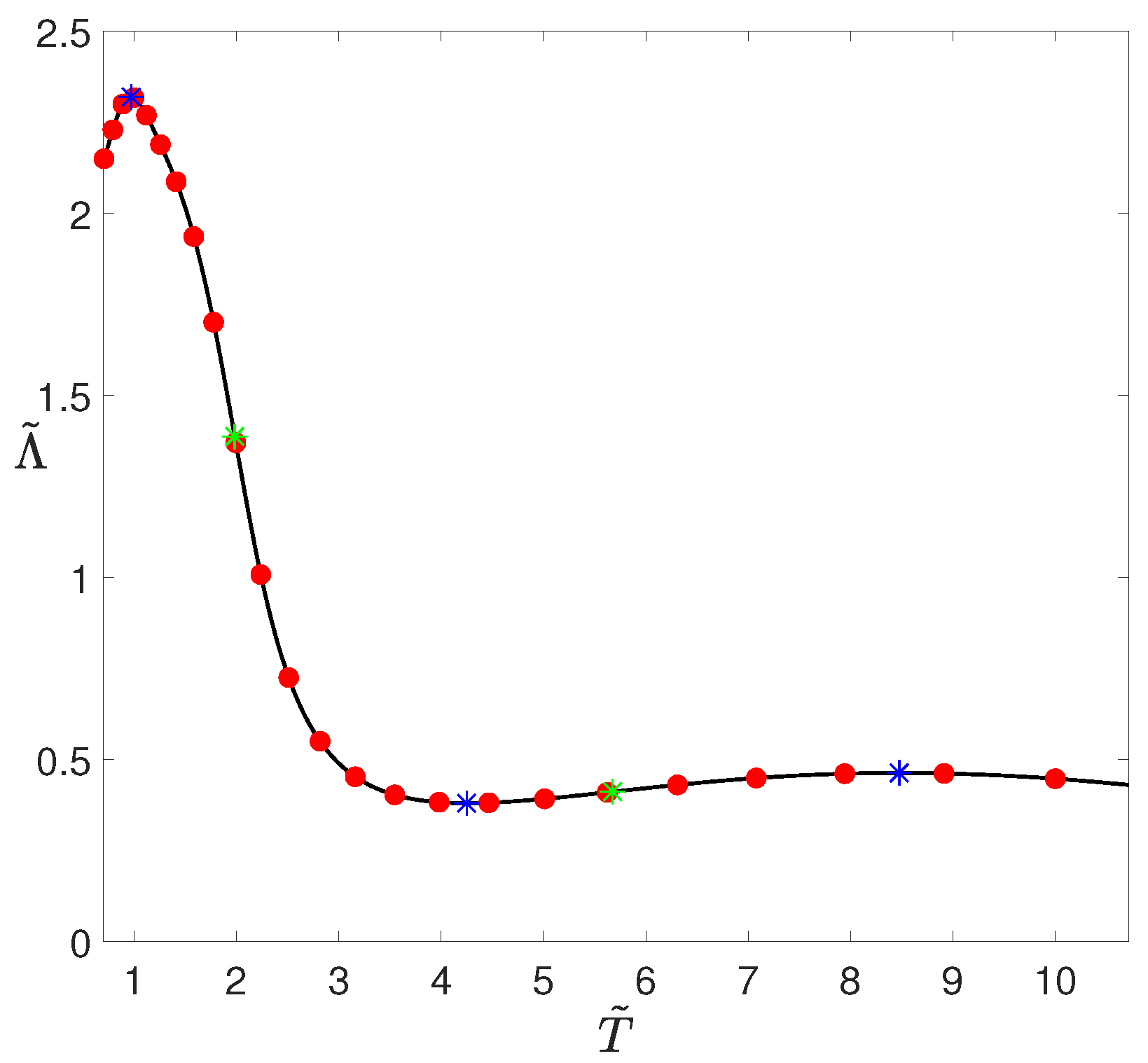
2.2. Interpolation of a Radiative-Loss Function

To obtain an analytical representation of the radiative-loss function, the cubic spline interpolation method was used. The interpolation for the temperature range from 1 to 10 MK was built for the points where wave phenomena were observed. This method allows us to express the radiative-loss function given by a number of values at some points. For each interval between adjacent points, a polynomial is constructed in such a way that the function and its derivatives are continuous up to a certain order on the boundary between adjacent intervals. These complete ones are called splines; for cubic splines, derivatives up to the second order inclusive are continuous. Thus, interpolation by cubic splines gives us an approximate analytical representation of the function Λ ( T ) with a continuous second derivative. The interpolation is based on the temperature range from 0.5 to 14.1 MK—that is, for all the temperatures of interest here. This allows us to obtain an approximate analytical expression around any point in this interval. Table 1 lists the values of the coronal plasma emission intensity at particle density n = 10 15 m 3 , obtained using the code CHIANTI 10 [32]. In what follows, the intensity is calculated in ergs.
The temperature values used, T i , i = 0, 1, 2,…, 28, are distributed in 29 intervals ( T i , T i + 1 ). A third-degree polynomial was constructed for each interval, so that at the ends of the interval, the polynomial takes the values of the function Λ ( T ) : Λ i Λ ( T i ) = D i and Λ i + 1 Λ ( T i + 1 ) = D i + 1 . This is convenient for finding the inflection points of a function where the second derivative vanishes. For the temperature and radiative-loss function, the scales m ( T ) = 10 6 K and m ( Λ ) = 10 26 erg · g 2 · cm 3 · s 1 are introduced, then their dimensionless values are:
T ˜ = m ( T ) 1 T , Λ ˜ = m ( Λ ) 1 Λ ,
so that the interpolation polynomials and the derivatives can be written in the form:
Λ ˜ = A ˜ i ( T ˜ T ˜ i ) 3 + B ˜ i ( T ˜ T ˜ i ) 2 + C ˜ i ( T ˜ T ˜ i ) + D ˜ i , Λ ˜ = 3 A ˜ i ( T ˜ T ˜ i ) 2 + 2 B ˜ i ( T ˜ T ˜ i ) + C ˜ i , i = 0 , 1 , , 28 .
Heareafter, the prime denotes the T ˜ -derivative and the tilde denotes dimensionless quantity. The values of the coefficients of the interpolation polynomials are given in Table 2. The interpolation is shown in Figure 2. The linear scale of values was chosen.

2.3. Basic Equations

Let us assume that the coronal plasma is an ideal gas, so that
p = ρ RT M ,
where R is the gas constant, M is the mean molar mass; M = μ N A , where μ is the average mass of a gas particle, and N A is the Avogadro constant. Further, we consider acoustic waves in an equilibrium medium with temperature T 0 and density ρ 0 ; ρ 0 = μ n 0 . Coronal loops where wave processes are observed are characterized by the value n 0 10 15 m 3 [8,9,33]. Let us define it as particle-density scale, m ( n ) = 10 15 m 3 . If define the mass density scale is defined as m ( ρ ) = 10 12 kg · m 3 , one gets the relation ρ ˜ 0 = 1.037 n ˜ 0 between dimensionless values of mass and particle densities.
We use the equations of one-dimensional gas dynamics for studying waves:
v x t + v x v x x = R M T x RT M ρ ρ x ,
ρ t + ( ρ v x ) x = 0 .
Here, x , v , and t denote the space coordinate, the gas velocity, and the time, respectively.
Let us write the energy balance equation in terms of temperature:
T t + v x T x + ( γ 1 ) T v x x = ( γ 1 ) M R Q ,
where Q (in J · kg 1 · s 1 ) denotes the amount of heat loss per unit time per unit mass of gas. Here, γ is an adiabatic index; γ = 5 / 3 here. In recent years, the study of the damping of acoustic waves in high-temperature coronal plasma has been carried out [13,14,15], while taking into account the effects of thermal conduction and heating/radiative loss:
Q = Q th + Q hc ,
Q th = 1 ρ x ϰ ( T ) T x .
We follow this approach in the present study and take the thermal conductivity as equal to
ϰ = 4.4 · 10 10 T 5 / 2 Λ C J m · s · K ,
according to Spitzer [34]. In this case, the Coulomb logarithm is Λ C = 19.3 for temperature T 1 MK and Λ C = 21.6 for T 10 MK and concentration n = 10 15 m 3 . Let us introduce the scale of the thermal conductivity, m ( ϰ ) = 10 4 J · m 1 · s 1 · K 1 , and its dimensionless value:
ϰ ˜ = 44 · T ˜ 5 / 2 / Λ C .
When T ˜ 1 MK and T ˜ 10 MK, one gets:
ϰ ˜ ( 1 ) = 2.28 · T ˜ 5 / 2 , ϰ ˜ ( 10 ) = 2.04 · T ˜ 5 / 2 ,
respectively.
Let us write linearized equations for linear waves in an equilibrium medium with the parameters ρ 0 and T 0 :
v x t = R M T x RT 0 M ρ 0 ρ x ,
ρ t + ρ 0 v x x = 0 ,
T t + ( γ 1 ) T 0 v x x = ( γ 1 ) M R ρ 0 ϰ ( T 0 ) 2 T x 2 ( γ 1 ) M R [ ρ 0 Λ ( T 0 ) T + ρ Λ ( T 0 ) ] .
The observed waves have a period about of 1 min or larger, which means that the oscillation frequency has values about of 0.1 s or smaller. Let us take the frequency scale equal to m ( ω ) = 0.1 s 1 . We use a dispersion relation for an adiabatic acoustic wave to obtain the wavenumber scale; that is, we assume m ( ω ) = m ( C s ) m ( k ) . For T 0 = 1 MK, the speed of sound is equal to 1.49 · 10 5 m · s 1 . Then, the speed of sound scale, m ( C s ) = 10 5 m · s 1 ; as a result, the scale of the wavenumber values is equal to m ( k ) = 10 6 m 1 .
The wave distributions will be considered as functions of dimensionless variables in the form exp ( i k ˜ x ˜ i ω ˜ t ˜ ) . Scales of spatial and temporal variables are taken from relations, m ( k ) m ( x ) = 1 and m ( ω ) m ( t ) = 1 , so m ( x ) = 10 6 m = 1 Mm and m ( t ) = 10 s . We take the dispersion relation as the basis for studying linear waves, from which we find the frequency, ω , at a given wavenumber. The dispersion relation derived from Equations (17)–(19) can be written as
ω ˜ 3 + iA ω ˜ 2 ω ˜ C ˜ s 2 k ˜ 2 + iB = 0 ,
A = A 1 k ˜ 2 + A 2 , B = 1 γ A 1 k ˜ 2 A 2 + A 3 C ˜ s 2 k ˜ 2 .
The coefficients A 1 , A 2 , and A 3 , included in the imaginary part of the relation and having a central place in the analysis of a non-adiabatic behavior of the wave, are determined by the following expressions:
S = ( γ 1 ) Mm ( ρ ) / ( Rm ( ω ) ) ,
A 1 = Sm ( ϰ ) m ( k ) 2 ϰ ˜ ( T ˜ 0 ) / ( m ( ρ ) 2 ρ ˜ 0 ) 5.01 ϰ ˜ ( T ˜ 0 ) / ρ ˜ 0 ,
A 2 = Sm ( Λ ) ρ ˜ 0 Λ ˜ ( T ˜ 0 ) / m ( T ) 5.01 · 10 3 ρ ˜ 0 Λ ˜ ( T ˜ 0 ) ,
A 3 = Sm ( Λ ) ρ ˜ 0 Λ ˜ ( T ˜ 0 ) / ( m ( T ) T ˜ 0 ) 5.01 · 10 3 ρ ˜ 0 Λ ˜ ( T ˜ 0 ) / T ˜ 0 .
The coefficient A 1 is determined by the thermal conductivity, the coefficient A 3 is determined by the radiative-loss function, and the coefficient A 2 is determined by the derivative of the radiative-loss function. The coefficient A 1 enters the equation along with the factor k 2 , which means that the role of thermal conductivity is small in the limit k 0 . From the analysis of the radiative-loss function, one knows that there is a temperature interval where the function decreases and the coefficient A 2 has negative values. In this interval, an impact of the coefficient A 2 will be opposite to an impact of the coefficient A 3 . If the A 3 leads damping of the wave, then A 2 will weaken this damping, and probably, instead of damping, there will be an increase in oscillation.
The coefficients A 1 , A 2 , A 3 depend on the equilibrium parameters, T ˜ 0 and ρ ˜ 0 , and one can write the dispersion relation solution as ω ˜ = ω ˜ ( k ˜ , T ˜ 0 , ρ ˜ 0 ) ; in other words, the frequency is a function not only of the wavenumber, but also of the thermodynamic parameters of the equilibrium medium.

3. Results

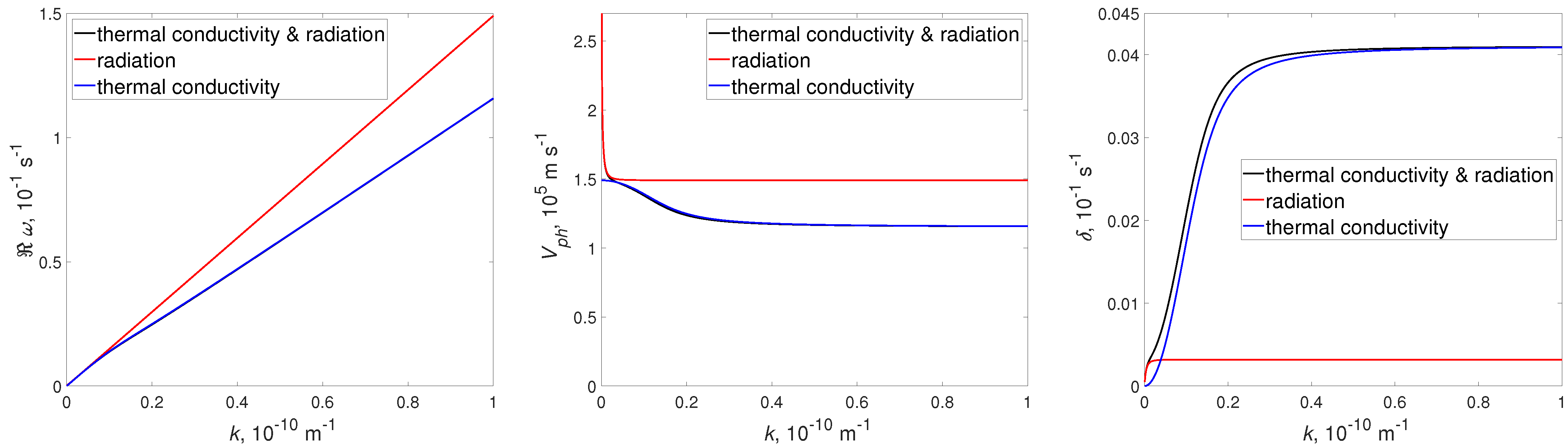
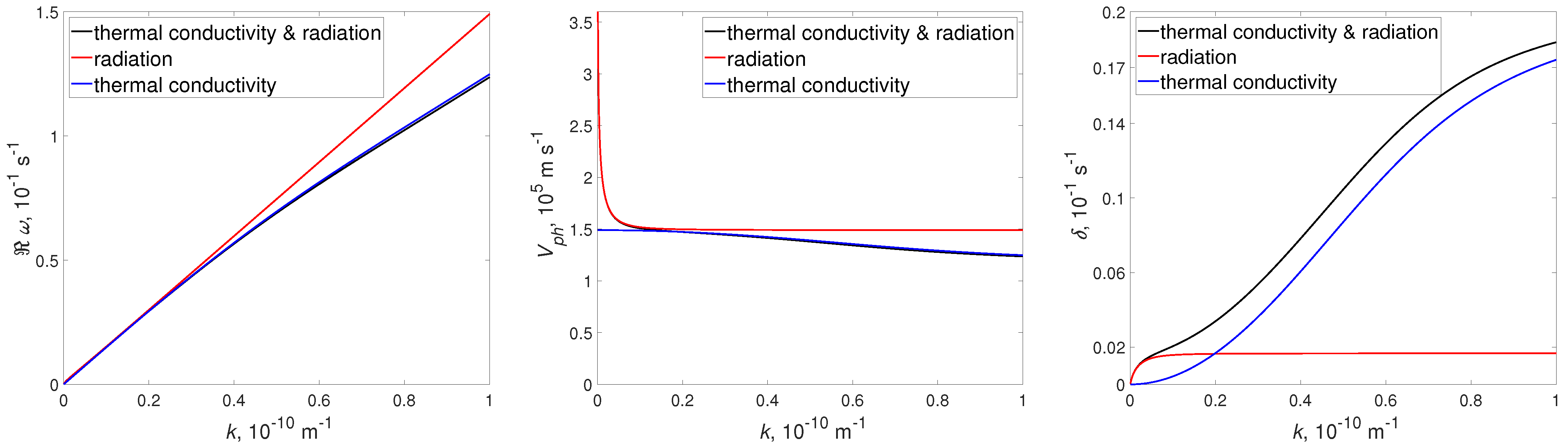
3.1. Wave Instability
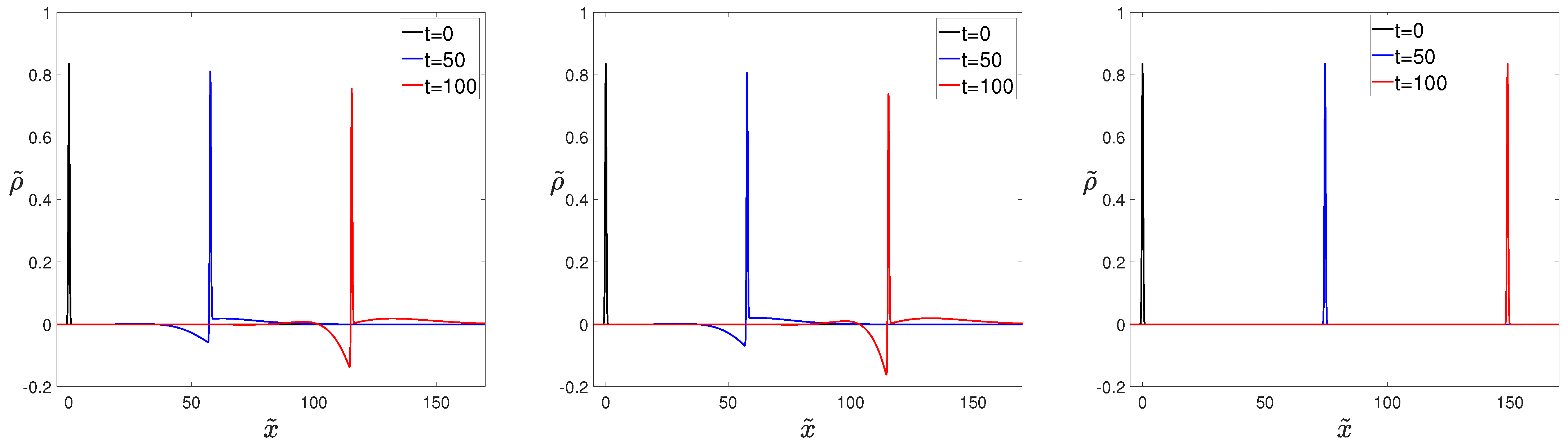
If the imaginary part of the frequency takes negative values, Im ω ˜ < 0 , then the oscillations are damped, and at Im ω ˜ > 0 , instability appears. Since frequency is a function of the wavenumber and thermodynamic parameters, the inequality Im ω ˜ ( k ˜ , T ˜ 0 , ρ ˜ 0 ) > 0 defines a domain of parameters, for which the acoustic wave is unstable. The equation Im ω ˜ ( k ˜ , T ˜ 0 , ρ ˜ 0 ) = 0 obviously determines the boundary of this domain. At the boundary, the dispersion relation can be written as
( Re ω ˜ ) 3 + i ( Re ω ˜ ) 2 ( A 1 k ˜ 2 + A 2 ) Re ω ˜ C ˜ s 2 k ˜ 2 i 1 γ A 1 C ˜ s 2 k ˜ 4 + i 1 γ ( A 3 A 2 ) C ˜ s 2 k ˜ 2 = 0 .
From the real part of the relation, one obtains the value Re ω ˜ = C s k ˜ and substitute it into the imaginary part:
( γ 1 ) A 1 k ˜ 2 + ( γ 1 ) A 2 + A 3 = 0 .
The stability exists when
( γ 1 ) A 1 k ˜ 2 + ( γ 1 ) A 2 + A 3 > 0 .
This inequality corresponds to the acoustic wave stability condition found by Field [20]. Since A 1 0 and A 3 0 , the appearance of instability is possible at ( γ 1 ) A 2 + A 3 ( γ 1 ) T ˜ 0 Λ ˜ ( T ˜ 0 ) + Λ ˜ ( T ˜ 0 ) < 0 , if the condition,
k ˜ < k ˜ c , k ˜ c = ( γ 1 ) A 2 + A 3 ( γ 1 ) A 1 ,
is met.
As the wavenumber increases, the influence of thermal conductivity increases, and when k ˜ > k ˜ c , an instability is stabilized by thermal conduction.
By writing the critical wavenumber as a function of the basic parameters,
k ˜ c ( ρ ˜ 0 , T ˜ 0 ) = ρ ˜ 0 F ( T ˜ 0 ) , F ( T ˜ 0 ) = ( γ 1 ) T ˜ 0 Λ ˜ ( T ˜ 0 ) + Λ ˜ ( T ˜ 0 ) ( γ 1 ) T ˜ 0 ϰ ˜ ( T ˜ 0 ) ,
one can find the boundary of the stability region in the parameter area ( k ˜ , T ˜ 0 , ρ ˜ 0 ) :
k ˜ = k ˜ c ( ρ ˜ 0 , T ˜ 0 ) .
The dimensionless values of the thermal conductivity, the radiative-loss function, and the derivative of the radiative-loss function are given in Table 3. From this Table, one can find the temperature values, at which the instability of the acoustic wave is possible; those temperature values are around T ˜ 0 2 . The derivative of the radiative-loss function has the largest negative value as an absolute value. For T ˜ 0 2.24 , one gets F ( T ˜ 0 ) 0.2 and k ˜ c 0.2 ρ ˜ 0 . Then, one can estimate the critical wavelength: λ ˜ c = 10 π / ρ ˜ 0 : λ ˜ c = 30.3 , λ c = 30.3 Mm for n ˜ 0 = 1 , i.e., n 0 = 10 15 m 3 . The instability appears at wavelengths exceeding the critical value. As the concentration of particles increases, the critical wavelength decreases, and at n 0 = 5 · 10 15 m 3 , the critical wavelength gets the value, λ c = 6.06 Mm .

3.2. Wave Damping

The acoustic oscillations are damped when Im ω ˜ < 0 , and the quantity δ = Im ω ˜ is the damping coefficient. We found the real and imaginary parts of the frequency and the phase velocity, V ph = Re ω / k , using the numerical solution of the dispersion relation (18) in the Maple 18 package. Figure 3 and Figure 4 show the corresponding dependence curves on the wavenumber in two special cases: T 0 = 10 6 K , n 0 = 1 · 10 15 m 3 and T 0 = 10 6 K , n 0 = 5 · 10 15 m 3 . In the future, we consider to perform a complete analysis of the behavior of the non-adiabatic waves based on the obtained interpolation of the radiative-loss function. Here, we show that the roles of thermal conductivity and heating/cooling in the wave damping may be ambiguous. In applications, one often ignores the role of heating/cooling in the damping of compression waves. As it is shown below, heating/cooling can make a noticeable contribution to the damping. In particular, a case when the effect of misbalance heating/cooling plays a dominant role in the wave damping is presented.
The asymptotic behavior of the frequency when k ˜ has the form ω ˜ v k i δ , with v = C ˜ s / γ , δ = ( γ 1 ) C ˜ s 2 / 2 γ A 1 . The limit value of the damping coefficient does not depend on k ˜ but depends on A 1 . At large wavenumbers, the damping weakens with an increase in A 1 , i.e., with an increase in the thermal conductivity. In the absence of thermal conductivity, the limit values of the phase speed and damping coefficient are equal to v = C ˜ s , δ = ( ( γ 1 ) A 2 + A 3 ) / 2 γ . The value ( γ 1 ) A 2 + A 3 is a certain parameter that characterizes a radiative damping. For example, when ( γ 1 ) A 2 + A 3 < 0 , stability of the acoustic oscillations may be lost.
From the damping coefficient curves k -dependence (Figure 3 and Figure 4), one can conclude that at large wavenumbers, the thermal conductivity dominates in the damping. The heating/radiative losses effect can compete only in the area of small wavenumbers. The boundary wavenumber separating the areas of influence of one and the other effect is equal to k ˜ = 0.04 in the case when n ˜ 0 = 1 and k ˜ = 0.2 , and when n ˜ 0 = 5 . The corresponding wavelengths are λ = 1.5 · 10 8 m and λ = 3 · 10 7 m , and the oscillation periods are about 600 s [1,4] and 200 s [2], respectively. These values are similar to the observed ones, which allows us to apply the theoretical model to the description of the observed events and estimate the plasma density from the parameters of the observed oscillations.

3.3. Wave Dispersion

The dispersion due to heating/radiative loss is effective only in a small range of small wavenumbers [35], and this area expands with increasing n 0 . For large k values, the dispersion is due to thermal conductivity. The cases considered here differ in the spectral localization of the dispersion: for n 0 = 1 · 10 15 m 3 , it is noticeable only in the intervals 0 < k ˜ < 0.4 and 0 < ω ˜ < 0.6 ; for n 0 = 5 · 10 15 m 3 , it goes into the area k ˜ > 1 and ω ˜ > 1.2 . The nature of the spectral localization of the dispersion affects the propagation of a group of waves. Here, this feature is shown with examples using modeling in Maple 18. Consider the initial localized Gaussian pulse,
ρ ˜ ( x ˜ , 0 ) = 1 6 0 e k ˜ 2 / 32 cos ( k ˜ x ˜ ) d k ˜ .
Here ρ ˜ is an unnormalized distribution describing the relative change in density. The degree of pulse localization in this example is high, its spatial extension is about m ( x ) = 1 Mm . For t ˜ > 0 , a behavior of a wave packet is determined by the Fourier’s cosine integral,
ρ ˜ ( x ˜ , t ˜ ) = 1 6 0 e k ˜ 2 / 32 cos ( k ˜ x ˜ ω ˜ t ˜ ) d k ˜ .
The integral (27) takes into account the dependence ω ˜ ( k ˜ ) obtained numerically from the dispersion relation (20). The simulation results are presented in Figure 5 and Figure 6.
In the second case ( n 0 = 5 · 10 15 m 3 ), shown in Figure 6, there is a decomposition of the initial pulse into separate components with different wavelengths. The observation of such perturbations in practice shows the presence of quasi-periodic oscillations of the plasma radiation intensity caused by a change in density. Knowing the periods can provide us with the information about the real dependence ω ( k ) and the physical parameters of the plasma. In the case when n 0 = 1 · 10 15 m 3 , the initial pulse during the first 1000 s (17 min) propagates practically without changing its shape. The propagation speed of the pulse is close to the speed of sound: C s = 1.49 · 10 5 m · s 1 . The dispersion is mainly due to the action of the thermal conductivity. From a comparison of Figure 5 and Figure 6, one can also conclude that the dispersion is more significant in the case of a dense plasma. One can consider this contradicting the remark made above that the effect of thermal conductivity weakens with increasing density. To resolve this contradiction, let us turn to the phase speed distributions. The phase speed of the wave under an influence of thermal conductivity changes within certain limits from C ˜ s at k ˜ = 0 to C ˜ s / γ for k ˜ . The area of wavenumbers, in which the conductivity charge varies is localized next to zero for large A 1 . As the density increases, the coefficient A 1 , which determines an influence of thermal conductivity, indeed decreases, but the area of this change in the phase speed expands, as can be seen from Figure 3 and Figure 4. The dispersion area affects large wavenumbers. This leads to the spreading of a narrow localized impulse, since the width of its Fourier transform in the area of large wavenumbers is quite large.

4. Discussion

When studying the mechanisms of the damping of acoustic waves in a highly-ionized, high-temperature plasma of the solar corona, preference is given to the effect of the thermal conduction [8,9]. At the same time, the role of radiative loss and possible sources of heating of the coronal plasma are noted. In particular, the misbalance of the heating/radiative loss leads to wave instability and dispersion [13,14,15]. The latter may be the cause of the generation of the quasi-periodic oscillations observed in the lower corona. Unlike thermal conductivity, the law of which is known for a strongly-ionized high-temperature plasma, the regularities of heating in various coronal regions are poorly understood. This circumstance strongly complicates the study of the non-adiabatic waves, and one often has to proceed from general ideas about how plasma heating can be described. In this case, a property of non-adiabaticity means that a possibility of energy exchange between individual parts of a plasma or between a plasma and an external medium. It is known that adiabatic waves are described by the energy balance equation (11) when the right-hand side equals zero. For non-adiabatic waves, the right-hand side of the equation is determined by the elementary processes of particle collision, radiation, and absorption of energy. To obtain these expressions, it is necessary to carry out an adequate procedure for closing kinetic equations for moments of the distribution functions. While these remain undefined, there are various approaches to this procedure, and of the most commonly used, Grad’s method can be noted. It should be noted that closure can lead to the appearance of additional relations for the thermodynamic parameters of plasma. This point requires further attentive study.
The calculation of the radiation intensity of the plasma of the solar atmosphere is possible and was carried out using the transfer equations and by taking into account all possible sources. There are various codes for this calculation, among which the CHIANTI [17,19,23] code is mostly used. This makes it possible to construct a radiative-loss function, which is done in this paper using the cubic interpolation method. Thus, in our opinion, we have obtained quite an adequate analytical description of radiative losses, which can be used in the study of acoustic waves. The sources of heating still remain unidentified in the phenomena under consideration, and we assume that heating has a stationary character. Actually, this means that the spatial and temporal scales of heating processes are large compared to the scales of wave phenomena.
An analysis of the dispersion relation showed that, over a significant interval of wavenumber values, thermal conductivity plays a decisive role in the damping and dispersion of the acoustic waves. The misbalance heating/cooling can compete with thermal conductivity only at low wavenumbers [35]. This statement was confirmed by the calculations here. The dispersion due to thermal conductivity extends over a wide area of the oscillation spectrum and can be the cause of the appearance of quasi-periodic oscillations with a wide frequency spectrum. On the contrary, the dispersion caused by the misbalance heating/cooling is localized in the area of low wavenumbers.
The specific form of the radiative-loss function obtained in this paper, makes it possible to find the conditions, under which the acoustic wave becomes unstable. Earlier, some abstract assumptions about the form of the heating/cooling function [13] were used for this. Its is shown here that instability is possible for certain wavelengths at temperatures where the radiative-loss function decreases. These findings are consistent with Field’s theoretical results [20].
The definiteness of the form of the radiative-loss function provides us with a model of the acoustic oscillations that can be used to diagnose coronal plasma. We built here a simple model of non-adiabatic acoustic waves and set a constant heating function. The main parameters in this model are the temperature and density of the coronal plasma, which can be determined from the parameters of the acoustic wave. In addition, a simple model of observed damped compression waves is built here for coronal seismology. The calculations made show that the obtained results agree with the observational data [1,2,4]. A more detailed and extended analysis of the acoustic oscillations using this model is beyond the scope of this paper. The constructed model can be changed by setting the heating function as a non-constant later, just as in coronal seismology, then the model of a magnetic tube to be modified with the heterogeneity introduced.

Author Contributions

Conceptualization, B.M.; methodology, B.M.; software, N.S.; validation, D.B.; formal analysis, D.B.; data curation, D.B.; writing—original draft preparation, S.D.; writing—review and editing, S.D.; funding acquisition, S.D. All authors have read and agreed to the published version of the manuscript.

Funding

This research was funded by Ministry of Science and Higher Education of the Russian Federation, grant number 075-03-2022-119/1.

Data Availability Statement

The CHIANTI data and code are available in Ref. [32].

Acknowledgments

The authors thank the referees for useful comments.

Conflicts of Interest

The authors declare no conflict of interest.

References

  1. Srivastava, A.K.; Kuridze, D.; Zaqarashvili, T.V.; Dwivedi, B.N. Intensity oscillations observed with Hinode near the south pole of the Sun: Leakage of low frequency magneto-acoustic waves into the solar corona. Astron. Astrophys. 2008, 481, L95–L98. [Google Scholar] [CrossRef]
  2. De Moortel, I. Longitudinal waves in coronal loops. Space Sci. Rev. 2009, 149, 65–81. [Google Scholar] [CrossRef]
  3. Banerjee, D.; Gupta, G.R.; Teriaca, L. Propagating MHD waves in coronal holes. Space Sci. Rev. 2011, 158, 267–288. [Google Scholar] [CrossRef]
  4. Banerjee, D.; Krishna Prasad, S. MHD waves in coronal holes. In Low-Frequency Waves in Space Plasmas; Keiling, A., Lee, D.-H., Nakariakov, V.M., Eds.; John Wiley & Sons, Inc.: New York, NY, USA, 2016; pp. 419–430. [Google Scholar] [CrossRef] [Green Version]
  5. Krishna Prasad, S.; Van Doorsselaere, T. Compressive oscillations in hot coronal loops: Are sloshing oscillations and standing slow waves independent? Astrophys. J. 2021, 914, 81. [Google Scholar] [CrossRef]
  6. Wang, T.J. Standing slow-mode waves in hot coronal loops: Observations, modeling, and coronal seismology. Space Sci. Rev. 2011, 158, 397–419. [Google Scholar] [CrossRef] [Green Version]
  7. De Moortel, I.; Nakariakov, V.M. Magnetohydrodynamic waves and coronal seismology: An overview of recent results. Phil. Trans. Roy. Soc. A 2012, 370, 3193–3216. [Google Scholar] [CrossRef] [Green Version]
  8. Ofman, L.; Wang, T. Hot coronal loop oscillations observed by SUMER: Slow magnetosonic wave damping by thermal conduction. Astrophys. J. 2002, 580, L85–L88. [Google Scholar] [CrossRef]
  9. De Moortel, I.; Hood, A.W. The damping of slow MHD waves in solar coronal magnetic fields. Astron. Astrophys. 2003, 408, 755–765. [Google Scholar] [CrossRef]
  10. Priest, E.R.; Foley, C.R.; Heyvaerts, J.; Arber, T.D.; Culhane, J.L.; Acton, L.W. Nature of the heating mechanism for the diffuse solar corona. Nature 1998, 393, 545–547. [Google Scholar] [CrossRef]
  11. Aschwanden, M.J.; Terradas, J. The effect of radiative cooling on coronal loop oscillations. Astrophys. J. 2008, 686, L127–L130. [Google Scholar] [CrossRef]
  12. Mikhalyaev, B.B.; Veselovskii, I.S.; Khongorova, O.V. Radiation effects on the MHD wave behavior in the solar corona. Sol. Syst. Res. 2013, 47, 50–57. [Google Scholar] [CrossRef]
  13. Kolotkov, D.Y.; Nakariakov, V.M.; Zavershinskii, D.I. Damping of slow magnetoacoustic oscillations by the misbalance between heating and cooling processes in the solar corona. Astron. Astrophys. 2019, 628, A133. [Google Scholar] [CrossRef] [Green Version]
  14. Zavershinskii, D.I.; Kolotkov, D.Y.; Nakariakov, V.M.; Molevich, N.E.; Ryashchikov, D.S. Formation of quasi-periodic slow magnetoacoustic wave trains by the heating/cooling misbalance. Phys. Plasmas 2019, 26, 082113. [Google Scholar] [CrossRef] [Green Version]
  15. Belov, S.A.; Molevich, N.E.; Zavershinskii, D.L. Dispersion of slow magnetoacoustic waves in the active region fan loops introduced by thermal misbalance. Sol. Phys. 2021, 296, 122. [Google Scholar] [CrossRef]
  16. Ginzburg, V.L. Concerning the general relationship between absorption and dispersion of sound waves. Sov. Phys. - Acoustics 1955, 1, 32–41. [Google Scholar]
  17. Dere, K.P.; Landi, E.; Young, P.R.; Del Zanna, G.; Landini, M.; Mason, H.E. CHIANTI—An atomic database for emission lines IX. Ionization rates, recombination rates, ionization equilibria for the elements hydrogen through zinc and updated atomic data. Astron. Astrophys. 2009, 498, 915–929. [Google Scholar] [CrossRef]
  18. Dudík, J.; Dzifčáková, E.; Karlický, M.; Kulinová, A. The bound-bound and free-free radiative losses for the nonthermal distributions in solar and stellar coronae. Astron. Astrophys. 2011, 529, A103. [Google Scholar] [CrossRef]
  19. Del Zanna, G.; Dere, K.P.; Young, P.R.; Landi, E. CHIANTI—An atomic database for emission lines. XVI. Version 10, further extensions. Astrophys. J. 2021, 909, 38. [Google Scholar] [CrossRef]
  20. Field, G.B. Thermal instability. Astrophys. J. 1965, 142, 531–567. [Google Scholar] [CrossRef]
  21. Priest, E.R. Magnetohydrodynamics of the Sun; Cambridge University Press: Cambridge, UK, 2014. [Google Scholar] [CrossRef]
  22. Dere, K.P.; Landi, E.; Mason, H.E.; Monsignori Fossi, B.C.; Young, P.R. CHIANTI—An atomic database for emission lines. I. Wavelengths greater than 50 Å. Astron. Astrophys. Suppl. Ser. 1997, 125, 149–173. [Google Scholar] [CrossRef] [Green Version]
  23. Landi, E.; Landini, M. Radiative losses of optically thin coronal plasmas. Astron. Astrophys. 1999, 347, 401–408. Available online: https://ui.adsabs.harvard.edu/abs/1999A%26A...347..401L/ (accessed on 25 January 2023).
  24. Rosner, R.; Tucker, W.H.; Vaiana, G.S. Dynamics of the quiescent solar corona. Astrophys. J. 1978, 220, 643–665. [Google Scholar] [CrossRef]
  25. Carbonell, M.; Oliver, R.; Ballester, J.L. Time damping of linear non-adiabatic magnetohydrodynamic waves in an unbounded plasma with solar coronal properties. Astron. Astrophys. 2004, 45, 739–750. [Google Scholar] [CrossRef] [Green Version]
  26. Klimchuk, J.A.; Patsourakos, S.; Cargill, P.J. Highly efficient modeling of dynamic coronal loops. Astrophys. J. 2008, 682, 1351–1362. [Google Scholar] [CrossRef] [Green Version]
  27. Landi, E.; Del Zanna, G.; Young, P.R.; Dere, K.P.; Mason, H.E.; Landini, M. CHIANTI—An atomic database for emission lines. VII. New data for X-rays and other improvements. Astrophys. J. Supp. Ser. 2006, 162, 261–280. [Google Scholar] [CrossRef] [Green Version]
  28. Parker, E.N. Instability of thermal fields. Astrophys. J. 1953, 117, 431–436. [Google Scholar] [CrossRef]
  29. Weymann, R. Heating of stellar chromospheres by shock waves. Astrophys. J. 1960, 132, 452–460. [Google Scholar] [CrossRef]
  30. Kolotkov, D.Y.; Duckenfield, T.J.; Nakariakov, V.M. Seismological constraints on the solar coronal heating function. Astron. Astrophys. 2020, 644, A33. [Google Scholar] [CrossRef]
  31. Kolotkov, D.Y.; Zavershinskii, D.I.; Nakariakov, V.M. The solar corona as an active medium for magnetoacoustic waves. Plasma Phys. Control. Fusion 2021, 63, 124008. [Google Scholar] [CrossRef]
  32. CHIANTI: An Atomic Database for Spectroscopic Diagnostics of Astrophysical Plasmas. Available online: http://www.chiantidatabase.org (accessed on 25 January 2023).
  33. Reale, F. Coronal loops: Observations and modeling of onfined plasma. Living Rev. Sol. Phys. 2014, 11, 4. [Google Scholar] [CrossRef]
  34. Spitzer, L., Jr. Physics of Fully Ionized Gases; Dover Publications, Inc.: Mineola, NY, USA, 2006. [Google Scholar]
  35. Nakariakov, V.M.; Afanasyev, A.N.; Kumar, S.; Moon, Y.-J. Effect of local thermal equilibrium misbalance on long-wavelength slow magnetoacoustic waves. Astrophys. J. 2017, 849, 62. [Google Scholar] [CrossRef]
Figure 1. Radiative-loss function as given by CHIANTI v5.2 earlier studies [27]. Adopted from Ref. [18].
Physics 05 00017 g001
Figure 2. Interpolation curve (7) of the radiative-loss function for temperatures 1 to 10 MK. The red dots represent the radiative-loss function values from Table 1. The asterisks indicate the extremum and inflection points.
Physics 05 00017 g002
Figure 3. The frequency real part (left), the phase speed, V ph = ω / k (middle) and the damping coefficient, δ = Im ω ˜ (right) for T 0 = 10 6 K , n 0 = 1 · 10 15 m 3 . See text for more details.
Physics 05 00017 g003
Figure 4. The frequency real part (left), the phase speed, V ph = ω / k (middle) and the damping coefficient, δ = Im ω ˜ (right) for T 0 = 10 6 K , n 0 = 5 · 10 15 m 3 . See text for more details.
Physics 05 00017 g004
Figure 5. Localized pulse dispersion due to thermal conductivity and heating/cooling (left), thermal conductivity only (middle), and heating/cooling only (right) for T 0 = 10 6 K , n 0 = 1 · 10 15 m 3 .
Physics 05 00017 g005
Figure 6. Localized pulse dispersion due to thermal conductivity and heating/cooling (left), thermal conductivity only (middle), and heating/cooling only (right) for T 0 = 10 6 K , n 0 = 5 · 10 15 m 3 .
Physics 05 00017 g006
Table 1. The values of the radiative-loss function Λ i , as a function of temperature, T i . ρ and n denote the plasma and particle densities, respectively.
i T i (K),  × 10 6 ρ 2 Λ i / n 2 ( erg · cm 3 · s 1 ) × 10 22 Λ i ( erg · g 2 · cm 3 · s 1 ) × 10 26
00.50118722.2678292.108884
10.5623412.3674342.201509
20.6309572.4181562.248675
30.7079462.4691512.296096
40.7943282.5479262.369351
50.8912512.6228822.439053
612.6462712.460803
71.1220182.6023112.419923
81.2589252.5235372.346671
91.4125382.4216562.25193
101.5848932.2665812.107724
111.7782792.0196011.878054
121.9952621.6653441.548626
132.2387211.2690711.180126
142.5118860.9465410.880201
152.8183830.7298570.678704
163.1622780.595830.55407
173.5481340.520040.483592
183.9810720.4830170.449164
194.4668360.4711060.438087
205.0118720.4748390.441559
215.6234130.4874750.45331
226.3095730.5041560.468822
237.0794580.5204850.484006
247.9432820.5311250.493901
258.9125090.5303890.493216
26100.5131760.47721
2711.2201850.4764650.443071
2812.5892540.4212380.391715
2914.1253750.3579610.332873
Table 2. Coefficients of the dimensionless cubic interpolation (7).
iAiBiCiDi
0−8.164325−6.6550461.9521252.108884
142.533874−8.1528921.0465592.201509
26.9279440.6026240.528492.248675
3−11.6222742.2027380.744472.296096
4−7.161141-0.8091430.8648532.36935
50.696996−2.8913750.5061892.439053
65.9093052−2.6639816−0.0979512.4608027
70.940888−0.500849−0.4841192.419923
8−1.306459−0.114406−0.5683522.3466709
9−0.579185−0.71647−0.6959852.25193
100.091538−1.015948−0.9945772.107724
111.443157−0.962841−1.3772471.878054
121.4062024−0.02342−1.5912491.548626
13−0.2615021.003637−1.3526061.180126
14−0.3888050.789338−0.8628280.880201
15−0.1892460.431835−0.4885430.678704
16−0.1025620.236593−0.2586740.55407
17−0.0461610.117871−0.1219020.483592
18−0.0217790.057916−0.0457970.449164
19−0.0099370.026178−0.0049470.438087
20−0.0042510.0099290.01473250.044156
21−0.0020430.0021310.02210720.453309
22−0.001395−0.207380.0221460.468822
23−0.000595−0.0052960.01647280.484006
24−0.000074−0.0068390.0059910.4939
250.000361−0.007054−0.0074740.493216
260.00049−0.005878−0.0215360.47721
270.000944−0.004084−0.0336910.443071
280.000667−0.000021−0.0395630.391715
Table 3. The values of the dimensionless thermal conductivity, ϰ ˜ , the radiative-loss function, Λ ˜ , and the its derivative, Λ ˜ . γ = 5 / 3 is the adiabatic index.
i T ˜ i ϰ ˜ ( T ˜ i ) Λ ˜ ( T ˜ i ) Λ ˜ ( T ˜ i ) / T ˜ i ( γ 1 ) Λ ˜ ( T ˜ i ) + Λ ˜ ( T ˜ i ) / T ˜ i
00.5011870.4054481.9521254.2077785.509194
10.5623410.5406731.046563.91494.6126
20.630960.7210.528493.56393.916237
30.7079460.9614680.7444713.2433223.739636
40.7943281.2821380.8648532.9828363.559404
50.8912511.7097590.5061892.7366633.074122
612.28−0.0979512.4608032.395502
71.1220193.040429−0.4841192.1567591.834013
81.2589254.054477−0.5683521.8640271.485126
91.4125385.406732−0.6959851.5942441.130255
101.5848937.209993−0.9945771.3298840.666833
111.7782799.61468−1.3772471.0561070.137943
121.99526212.821382−1.5912490.776152−0.284681
132.23872117.097588−1.3526060.527143−0.374595
142.511886422.8−0.8628280.350415−0.224804
152.81838330.404289−0.4885430.240813−0.084882
163.16227840.544771−0.2586740.1752120.002763
173.54813454.06732−0.1219020.1362950.055027
183.98107272.099931−0.0457970.1128250.008229
194.46683696.146803−0.0049470.0980760.094778
205.011872128.213820.0147330.0881030.097924
215.623413170.975880.0221070.0806110.095349
226.3095732280.0221460.0743030.089068
237.079458304.042890.0164730.0683680.07935
247.943282405.447710.0059910.0621780.066172
258.912509540.6732−0.0074740.055340.050357
2610720.9993−0.0215360.0477210.033363
2711.220185961.46803−0.0336910.0394890.017028
2812.5892541 282.1382−0.0395630.0311150.00474
Disclaimer/Publisher’s Note: The statements, opinions and data contained in all publications are solely those of the individual author(s) and contributor(s) and not of MDPI and/or the editor(s). MDPI and/or the editor(s) disclaim responsibility for any injury to people or property resulting from any ideas, methods, instructions or products referred to in the content.

