Polygon-Based Hierarchical Planar Networks Based on Generalized Apollonian Construction

Abstract

Experimentally observed complex networks are often scale-free, small-world and have an unexpectedly large number of small cycles. An Apollonian network is one notable example of a model network simultaneously having all three of these properties. This network is constructed by a deterministic procedure of consequentially splitting a triangle into smaller and smaller triangles. In this paper, a similar construction based on the consequential splitting of tetragons and other polygons with an even number of edges is presented. The suggested procedure is stochastic and results in the ensemble of planar scale-free graphs. In the limit of a large number of splittings, the degree distribution of the graph converges to a true power law with an exponent, which is smaller than three in the case of tetragons and larger than three for polygons with a larger number of edges. It is shown that it is possible to stochastically mix tetragon-based and hexagon-based constructions to obtain an ensemble of graphs with a tunable exponent of degree distribution. Other possible planar generalizations of the Apollonian procedure are also briefly discussed.

1. Introduction

It is often convenient to present big volumes of data as a graph, i.e., as a set of objects and binary relations (bonds) between them. This approach naturally arises in numerous contexts ranging from physics of disordered systems [1] and biology [2] to sociology [3] and linguistics (see, e.g., [4,5,6]). The rapid growth in information technology ensures that larger and larger datasets of this type are becoming available. This naturally stimulates interest in the tools to analyze these datasets and simple (or not so simple) reference mathematical models, which can be used to probe their properties. Thus, a rapid development in the last 20 years of a new interdisciplinary field on the boundary of the random graph theory, the data analysis and the statistical physics, known as complex network theory [7,8,9], has occurred.

Among the structural characteristics typical for many experimentally observed networks, there are three especially common and striking (see, e.g., [7]): (i) the small-world property (a very small average node-to-node distance measured along the network), (ii) extremely wide, approximately a power-law distribution of the node degrees (the networks with this property are often called ‘scale-free’), and (iii) large, as compared to referent randomized networks, the concentration of the short circles (e.g., triangles). It is reasonably easy to construct a model network that has one or two of these characteristics, e.g., Erdos–Rényi graphs [10,11] are small-world, random geometrical graphs [12] that have a large clustering coefficient. The Barabási–Albert model [13] generates small-world scale-free networks. The Watts–Strogatts model [14] generates small-world graphs with a large clustering coefficient, etc. Generating all three properties simultaneously is much harder. Random geometric networks in a hyperbolic space [15,16,17] constitute one example of networks with these properties. Another one is the Apollonian network.

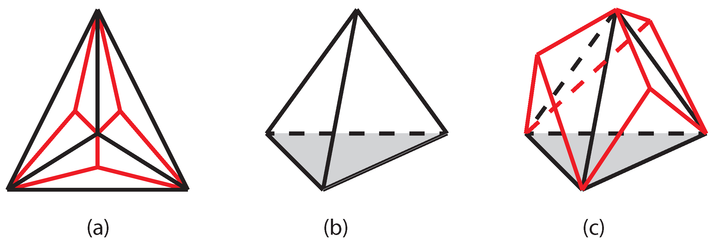
The Apollonian network [18,19] is a planar graph that arises naturally as a network representation of the Apollonian gasket, a remarkable object, which is, apparently, the first known fractal (interestingly, its exact fractal dimension is still unknown) [20,21]. The construction of this network can be explained recursively as follows; see Figure 1. Take a triangle, pick a point inside it and connect it to the three corners of the triangle. As a result, one obtains a set of 3 adjacent triangles that form the first-generation Apollonian network. Now, pick a point inside each of the three triangles, and connect it to its corners, this gives a second-generation Apollonian network, then repeat ad infinitum. The resulting network has been studied extensively in recent years, and it has been shown to have many beautiful properties. For example, the degree distribution and the clustering coefficient have been calculated [18], as well as the average path length [22]. Notably, there is an interesting non-planar interpretation of the Apollonian network. Namely, it can be thought of as a simplicial complex in the following way [23]. A first-generation Apollonian network is a tetrahedron (3-simplex). A second-generation Apollonian network consists of four tetrahedra: the original one and another three, each having a common two-face with the original one. A third-generation Apollonian network consists of 13 tetrahedra: one produced in the first generation, three produced in the second generation and nine new ones attached to each free face of the three second-generation tetrahedra, etc. Thus, one can think of an Apollonian network as a regular rooted tree of tetrahedra touching each other by common faces. This construction is easy to visualize in a 3-dimensional (3D) space (see Figure 1b,c), and it makes the Apollonian network a natural discretization of the 3D hyperbolic space in the same way as a regular tree is a natural discretization of the hyperbolic plane. Many properties of the Apollonian network can be calculated exactly, which makes it a nice toy model for the study of various properties of real scale-free networks. As a result, there have been a significant number of papers in recent years studying percolation [23], spin models [24], signal spreading [25], synchronization [26], traffic [27], random walks [28,29], etc., on the Apollonian network.

Despite being such a beautiful and well-studied object, the Apollonian network has certain drawbacks as a model of real networks. Most importantly, it is a single deterministic object with certain fixed properties, e.g., a fixed degree distribution with a fixed power law exponent $\gamma =ln3/ln2$. Importantly, that degree distribution is not a true power law but rather a log-periodic distribution consisting of a sequence of atoms at points $3\times 2^n$ and a power-law envelope. This means that the network is scale-invariant only with respect to certain discrete renormalizations and thus do not have the full set of properties of a true power law distribution; see [30] for a recent discussion. One natural generalization is a random Apollonian network [31,32,33], which is constructed, instead of a regular generation-by-generation process, by sequential partitioning of arbitrarily chosen triangles. The average degree distribution in such network is a true power law with exponent ${\gamma }_R=3$ [32]. Notably, to the best of our knowledge, random Apollonian graphs remain the only scale-free planar graph model with a continuously growing size for which the exact degree distribution exponent is known. Another way of generalizing the network is to consider the k-simpliceswith $k>3$ as building blocks of the network construction procedure. This gives rise to multidimensional Apollonian networks [34,35].

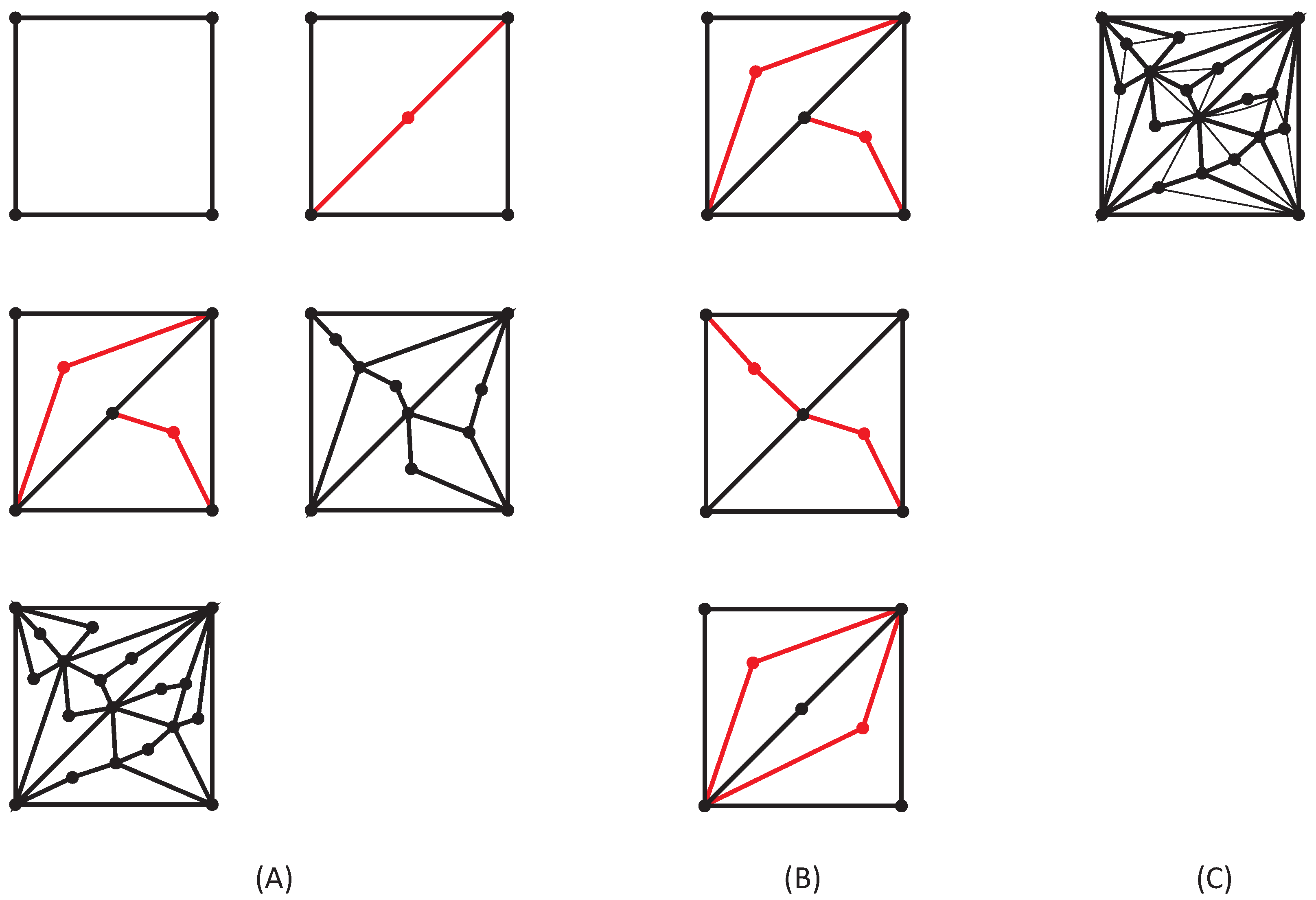
In this paper, the authors suggest another way of generalizing the Apollonian network construction. As a result, a novel famility of small-world, scale-free planar networks is obtained. The main idea is to construct an Apollonian-style iteration procedure based on polygons with different numbers of edges. The paper is organized as follows. In Section 2, a tetragon-based Apollonian-style network is constructed and the corresponding degree distribution is explicitely calculated. Then, the suggested procedure is generalized to polygons with an arbitrary even number of edges. In Section 4, it is shown that it is possible to construct a continuous one-parametric family of models interpolating between the tetragon- and hexagon-based models and demonstrate that the models in this family have a power low degree distribution with an exponent depending on the parameter, so it is possible to adjust it to fit the desired degree distribution (note that the adjustable exponent of the degree distribution can be obtained by different means in the so-called Evolving Apollonian networks [26,33]). Last section, summarizes the results of the paper and discusses further open questions and possible generalizations.

2. Tetragon-Based Network

2.1. Definition

Among several possible ways of generalizing the procedure described above to the case of polygons, consider the following procedure defined here for tetragons but easy to generalize for any polygon with an even number of edges. Note that given that we make such a generalization in further sections, we prefer to use the term ‘tetragon’ rather than ‘quadrilateral’ for a polygon with 4 sides in order to make the terminology more uniform.

Take a tetragon and pick a point inside it; then choose (at random) a pair of non-adjacent vertices of the original tetragon and connect them with a polyline with one new intermediate point. One now has two adjacent tetragons, for which one can repeat this construction, as shown in Figure 2. Importantly, contrary to the standard Apollonian network, which is a deterministic object, the network resulting from this procedure is stochastic. Indeed, already in the second generation, there are three topologically different realizations of the network, see Figure 2B. Notably, at any generation, this network has no triangles and is, in fact, bipartite.

2.2. Degree Distribution

The natural question to ask about this newly introduced class of planar Apollonian-like networks is what is the degree distribution of the nodes $G_n\left(k\right)$ in the n-th generation of the network and what distribution $\mathcal{G}\left(k\right)$ it converges to for $n\to \infty$ (here and in what follows the term “degree distribution” is used to mean the probability density function, i.e., the probability for the node to have a degree equal to k, as opposed to the cumulative distribution function, i.e., the probability for the node to have a degree larger or equal to k). By analogy with the Apollonian networks, one expects $\mathcal{G}\left(k\right)$ to be scale-free, i.e.,

$$\mathcal{G}\left(k\right)\simeq C{k}^{-\alpha },k\gg 1,$$

(1)

with some yet unknown constants C and $\alpha$.

To calculate the degree distribution $G_n\left(k\right)$, note that the degree of any given node is a random variable, whose distribution $F_{n-m}\left(k\right)$ for all nodes except the four initial ones depends only on the number of generations between the generation m at which it was created and current generation n. Indeed, each node with degree k has exactly k adjacent tetragons ($k-1$ for the four initial nodes), and at every step of the recurrent procedure, each of these tetragons is split in two, which results in the creation of a new edge adjacent to the node with the probability 1/2 (in the other half of the cases, the splitting path does not go through the given node). These splitting events happen independently for all tetragons. The overall degree distribution is therefore calculated by averaging over degree distributions of different generations:

$$G_n^{\mathrm{all}}\left(k\right)={\displaystyle \frac{4F_n^{\left(0\right)}\left(k\right)+{\sum }_{m=1}^n{Q}_m{F}_{n-m}\left(k\right)}{4+{\sum }_{m=1}^n{Q}_m}}=\frac{4}{2^n+3}{F}_n^{\left(0\right)}\left(k\right)+\frac{2^n-1}{2^n+3}{G}_n\left(k\right),G_n\left(k\right)=\frac{{\sum }_{m=1}^n{Q}_m{F}_{n-m}\left(k\right)}{{\sum }_{m=1}^n{Q}_m},$$

(2)

where $Q_m=2^{m-1}$ is the number of nodes created in the m-th generation, $F_n^{\left(0\right)}\left(k\right)$ is the degree distribution of the four initial nodes, and it is convenient to introduce $G_n\left(k\right)$, the degree distribution of all nodes except four initial ones.

2.3. Recurrence Relation for $F_n\left(K\right)$

To construct the recurrence relation for $F_n\left(k\right)$ proceed as follows. Let l be the degree of a node in the $(n-1)$-th generation. This means that this node has l tetragons adjacent to it, and when constructing the n-th generation of the network, each of them will be split in half, and with probability 1/2, the splitting path will go through the node under consideration. Every such path increases the degree of the node by one. Thus, the overall degree may increase by $l^{\prime }$, $0\le l^{\prime }\le l$, with the probability $2^{-l}\left(\genfrac{}{}{0pt}{}{l}{l^{\prime }}\right)$, leading to

$$F_n\left(k\right)=\sum _{l=\lfloor (k+1)/2\rfloor }^k{2}^{-l}\left(\genfrac{}{}{0pt}{}{l}{k-l}\right)F_{n-1}\left(l\right)\mathrm{for}n\ge 1,F_0\left(k\right)={\delta }_{k,2},$$

(3)

where the fact that all nodes are created with degree 2 is taken into account and the notation $\lfloor x\rfloor$ is introduced for the integer part of x (i.e., greatest integer less or equal to x). This equation can be written down in a simpler form in terms of a generating function,

$$f_n\left(\lambda \right)=\sum _{k=2}^{\infty }{\lambda }^k{F}_n\left(k\right).$$

(4)

Indeed, after substituting Equation (3), one obtains $f_0\left(\lambda \right)={\lambda }^2$ and

$$\begin{array}{ccc}\hfill f_n\left(\lambda \right)& =\hfill & {\displaystyle \sum _{k=2}^{\infty }\sum _{l=\lfloor (k+1)/2\rfloor }^k{\lambda }^k{2}^{-l}\left(\genfrac{}{}{0pt}{}{l}{k-l}\right)F_{n-1}\left(l\right)}\hfill \\ \hfill & =\hfill & {\displaystyle \sum _{l=2}^{\infty }\sum _{m=0}^l{(\lambda /2)}^l\left(\genfrac{}{}{0pt}{}{l}{m}\right){\lambda }^m{F}_{n-1}\left(l\right)=\sum _{l=2}^{\infty }{\left(\frac{\lambda (1+\lambda )}{2}\right)}^l{F}_{n-1}\left(l\right)=f_{n-1}\left(\frac{\lambda (1+\lambda )}{2}\right),}\hfill \end{array}$$

(5)

where the order of summation is changed, $m=k-l$ is introduced, and the binomial formula,

$${(1+\lambda )}^l=\sum _{m=0}^l\left(\genfrac{}{}{0pt}{}{l}{m}\right){\lambda }^m,$$

(6)

is used. The recurrence relation for the four initial nodes is a bit different because in their case, the node of degree l has only $l-1$ adjacent tetragons:

$$F_n^{\left(0\right)}\left(k\right)=\sum _{l=\lfloor k/2\rfloor +1}^k{2}^{-l+1}\left(\genfrac{}{}{0pt}{}{l-1}{k-l+1}\right)F_{n-1}^{\left(0\right)}\left(l\right)\mathrm{for}n\ge 1,F_0\left(k\right)={\delta }_{k,2},$$

(7)

which leads to the following equation for the generating function

$$f_n^{\left(0\right)}\left(\lambda \right)=\sum _{k=2}^{\infty }{\lambda }^k{F}_n^{\left(0\right)}\left(k\right)=\frac{2}{1+\lambda }{f}_{n-1}^{\left(0\right)}\left(\frac{\lambda (1+\lambda )}{2}\right),$$

(8)

In the $n\to \infty$ limit, both $f_n\left(\lambda \right)$ and $f_n^{\left(0\right)}\left(\lambda \right)$ converge to zero for all $\left|\lambda \right|<1$. Indeed, the probability to have any finite degree many generations after the creation of a node is exponentially small.

2.4. Generating Function of the Degree Distribution

Combining Equation (2) for $G_n\left(k\right),G_n^{\mathrm{all}}\left(k\right)$ and the equations for the generating functions (5) and (8), one gets the recurrence relation for the full degree distributions in terms of generating functions:

$$g_n\left(\lambda \right)=\sum _k{G}_n\left(k\right){\lambda }^k,g_n^{\mathrm{all}}\left(\lambda \right)=\sum _k{G}_n^{\mathrm{all}}\left(k\right){\lambda }^k.$$

(9)

For $g_n\left(\lambda \right)$, one gets:

$$(2^{n+1}-1)g_{n+1}\left(\lambda \right)=2^n{\lambda }^2+(2^n-1)g_n\left(\frac{\lambda (1+\lambda )}{2}\right)\mathrm{for}n\ge 0;g_0\left(\lambda \right)={\lambda }^2,$$

(10)

which in the limit of large n reduces to

$$g_{n+1}\left(\lambda \right)=\frac{1}{2}{\lambda }^2+\frac{1}{2}{g}_n\left(\frac{\lambda (1+\lambda )}{2}\right).$$

(11)

Contrary to Equation (5) and (8), Equation (10) has a non-trivial limiting solution for $n\to \infty$. Indeed, if $G_n\left(k\right)$ converges to a limiting form $\mathcal{G}\left(k\right)$, then

$$\overline{g}\left(\lambda \right)=\sum \mathcal{G}\left(k\right){\lambda }^k=\sum \underset{n\to \infty }{lim}{G}_n\left(k\right){\lambda }^k=\underset{n\to \infty }{lim}\sum G_n\left(k\right){\lambda }^k=\underset{n\to \infty }{lim}{g}_n\left(\lambda \right).$$

(12)

where the summation and the limit are transposed, as one can do for convergent positive series. Thus, $\overline{g}\left(\lambda \right)$ is a solution of the functional equation,

$$2\overline{g}\left(\lambda \right)={\lambda }^2+\overline{g}\left(\frac{\lambda (1+\lambda )}{2}\right),\overline{g}\left(\lambda \right)=\sum _k\mathcal{G}\left(k\right){\lambda }^k.$$

(13)

It seems impossible to solve this equation for all $\lambda$; however, it is possible to extract most important information about $\mathcal{G}\left(k\right)$ directly from the equation. Indeed, the behavior of the distribution for the small and large k is controlled by the behavior of the generating function in the vicinity of $\lambda =0$ and $\lambda =1$, respectively. For small $\lambda$, substituting

$$\overline{g}\left(\lambda \right)=p_2{\lambda }^2+p_3{\lambda }^2+p_4{\lambda }^4+\cdots$$

(14)

into Equation (13), one obtains:

$$p_2=\frac{4}{7},p_3=\frac{16}{105},p_4=\frac{16}{155},p_5=\frac{64}{1519},\mathrm{etc}.$$

(15)

for the limiting probabilities of having a node degree equal to 2, 3, 4, 5, ⋯.

In turn, from the behavior of $\overline{g}\left(\lambda \right)$ in the vicinity of $\lambda =1$, one can extract both the value of $\alpha$ defined in Equation (1) and the values of existing moments of $\mathcal{G}\left(k\right)$. Indeed, define

$${\mathcal{G}}_{\mathrm{reg}}\left(k\right)=\mathcal{G}\left(k\right)-C{k}^{-\alpha },$$

(16)

and, accordingly,

$$g_{\mathrm{reg}}\left(\lambda \right)=\overline{g}\left(\lambda \right)-C{\mathrm{Li}}_{\alpha }\left(\lambda \right).$$

(17)

Equation (1) implies that ${\mathcal{G}}_{\mathrm{reg}}\left(k\right)$ converges to zero with growing k faster than $k^{-\alpha }$, which guarantees that $g_{\mathrm{reg}}\left(\lambda \right)$ is less singular then the first one in the vicinity of $\lambda =1$. Thus, at $\lambda \to 1$, the function $\overline{g}\left(\lambda \right)$ has a singularity of the type ${(1-\lambda )}^{\alpha -1}$ and has smooth derivatives up to the order $\lfloor \alpha -1\rfloor$. Thus, in the lowest orders in $ϵ=1-\lambda$,

$$\overline{g}\left(\lambda \right)=\sum _{i=0}^{\lfloor \alpha -1\rfloor }{a}_i{ϵ}^i+C\Gamma (1-\alpha ){ϵ}^{\alpha -1}+o\left({ϵ}^{\alpha -1}\right),$$

(18)

where values of $a_i$ depend on the small-k behavior of $\mathcal{G}\left(k\right)$ and contain information about the momenta of the distribution:

$$a_0=\sum _k\mathcal{G}\left(k\right);a_1=-\sum _{k}k\mathcal{G}\left(k\right)=-{\langle k\rangle }_{\infty },\mathrm{etc}.$$

(19)

Now, substituting $\lambda (\lambda +1)/2=1-3ϵ/2+{ϵ}^2/2$ into Equation (13) and equating coefficients in front of different powers of $ϵ$, one obtains:

$$\begin{array}{ccc}\hfill 2a_0& =\hfill & 1+a_0,a_0=1,\hfill \\ \hfill 2a_1& =\hfill & -2+3a_1/2,a_1=-4,\hfill \\ \hfill 2C\Gamma (1-\alpha )& =\hfill & C\Gamma (1-\alpha ){(3/2)}^{\alpha -1},\alpha =1+\frac{ln2}{ln(3/2)}=\frac{ln3}{ln3-ln2}\approx 2.70951\cdots \hfill \end{array}$$

(20)

Thus, $\lfloor \alpha -1\rfloor =1$, and only zeroth and first moments of the distribution converge:

$$\sum _k\mathcal{G}\left(k\right)=a_0=1;{\langle k\rangle }_{\infty }=-a_1=4,$$

(21)

while all the higher moments, starting from $\langle k^2\rangle$, diverge with growing n.

It is instructive to calculate the exact values of moments ${\langle k\rangle }_n,{\langle k^2\rangle }_n$ for all finite n. To do this, note that

$${\langle k\rangle }_n={\left.\frac{d{g}_n\left(\lambda \right)}{d\lambda }\right|}_{\lambda =1};{\langle k^2\rangle }_n={\langle k\rangle }_n+{\left.\frac{d^2{g}_n\left(\lambda \right)}{d{\lambda }^2}\right|}_{\lambda =1}.$$

(22)

Equation (10) implies

$$(2^{n+1}-1)g_{n+1}^{\prime }\left(\lambda \right)=2^{n+1}\lambda +(2^n-1)\left(\frac{2\lambda +1}{2}\right)g_n^{\prime }\left(\frac{\lambda (1+\lambda )}{2}\right),$$

(23)

which, for $\lambda =1$, leads to

$$\left(1-2^{-n-1}\right){\langle k\rangle }_{n+1}=1+\frac{3}{4}\left(1-2^{-n}\right){\langle k\rangle }_n.$$

(24)

Substituting

$$b_n=4-\left(1-2^{-n}\right){\langle k\rangle }_n,$$

(25)

and allowing for the initial condition ${\langle k\rangle }_1=2,b_1=3$, one obtains:

$$b_n=\frac{3}{4}{b}_{n-1}=4{\left(\frac{3}{4}\right)}^n$$

(26)

and, thus,

$${\langle k\rangle }_n=4\frac{1-{(3/4)}^n}{1-{(1/2)}^n}.$$

(27)

This is the average degree of all nodes except the original four at the n-th step of the network-generation process. Given Equation (2), one obtains the average degree of all nodes:

$${\langle k\rangle }_n^{\mathrm{all}}=\sum k{G}_n^{\mathrm{all}}\left(k\right)=\frac{(2^n-1){\langle k\rangle }_n+4(1+{(3/2)}^n)}{2^n+3}=4\frac{(1-{(3/4)}^n)2^n+1+{(3/2)}^n}{2^n+3}=4\frac{2^n+1}{2^n+3}.$$

(28)

2.5. Second Moment of the Finite-Generation Distribution

To calculate the second moment, take the second derivative of Equation (10):

$$(2^{n+1}-1)g_{n+1}^{″}\left(\lambda \right)=2^{n+1}+(2^n-1)g_n^{\prime }\left(\frac{\lambda (1+\lambda )}{2}\right)+(2^n-1){\left(\frac{2\lambda +1}{2}\right)}^2{g}_n^{″}\left(\frac{\lambda (1+\lambda )}{2}\right)$$

(29)

and take into account Equation (55). Substituting $\lambda =1$ and allowing for the fact that

$$g_n^{\prime }\left(1\right)={\langle k\rangle }_n;g_n^{″}\left(1\right)={\langle k^2\rangle }_n-{\langle k\rangle }_n$$

(30)

leads to

$$(2^{n+1}-1)({\langle k^2\rangle }_{n+1}-{\langle k\rangle }_{n+1})=2^{n+1}+(2^n-1){\langle k\rangle }_n+\frac{9}{4}(2^n-1)({\langle k^2\rangle }_n-{\langle k\rangle }_n)$$

(31)

or

$$(2^{n+1}-1){\langle k^2\rangle }_{n+1}-\frac{9}{4}(2^n-1){\langle k^2\rangle }_n=2^{n+1}+(2^{n+1}-1){\langle k\rangle }_{n+1}-\frac{5}{4}(2^n-1){\langle k\rangle }_n,$$

(32)

which, after substituting Equation (27), simplifies to

$$(2^{n+1}-1){\langle k^2\rangle }_{n+1}-\frac{9}{4}(2^n-1){\langle k^2\rangle }_n=2^n\left(5-{\left(\frac{3}{4}\right)}^n\right).$$

(33)

Now define the sequence

$$a_n={\langle k^2\rangle }_n\frac{2^n-1}{2^n}$$

(34)

and its generating function $F\left(s\right)=\sum a_n{s}^n$. The recurrency for $a_n$ reads:

$$a_{n+1}=\frac{9}{8}{a}_n+\frac{5}{2}-\frac{1}{2}{\left(\frac{3}{4}\right)}^n$$

(35)

for $n\ge 1$, and $a_1=2$. Then:

$$F\left(s\right)\left(1-\frac{9}{8}s\right)=2s+\frac{5}{2}\frac{s^2}{1-s}-\frac{3}{8}\frac{s^2}{1-3s/4}.$$

(36)

In order to proceed further, note that

$$\begin{array}{ccc}\hfill {\displaystyle \frac{2s}{1-9s/8}}& =\hfill & {\displaystyle -\frac{16}{9}+\frac{16}{9}\frac{1}{1-9s/8},}\hfill \\ \hfill {\displaystyle \frac{s^2}{(1-s)(1-9s/8)}}& =\hfill & {\displaystyle \frac{8}{9}-8\frac{1}{1-s}+\frac{64}{9}\frac{1}{1-9s/8},}\hfill \\ \hfill {\displaystyle \frac{s^2}{(1-3s/4)(1-9s/8)}}& =\hfill & {\displaystyle \frac{32}{27}-\frac{32}{9}\frac{1}{1-3s/4}+\frac{64}{27}\frac{1}{1-9s/8}.}\hfill \end{array}$$

(37)

Thus,

$$F\left(s\right)=\frac{56}{3}\frac{1}{1-9s/8}-20\frac{1}{1-s}+\frac{4}{3}\frac{1}{1-3s/4};a_n=\frac{56}{3}{\left(\frac{9}{8}\right)}^n-20+{\left(\frac{3}{4}\right)}^{n-1},$$

(38)

and

$$\langle k^2\rangle ={(1-2^{-n})}^{-1}\left[\frac{56}{3}{\left(\frac{9}{8}\right)}^n-20+{\left(\frac{3}{4}\right)}^{n-1}\right].$$

(39)

Proceeding in the same way, one obtains:

$${\langle k^2\rangle }^{\left(0\right)}=\frac{4}{3}{\left(\frac{9}{4}\right)}^n+\frac{5}{3}{\left(\frac{3}{2}\right)}^n+1.$$

(40)

Thus, the total average degree is:

$$\begin{array}{ccc}\hfill {\langle k^2\rangle }_{\mathrm{all}}& =\hfill & {\displaystyle \frac{2^n-1}{2^n+3}\langle k^2\rangle +\frac{4}{2^n+3}{\langle k^2\rangle }^{\left(0\right)}}\hfill \\ & =\hfill & {\displaystyle {\left(1+\frac{3}{2^n}\right)}^{-1}\left[24{\left(\frac{9}{8}\right)}^n-20+8{\left(\frac{3}{4}\right)}^n+4{\left(\frac{1}{2}\right)}^n\right]\approx 24{\left(\frac{9}{8}\right)}^n-20,}\hfill \end{array}$$

(41)

where the approximal equality holds for $n\gg 1$. Comparing Equations (39) and (41) shows that, interestingly, the four initial nodes contribute a finite fraction to the overall value of ${\langle k^2\rangle }_{\mathrm{all}}$, which converges to 2/9 for large n.

2.6. Scaling Form of the Degree Distribution

For large n, the degree distribution $G_n\left(k\right)$ converges to $\mathcal{G}\left(k\right)$. Typically (see, e.g., [36]), one expects the ratio of these functions ${\Phi }_n\left(k\right)=G_n\left(k\right)/\mathcal{G}\left(k\right)$ to attain a universal shape for large n. More precisely, it means that there exists a scaling function $\varphi \left(x\right)$ and a sequence $K_n$ for which

$$\frac{{\Phi }_n\left(k\right)}{\varphi \left(k/K_n\right)}\to 1\mathrm{for}n\to \infty .$$

(42)

Here, $K_n$ is the characteristic scale of the distribution of the n-th generation graph, and it diverges as $n\to \infty$. One must demand $\varphi \left(0\right)=1$ in order for $G_n\left(k\right)$ to converge to $\mathcal{G}\left(k\right)$ and $\varphi (\infty )=0$ in order for k to be bound from above for any finite n. There are various ways of obtaining the scaling factor $K_n$, e.g., one can use the large-n behavior of ${\langle k^2\rangle }_n$:

$${\langle k^2\rangle }_n=\sum k^2{G}_n\left(k\right)\sim K_n^{(3-\alpha )},$$

(43)

where it is taken into account that (contrary to the lower moments) ${\langle k^2\rangle }_n$ is controlled by the tail of the distribution. Substituting Equation (41), one obtains:

$$K_n^{3-\alpha }={(9/8)}^n;\to K_n={(3/2)}^n,$$

(44)

which is to be expected since the typical maximal degree of the network increases by a factor $3/2$ on each step.

In order to check the predictions of the model, $2\times {10}^5$ realizations of the networks of up to the 14th generation were generated. Figure 3a shows the resulting degree distributions for sequential generations of the network. It can be seen from Figure 3b that after renormalization of the abscisse and ordinate axes by the factors ${(3/2)}^n$ and $k^{-\alpha }$, respectively, the data collapse perfectly on a single scaling curve $\varphi \left(x\right)$.

3. Polygon-Based Networks for Polygons with Any Even Number of Edges

The procedure suggested in Section 2 can be easily generalized for any even number of edges $2m$ ($m\ge 2$) in the generating polygon; see generalization for $m=3$ in Figure 4. This procedure results in a sequence of planar scale-free network models with degree distributions converging to

$${\mathcal{G}}_m\left(k\right)\simeq C_m{k}^{-{\alpha }_m},k\gg 1,$$

(45)

with m-dependent exponents ${\alpha }_m$. At each generation, each polygon is split by a path connecting directly opposite nodes. There are m different ways of such a splitting, so each node of a polygon participates in the splitting with probability $1/m$. This allows generalizing the recurrence relations (3) and (7) for the degree distribution of a node n generations after its creation in the following way:

$$F_{n,m}^{\left(0\right)}\left(k\right)=\sum _{l=\lfloor k/2\rfloor +1}^k\left(\genfrac{}{}{0pt}{}{l-1}{k-l+1}\right){\left(\frac{1}{m}\right)}^{k-l+1}{\left(\frac{m-1}{m}\right)}^{2l-k-2}{F}_{n-1,m}^{\left(0\right)}\left(l\right)\mathrm{for}n\ge 1F_0^{\left(0\right)}\left(k\right)={\delta }_{k,2},$$

(46)

for the original $2m$ nodes, and

$$F_{n,m}\left(k\right)=\sum _{l=\lfloor (k+1)/2\rfloor }^k\left(\genfrac{}{}{0pt}{}{l}{k-l}\right){\left(\frac{1}{m}\right)}^{k-l}{\left(\frac{m-1}{m}\right)}^{2l-k}{F}_{n-1,m}\left(l\right)\mathrm{for}n\ge 1;F_{0,m}\left(k\right)={\delta }_{k,2};$$

(47)

for all the rest. The number of nodes created at n-th generation ($n\ge 1$) is $(m-1)2^n$. Proceeding in exactly the same way as before, gives

$$f_{n,m}^{\left(0\right)}\left(\lambda \right)=\sum _{k=2}^{\infty }{\lambda }^k{F}_n^{\left(0\right)}\left(k\right)=\frac{m}{m-1+\lambda }{f}_{n-1}^{\left(0\right)}\left(\frac{\lambda (m-1+\lambda )}{m}\right),$$

(48)

$$\begin{array}{ccc}\hfill g_{n,m}\left(\lambda \right)& =\hfill & {\displaystyle \frac{1}{(m-1)(2^n-1)}\sum _{l=1}^n\sum _{k=2}^{\infty }(m-1)2^l{F}_{n-l,m}\left(k\right){\lambda }^k}\hfill \\ & =\hfill & {\displaystyle \frac{2^{n-1}}{2^n-1}{\lambda }^2+\frac{2^{n-1}-1}{2^n-1}{g}_{n-1,m}\left(\frac{\lambda (m-1+\lambda )}{m}\right)\mathrm{for}n\ge 1;g_{1,m}\left(\lambda \right)={\lambda }^2,}\hfill \end{array}$$

(49)

and

$$g_{n,m}^{\mathrm{all}}\left(k\right)=\frac{2m}{(m-1)2^n+m+1}{f}_{n,m}^{\left(0\right)}\left(\lambda \right)+\frac{(m-1)(2^n-1)}{(m-1)2^n+m+1}{g}_{n,m}\left(\lambda \right)$$

(50)

for the generating functions of the degree distributions of the original, newly created and all nodes of the network, $f_{n,m}^{\left(0\right)}\left(\lambda \right)$, $g_{n,m}\left(\lambda \right)$ and $g_{n,m}^{\mathrm{all}}\left(\lambda \right)$, respectively. The limiting function,

$${\overline{g}}_m\left(\lambda \right)=\underset{n\to \infty }{lim}{g}_{n,m}\left(\lambda \right),$$

(51)

satisfies

$${\overline{g}}_m\left(\lambda \right)=\frac{{\lambda }^2}{2}+\frac{1}{2}{\overline{g}}_m\left(\frac{\lambda (m-1+\lambda )}{m}\right),$$

(52)

and its behavior is easy to analyze both in the vicinity of $\lambda =0$ and $\lambda =1$. Expanding Equation (52) for small $\lambda$, one obtains:

$$\begin{array}{ccc}\hfill p_2^m& =\hfill & {\displaystyle \frac{m^2}{K_{2,m}},p_3^m=\frac{2m^3(m-1)}{K_{2,m}{K}_{3,m}},p_4^m=\frac{m^3(2m^3+5{(m-1)}^3)}{\prod _{l=2}^4{K}_{l,m}},}\hfill \\ \hfill p_5^m& =\hfill & {\displaystyle \frac{m^5{(m-1)}^2(12m^4+8m^3(m-1)+14{(m-1)}^4)}{{\displaystyle \prod _{l=2}^5}{K}_{l,m}},\mathrm{etc}.,}\hfill \end{array}$$

(53)

where a short-hand notation, $K_{l,m}=2m^l-{(m-1)}^l$, is introduced.

In turn, in the vicinity of $\lambda =1$${\overline{g}}_m\left(\lambda \right)$, it takes the form of Equation (18). Substituting the ansatz (18) into Equation (52), one obtains:

$$\begin{array}{ccc}\hfill 2a_0& =\hfill & 1+a_0,a_0=1,\hfill \\ \hfill 2a_1& =\hfill & -2+(m+1)a_1/m,a_1=-2m/(m-1),\hfill \\ \hfill 2a_2& =\hfill & 1-a_1/m+{(m+1)}^2{a}_2/m^2,a_2={\displaystyle \frac{(m+1)m^2}{(m-1)(m^2-2m-1)}},\hfill \\ \hfill 2C\Gamma (1-{\alpha }_m)& =\hfill & C\Gamma (1-{\alpha }_m){(m+1/m)}^{{\alpha }_m-1},{\alpha }_m=1+{\displaystyle \frac{ln2}{ln(m+1)-lnm}}.\hfill \end{array}$$

(54)

Thus, for any $m\ge 3$ $\lfloor {\alpha }_m-1\rfloor \ge 2$, the second moment of ${\mathcal{G}}_m\left(k\right)$ converges. The moments are controlled by the coefficients $a_i$:

$$\sum _k\mathcal{G}\left(k\right)=a_0=1,\sum _{k}k\mathcal{G}\left(k\right)=-a_1=\frac{2m}{m-1},\sum _k{k}^2\mathcal{G}\left(k\right)=2a_2-a_1=\frac{2m(2m^2-m-1)}{(m-1)(m^2-2m-1)}.$$

(55)

Since the second moment of ${\mathcal{G}}_m\left(k\right)$ is now controlled by the values of distribution at small k, the initial $2m$ nodes do not contribute to the second moment.

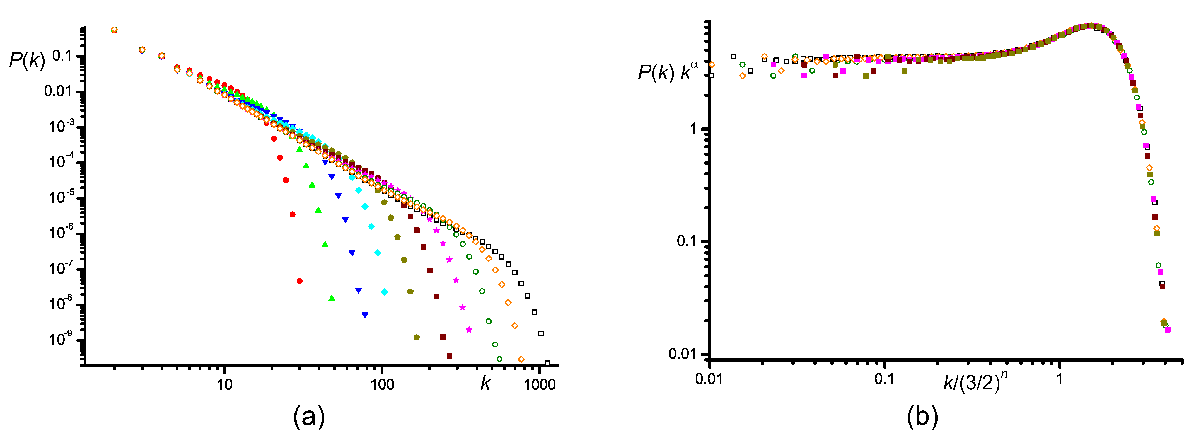
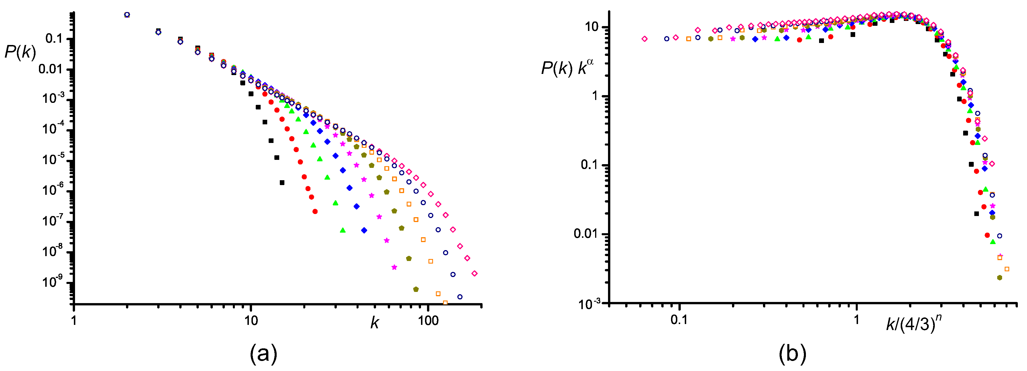
Once again, in order to check the predictions $2\times {10}^5$ realizations of the networks of up to the 12th generation were generated. The results are shown in Figure 5a, and in Figure 5b the plot in the renormalized coordinates is shown. The collapse of the data onto a single master curve is apparent, although it is somewhat worse than in Figure 3b. Presumably, this happens because the typical degrees in the hexagon-based network are much smaller than in the tetragon-network of the same size, and finite size effects are therefore more important.

4. Polygon-Based Networks with Smoothly Changing Exponent of the Degree Distribution

As a result of Section 3, one now has a sequence of Apollonian-like models that generate planar scale-free networks with a discrete sequence of degree-distribution exponents ${\alpha }_m=1+ln2/(ln(m+1)-lnm),m=2,3,\cdots$ Is it possible to further generalize the model to make $\alpha$ change continuously and take any intermediate values, including, for example, $\alpha =3$, corresponding to the point where the second moment of the degree distributions diverges for the first time?

It turns out that this is indeed possible. One way to do that is as follows. Assume that when introducing a new shortcut dividing a polygon in two, one makes the resulting partition to be a pair of tetragons with probability p and a pair of hexagons with probability $1-p$. That is to say, if the original polygon is a tetragon, then with probability p introduce a 2-step path connecting opposite vertices, and with probability $q=1-p$, a 4-step path; if the original polygon is a hexagon, the new path connecting two opposite vertices is a 1-step path with probability p and a 3-step path with probability q.

Here, we restrict ourselves to this simplest construction, although it is possible to create more complicated rules. For example, one can introduce correlations between generations in a Markovian way so that there is a matrix $p_{ij}$ of probabilities for a tetragon to give birth to a couple of tetragons, a hexagon to give birth to a couple of tetragons, etc. As a result, it might be possible to construct a network that is, for example, tetragon-dominated at large scales (early generations) and hexagon-dominated at small scales (later generations).

Once again, consider a node, which is created at generation $n_0$, and let us study its degree distribution at generation $n_0+n$. This degree distribution depends only on n and on the number of edges of the initial two faces adjacent to the node where tetragons or hexagons.

Let the average fraction of tetragons at a given generation be p and the fraction of hexagons be $q=1-p$. Then, for each face adjacent to a given node, the probability that this face is a tetragon is

$$\pi \left(p\right)=\frac{4p}{4p+6q}=\frac{2p}{3-p}.$$

(56)

Assume now that different faces adjacent to a node are tetragons (hexagons) independently from each other. Generally speaking, that is not true: when a new edge is created, the two faces on the sides of it have a similar number of edges. However, one might expect that as the degree of the node grows the correlations become less and less relevant. In this approximation, the probability for a node of degree k to have exactly l adjacent tetragons is

$$\left(\genfrac{}{}{0pt}{}{k}{l}\right){\pi }^l{(1-\pi )}^{k-l}.$$

(57)

when the next generation is created, a new edge adjacent to the node under consideration is created with probability $1/2$ for each tetragon face and with probability $1/3$ for each hexagon face. Therefore, one can write down the following approximate equation for the probability $P(k+r|k,p)$ of the node that has degree $k+r$ at the next generation given that it had degree k in the previous one:

$$P(k+r|k,p)=\sum _{l=0}^k\sum _{s=0}^r\left(\genfrac{}{}{0pt}{}{k}{l}\right){\pi }^l{(1-\pi )}^{k-l}\left(\genfrac{}{}{0pt}{}{l}{s}\right){\left(\frac{1}{2}\right)}^l\left(\genfrac{}{}{0pt}{}{k-l}{r-s}\right){\left(\frac{1}{3}\right)}^{r-s}{\left(\frac{2}{3}\right)}^{k-l-r+s},$$

(58)

where the binomial coefficients $\left(\genfrac{}{}{0pt}{}{m}{n}\right)$ are assumed to be zeros if $n>m$ or $n<0$. Now, introduce the probability $F_n\left(k\right|p)$ for a node to have degree k n generations after its creation, and the corresponding generation function,

$$f_n\left(\lambda \right|p)=\sum _{k=2}^{\infty }{F}_n\left(k\right){\lambda }^k.$$

(59)

Then, $f_0\left(\lambda \right|p)={\lambda }^2$,

$$F_n\left(k\right)=\sum _{k^{\prime }=\lfloor \frac{k+1}{2}\rfloor }^{k}P\left(k\right|k^{\prime },p)F_{n-1}\left(k^{\prime }\right),$$

(60)

and

$$f_n\left(\lambda \right|p)=\sum _{k=2}^{\infty }\sum _{k^{\prime }=\lfloor \frac{k+1}{2}\rfloor }^k{\lambda }^{k}P\left(k\right|k^{\prime },p)F_{n-1}\left(k^{\prime }\right)=\sum _{k^{\prime }=2}^{\infty }{F}_{n-1}\left(k^{\prime }\right){\lambda }^{k^{\prime }}\sum _{k=k^{\prime }}^{2k^{\prime }}{\lambda }^{k-k^{\prime }}P\left(k\right|k^{\prime },p).$$

(61)

Using Equation (58), it is easy to calculate the second sum on the right-hand side:

$$\begin{array}{ccc}\hfill {\sum }_{r=0}^{k^{\prime }}{\lambda }^{r}P(k^{\prime }+r|k^{\prime },p)& =\hfill & {\sum }_{r=0}^{k^{\prime }}{\sum }_{l=0}^{k^{\prime }}{\sum }_{s=0}^r\frac{k^{\prime }!}{s!(l-s)!(r-s)!(k^{\prime }-l-r+s)!}{\pi }^l{(1-\pi )}^{k^{\prime }-l}{\left(\frac{1}{2}\right)}^l{\left(\frac{1}{3}\right)}^{r-s}{\left(\frac{2}{3}\right)}^{k^{\prime }-l-r+s}{\lambda }^r\hfill \\ & =\hfill & {\sum }_{r=0}^{k^{\prime }}{\sum }_{l=0}^{k^{\prime }}{\sum }_{s=0}^r\frac{k^{\prime }!}{s!(r-s)!(l-s)!(k^{\prime }-l-r+s)!}{\left(\frac{\pi \lambda }{2}\right)}^s{\left(\frac{\pi }{2}\right)}^{l-s}{\left(\frac{(1-\pi )\lambda }{3}\right)}^{r-s}{\left(\frac{2(1-\pi )}{3}\right)}^{k^{\prime }-l-r+s}\hfill \\ & =\hfill & {\left(\frac{\pi \lambda }{2}+\frac{\pi }{2}+\frac{(1-\pi )\lambda }{3}+\frac{2(1-\pi )}{3}\right)}^{k^{\prime }},\hfill \end{array}$$

(62)

which leads to the following equation for the generating function:

$$f_n\left(\lambda \right)=f_{n-1}\left(\lambda \left(\frac{4-\pi }{6}+\frac{2+\pi }{6}\lambda \right)\right)=f_{n-1}\left(\frac{2-p+\lambda }{3-p}\lambda \right),$$

(63)

where Equation (56) is taken into account to obtain to the last expression. Proceeding as before, one gets the equation for the generating function of the full limiting degree distribution $g_{\infty }\left(\lambda \right)$ (except for the initial set of nodes):

$$g_{\infty }\left(\lambda \right)=\frac{{\lambda }^2}{2}+\frac{1}{2}{g}_{\infty }\left(\frac{2-p+\lambda }{3-p}\lambda \right).$$

(64)

Expanding $g_{\infty }\left(\lambda \right)$ for $\lambda =1-ϵ,ϵ\ll 1$ in the form (compare Equation (18)):

$$\overline{g}\left(\lambda \right)=\sum _{i=0}^{\lfloor \alpha \left(p\right)-1\rfloor }{a}_i{ϵ}^i+C\Gamma (1-\alpha \left(p\right)){ϵ}^{\alpha \left(p\right)-1}+o\left({ϵ}^{\alpha \left(p\right)-1}\right),$$

(65)

and equating the coefficients term by term exactly in the same way as in Section 2, one gets the following equation for the degree distribution exponent $\alpha \left(p\right)$:

$$2={\left(\frac{4-p}{3-p}\right)}^{\alpha \left(p\right)-1},\alpha \left(p\right)=1+\frac{ln2}{ln(4-p)-ln(3-p)}.$$

(66)

Thus, for example, the interesting case $\alpha \left(p\right)=3$ when the second moment of the degree distribution diverges for the first time corresponds to

$${p|}_{\alpha =3}=2-\sqrt{2}\approx 0.58579\cdots$$

(67)

In Figure 6, the numerical data for the degree distribution of the mixed networks are shown. One can clearly see that the slope of the distribution gradually changes with changing p. Moreover, after rescaling the degree distribution with the power law prescribed by Equation (66), all curves are approximately flat for small k, validating the approximation of independent phases.

5. Concluding Remarks and Open Questions

This paper presents one possible class of planar random graphs constructed from polygons with an even number of edges using a procedure similar to the construction of Apollonian graphs [18]. The $2m$-polygon-based graphs have a limiting power law degree distribution with the exponent,

$${\alpha }_m=1+\frac{ln2}{ln(m-1)-lnm},$$

(68)

and the moments of the degree distribution are given by Equations (21) and (55). The second moment of the degree distribution diverges as ${(9/8)}^n$ with the number of generations n in the case of tetragon-based graphs (see Equation (41)) and converges to a finite value in Equation (55) for the polygons with a larger number of edges. Moreover, as described in Section 4, it is possible to construct a mixed model based on two different polygons (tetragons and hexagons in our example) so that on all stages of construction, tetragons are formed with probability p and hexagons with probability $1-p$. By varying p, one can adjust the slope of the degree distribution in order to achieve a desired value in a way reminiscent of evolving Apollonian networks [26].

Clearly, all graph classes presented here are small world. Indeed, the diameter of the graphs grows at most linearly with the number of generations:

$$d_{n+1}\le d_n+2\lfloor m/2\rfloor ,$$

(69)

where $d_n$ is the diameter of the n-generation graph. In turn, the total number of nodes grows exponentially with the number of generations; thus, the diameter is, at most, proportional to the logarithm of the number of nodes.

The shortest cycles in the graphs presented here are $2m$, and, in particular, there are no triangles in them, so, generally speaking, the clustering coefficient is zero. However, this should not obscure the fact that there is actually a huge number of short cycles in these graphs. Indeed, consider the following auxiliary construction: let the polygon-based construction be exactly as presented above up to n-th generation, but then connect all the nodes belonging to the same face on the last generation of the procedure, so the smallest faces (i.e., faces constructed on the last step) are considered to be complete graphs $K_{2m}$ ($(2m-1)$-simplices). The large-scale structure of the resulting graph (including, e.g., the slope of the degree distribution) will be the same as in the original polygon-based procedure, but a finite fraction of nodes (those created in the n-th generation of the construction) will have clustering coefficient 1, guaranteeing that the average clustering coefficient of the whole graph remains finite as $n\to \infty$. In order to use polygon-based graphs as a toy model for experimental systems, it might be reasonable to add a random fraction of them in order to fit the observed clustering coefficient instead of adding all possible links connecting the vertices in the smallest faces.

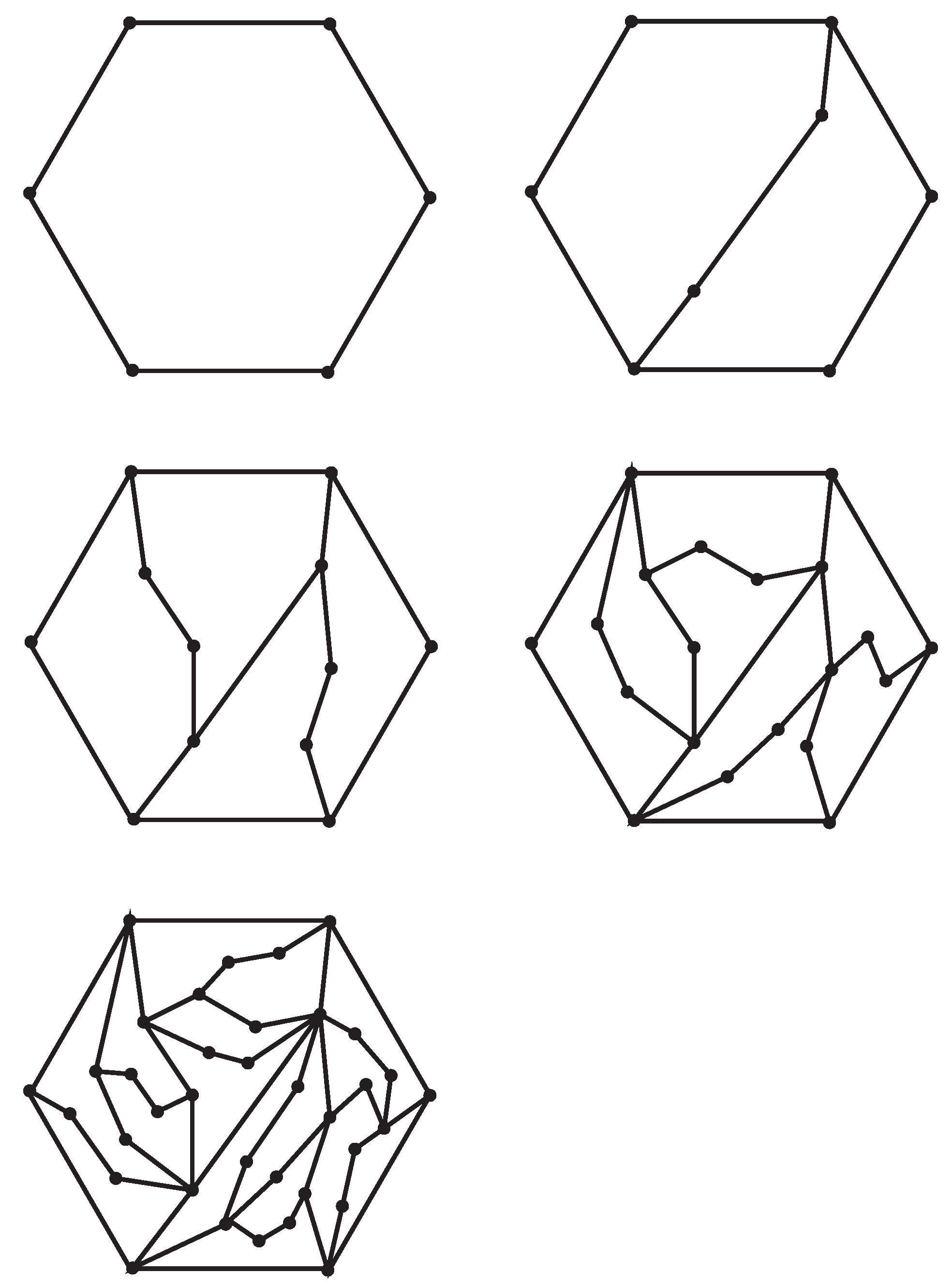
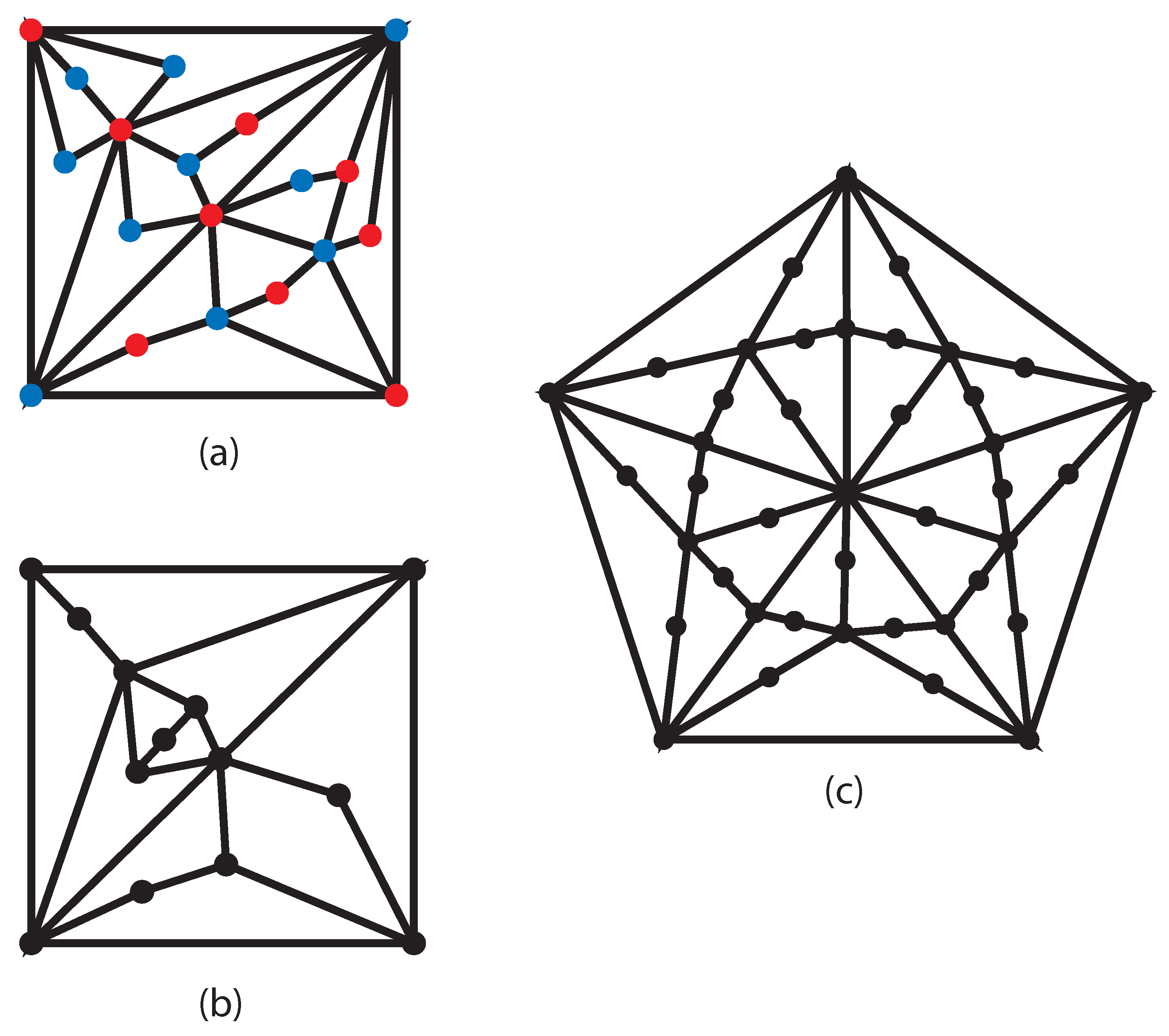
Interestingly, polygon-based graphs with even m are bipartite, see Figure 7a. In that sense, the tetragon-based graph seems to be a natural generalization of the Apollonian construction for the case of bipartite graphs. We expect that there might be a connection between bipartite polygon-based graphs and space-filling bearings, which allow only cycles of even lengths [37] in a way similar to the connection between original Apollonian networks and space-filling systems of embedded disks. Exploring this question goes, however, beyond the scope of this paper.

This paper restricts itself to just one class of possible generalizations of the Apollonian construction based on polygons of arbitrary sizes. It is quite easy to suggest various other generalizations. The most obvious example is, probably, the random polygon construction where new graphs are constructed not generation-by-generation by splitting all the polygons of the previous generation at once, but rather by randomly choosing on each step a face to split. Figure 7b presents an example realization of such a tetragon-based random graph. In the standard Apollonian case, it is known that the exponent of the degree distribution is different for the regular and random constructions. Calculating the degree distribution of random Apollonian-like polygon-based graphs remains an interesting open question.

Another, this time a completely deterministic generalization, is as follows. Consider a polygon with an odd number of edges $2m+1,m\ge 1$. Put a point inside the polygon and connect it with all vertices of the polygon by chains of m edges and $(m-1)$ nodes. This splits a polygon into $2m+1$ faces, each having exactly $2m+1$ edges. On the next step, repeat this procedure for each of the faces and proceed ad infinitum. Figure 7c shows the second-generation pentagon-based graph obtained via such procedure. Clearly, this construction is an even more direct generalization of the Apollonian graph construction (indeed, $m=1$ case is just the Apollonian graph itself). However, it means that it has standard drawbacks of the Apollonian graph in a sense that it is a single deterministic object rather than a stochastic ensemble of graphs and that its limiting degree distribution is not a power law but rather a log-periodic function with a power law envelope.

We think that the classes of graphs presented here are a useful addition to the toolkit of toy models to model scale-free graphs. Indeed, while having the main advantages of the Apollonian networks, they have additional flexibility in a sense that one might regulate the slope of the degree distribution and the average clustering coefficient in the way described above. In particular, such graphs might be, in our opinion, useful in the applications where graph planarity is essential [38], for example, in quantitative geography, such as the study of the formation of the systems of interconnected cities. On the other side, studying percolation, spectral properties, diffusion, synchronization, epidemic spreading, etc., on these generalized graphs might allow to systematically study the influence of varying degree exponents on these phenomena, which, to the best of our knowledge, have not yet been done for the scale-free planar networks.

References

1. Tikhonov, K.S.; Mirlin, A.D. From Anderson localization on random regular graphs to many-body localization. Ann. Phys. 2021, in press. [Google Scholar] [CrossRef]
2. Sneppen, K.; Zocchi, G. Physics in Molecular Biology; Cambridge University Press: Cambridge, UK, 2005. [Google Scholar] [CrossRef]
3. Jackson, M.O. Social and Economic Networks; Princeton University Press: Princeton, NJ, USA, 2010. [Google Scholar]
4. Kenett, Y.N.; Anaki, D.; Faust, M. Investigating the structure of semantic networks in low and high creative persons. Front. Hum. Neurosci. 2014, 8, 407. [Google Scholar] [CrossRef] [PubMed] [Green Version]
5. Stella, M.; Beckage, N.M.; Brede, M.; Domenico, M.D. Multiplex model of mental lexicon reveals explosive learning in humans. Sci. Rep. 2018, 8, 2259. [Google Scholar] [CrossRef] [PubMed] [Green Version]
6. Valba, O.V.; Gorsky, A.S.; Nechaev, S.K.; Tamm, M.V. Analysis of English free association network reveals mechanisms of efficient solution of Remote Association Tests. PLoS ONE 2021, 16, e0248986. [Google Scholar]
7. Newman, M. Networks; Oxford University Press: Oxford, UK, 2018. [Google Scholar] [CrossRef]
8. Barabasi, A.L. Network Science; Cambridge University Press: Cambridge, UK, 2016. [Google Scholar]
9. Dorogovtsev, S. Complex Networks; Oxford University Press: Oxford, UK, 2010. [Google Scholar] [CrossRef]
10. Erdős, P.; Rényi, A. On Random Graphs I. Publ. Math. 1959, 6, 290–297. [Google Scholar]
11. Krapivsky, P.L.; Redner, S.; Ben-Naim, E. A Kinetic View of Statisrical Physics; Cambridge University Press: Cambridge, UK, 2010. [Google Scholar] [CrossRef] [Green Version]
12. Balister, P.; Bollobás, B.; Sarkar, A. Percolation, connectivity, coverage and colouring of random geometric graphs. In Handbook of Large-Scale Random Networks; János Bolyai Mathematics Society Studies; Bollobás, B., Kozma, R., Miklós, D., Eds.; Springer: Berlin/Heidelberg, Germany, 2008. [Google Scholar] [CrossRef]
13. Barabási, A.L.; Albert, R. Emergence of scaling in random networks. Science 1999, 286, 509–512. [Google Scholar] [CrossRef] [Green Version]
14. Watts, D.; Strogatz, S. Collective dynamics of ‘small-world’ networks. Nature 1998, 393, 440–442. [Google Scholar] [CrossRef]
15. Krioukov, D.; Papadopoulos, F.; Kitsak, M.; Vahdat, A.; Boguna, M. Hyperbolic geometry of complex networks. Phys. Rev. E 2010, 82, 036106. [Google Scholar] [CrossRef] [Green Version]
16. Boguna, M.; Papadopoulos, F.; Krioukov, D. Sustaining the internet with hyperbolic mapping. Nat. Commun. 2010, 1, 62. [Google Scholar] [CrossRef] [Green Version]
17. Papadopoulos, F.; Kitsak, M.; Serrano, M.Á.; Boguná, M.; Krioukov, D. Popularity versus similarity in growing networks. Nature 2012, 489, 537–540. [Google Scholar] [CrossRef] [Green Version]
18. Andrade, J.S., Jr.; Herrmann, H.J.; Andrade, R.F.S.; da Silva, L. Apollonian networks: Simultaneously scale-free, small world, Euclidean, space filling, and with matching graphs. Phys. Rev. Lett. 2005, 94, 018702. [Google Scholar] [CrossRef] [Green Version]
19. Doye, J.P.K.; Massen, C.P. Self-similar disk packings as model spatial scale-free networks. Phys. Rev. E 2005, 71, 016128. [Google Scholar] [CrossRef] [PubMed] [Green Version]
20. Kasner, E.; Supnick, F. The Apollonian packing of circles. Proc. Natl. Acad. Sci. USA 1943, 29, 378–384. [Google Scholar] [CrossRef] [PubMed] [Green Version]
21. Boyd, D.W. The residual set dimension of the Apollonian packing. Mathematika 1973, 20, 170–174. [Google Scholar] [CrossRef]
22. Zhang, Z.; Chen, L.; Zhou, S.; Fang, L.; Guan, J.; Zou, T. Analytical solution of average path length for Apollonian networks. Phys. Rev. E 2008, 77, 017102. [Google Scholar] [CrossRef] [PubMed] [Green Version]
23. Bianconi, G.; Ziff, R.M. Topological percolation on hyperbolic simplicial complexes. Phys. Rev. E 2018, 98, 052308. [Google Scholar] [CrossRef] [Green Version]
24. Andrade, R.F.S.; Hermann, H.J. Magnetic models on Apollonian networks. Phys. Rev. E 2005, 71, 056131. [Google Scholar] [CrossRef] [Green Version]
25. Lind, P.G.; da Silva, L.R.; Andrade, J.S., Jr.; Hermann, H.J. Spreading gossip in social networks. Phys. Rev. E 2007, 76, 036117. [Google Scholar] [CrossRef] [Green Version]
26. Zhang, Z.; Rong, L.; Zhou, S. Evolving Apollonian networks with small-world scale-free topologies. Phys. Rev. E 2006, 74, 046105. [Google Scholar] [CrossRef] [Green Version]
27. Mendes, G.A.; da Silva, L.R.; Hermann, H.J. Traffic gridlock on complex networks. Phys. A 2012, 391, 362. [Google Scholar] [CrossRef] [Green Version]
28. Huang, Z.-G.; Xu, X.-J.; Wu, Z.-X.; Wang, Y.-H. Walks on Apollonian networks. Eur. Phys. J. B 2006, 51, 549–553. [Google Scholar] [CrossRef] [Green Version]
29. Zhang, Z.; Guan, J.; Xie, W.; Qi, Y.; Zhou, S. Random walks on the Apollonian network with a single trap. Europhys. Lett. 2009, 86, 10006. [Google Scholar] [CrossRef]
30. Newberry, M.G.; Savage, V.M. Self-similar processes follow a power law in discrete logarithmic space. Phys. Rev. Lett. 2019, 122, 158303. [Google Scholar] [CrossRef] [PubMed] [Green Version]
31. Zhou, T.; Yan, G.; Zhou, P.-L.; Fu, Z.-Q.; Wang, B.-H. Random apollonian networks. arXiv 2004, arXiv:0409414. [Google Scholar]
32. Zhou, T.; Yan, G.; Wang, B.-H. Maximal planar networks with large clustering coefficient and power-law degree distribution. Phys. Rev. E 2005, 71, 046141. [Google Scholar] [CrossRef] [PubMed] [Green Version]
33. Kolossvary, I.; Komjathy, J.; Vago, L. Degrees and distances in random and evolving Apollonian networks. Adv. Appl. Prob. 2016, 48, 865–902. [Google Scholar] [CrossRef] [Green Version]
34. Zhang, Z.; Comellas, F.; Fertin, G.; Rong, L. High-dimensional Apollonian networks. J. Phys. A 2006, 39, 1811. [Google Scholar] [CrossRef] [Green Version]
35. Zhang, Z.; Rong, L.; Comellas, F. High-dimensional random Apollonian networks. Phys. A 2006, 364, 610–618. [Google Scholar] [CrossRef] [Green Version]
36. Setna, J.P. Statistical Mechanics: Entropy, Order Parameters, and Complexity; Oxford University Press: Cambridge, UK, 2006. [Google Scholar] [CrossRef]
37. Oron, G.; Herrmann, H.J. Generalization of space-filling bearings to arbitrary loop size. J. Phys. A 2000, 33, 1417–1434. [Google Scholar] [CrossRef] [Green Version]
38. Barthelemy, M. Spatial networks. Phys. Rep. 2011, 499, 1–101. [Google Scholar] [CrossRef] [Green Version]
Figure 1. Apollonian network: (a) first (black) and second (black and red) generations of the Apollonian network; (b) first generation of the same Apollonian network represented as a tetrahedron in 3-dimensional space; (c) Apollonian networks of higher generations can be thought of as rooted trees constructed from adjacent tetrahedra. Here, second generation is shown; the shaded face functions as a root of the tree.
Physics 03 00063 g001
Figure 2. Constructionof a tetragon-based network: (A) representatives of the tetragon-networks up to the 4th generation; (B) three possible topologically different realizations of the second-generation network; (C) random triangulation of the fourth-generation network.
Physics 03 00063 g002
Figure 3. (a) Degree distributions of the tetragon-based networks of generations 5–14 as indicated. The results shown are obtained after averaging over 2 × 10 5 realizations and logarithmic binning with step 1.1. (b) Same distributions but rescaled as the axes show.
Physics 03 00063 g003
Figure 4. Construction of the hexagon-based network (up to 4th generation).
Physics 03 00063 g004
Figure 5. (a) Degree distributions of the hexagon-based networks of generations 4–12 as indicated. The results shown are obtained after averaging over 2 × 10 5 realizations and logarithmic binning with step 1.1. (b) Same distributions but rescaled as the axes show.
Physics 03 00063 g005
Figure 6. (a) Degree distributions of n = 10 th-generation mixed tetragon–hexagon networks with varying p, rainbow changing color from p = 0.9 (red) to p = 0.1 (violet). The results shown are obtained after averaging over 10 5 realizations and logarithmic binning with step 1.05. (b) Same distributions but rescaled: P ( k ) is rescaled by its theoretical behavior k α , with α given by Equation (66), k is rescaled by a factor k 0 ( p , n ) = ( ( 4 p ) / ( 3 p ) ) n , which approximates the growth of the maximal accessible degree with the number of generations n.
Physics 03 00063 g006
Figure 7. (a) Tetragon-based networks are bipartite. (b) An example of a particular realization of a randon tetragon-based graph. (c) An example of a 2nd-generation deterministic pentagon-based graph.
Physics 03 00063 g007
Publisher’s Note: MDPI stays neutral with regard to jurisdictional claims in published maps and institutional affiliations.