Article

Multi-Sensor Fusion-Based Autonomous Navigation for a Tracked Agricultural Chassis in Hilly Farmland: Python and ROS/Gazebo Simulation Validation

Mechanical and Electrical Engineering, Yunnan Agricultural University, Kunming 650201, China
*
Author to whom correspondence should be addressed.
AgriEngineering 2026, 8(6), 231; https://doi.org/10.3390/agriengineering8060231
Submission received: 3 May 2026 / Revised: 30 May 2026 / Accepted: 2 June 2026 / Published: 5 June 2026

Abstract

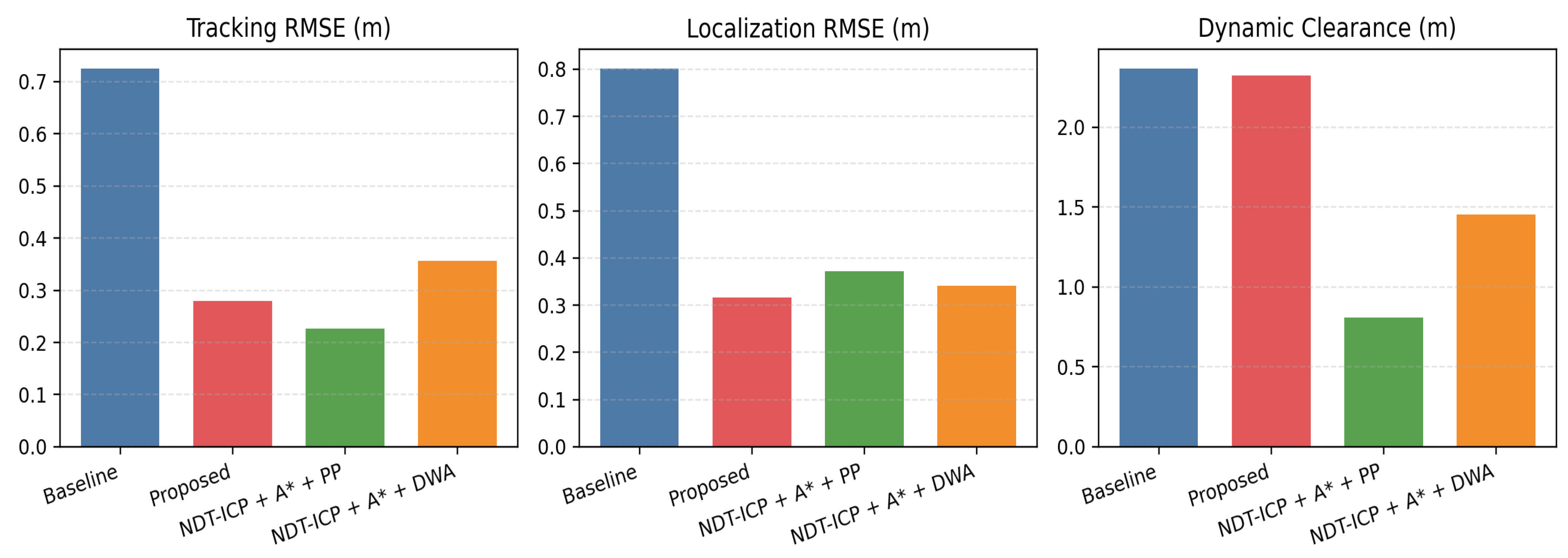
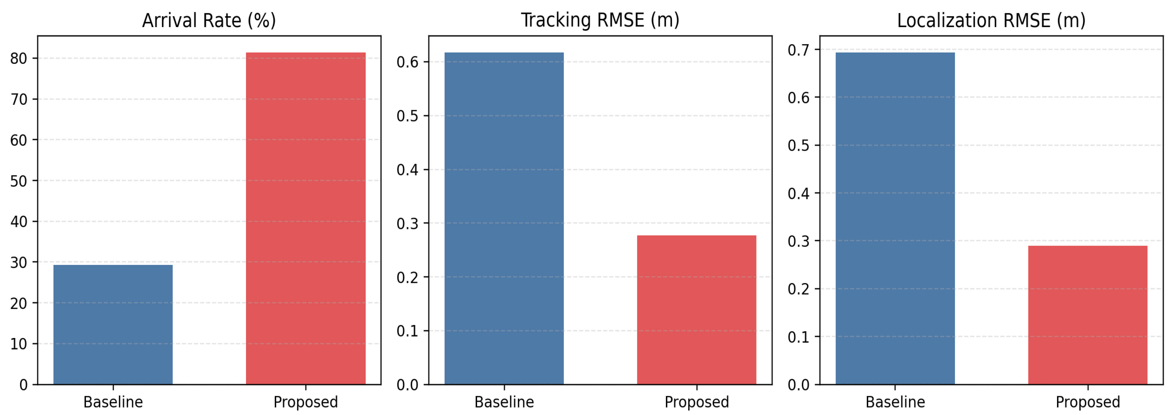
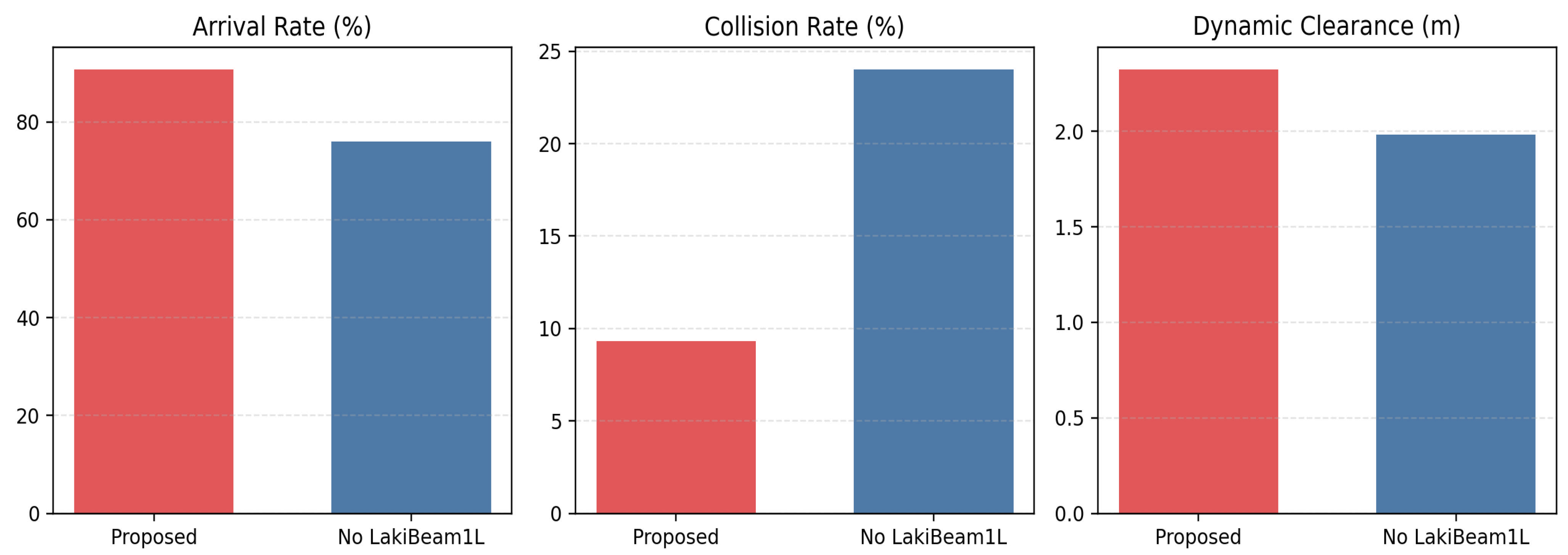
This paper proposes a multi-sensor fusion autonomous navigation method integrating a nine-axis IMU, the Leishen C16 mechanical LiDAR, and the LakiBeam1L single-line LiDAR, aimed at addressing issues such as track slippage and positioning drift that commonly occur in tracked chassis operating under continuously changing conditions on hilly slopes and farmland. IMU-derived slope and attitude information is used as a terrain prior and incorporated into adaptive ground segmentation, slope-cross-slope path cost modeling, and velocity regulation. Leishen C16 LiDAR point clouds are used for NDT scan-to-map localization and spatial obstacle representation, while the LakiBeam1L LiDAR establishes a velocity-dependent near-field safety zone for dynamic obstacle triggering and local avoidance. Python simulations were conducted in simple, general, and complex environments under five slope conditions, forming 15 environment-slope combinations. Three representative scenarios were further validated in ROS/Gazebo. To strengthen statistical reliability, 10 repeated trials were performed for each environment-slope-algorithm combination, and additional stress tests included obstacle-position perturbation, sensor noise perturbation, initial-pose perturbation, dynamic obstacle speed perturbation, and variable slope/local undulation perturbation. An isolated no-LakiBeam1L ablation, significance tests, IMU perturbation tests, planning-weight sensitivity analysis, and stronger-baseline comparison were also added. In the repeated-trial dataset, the proposed method improved the arrival rate from 23.3% to 94.7%, reduced tracking RMSE by 61.46%, reduced localization RMSE by 60.62%, and increased obstacle recall by 26.32%. Under mixed perturbations, the arrival rate of the proposed method was 81.3%, compared with 29.3% for the baseline. These results indicate improved simulation-level stability and perception reliability, while the applicability to real hilly farmland still requires hardware and field validation.

1. Introduction

Application scenarios such as agricultural operations on hilly slopes, forest land inspections, and mountain transportation impose higher demands on the autonomous navigation capabilities of mobile robots. Compared with regular roads or flat farmland, hilly farmland is characterized by continuously varying slopes, significant cross-slope risks, uneven ground surfaces, irregular obstacle distributions, and frequent occlusion of perception information. These factors lead to stronger coupling among environmental perception, pose estimation, path planning, and motion control. For tracked chassis, changes in slope adhesion, track slip, and steering stability directly affect terrain passability and navigation reliability [1]. In addition, autonomous navigation systems for agricultural machinery generally involve environmental perception, path planning, and path-tracking control, while their engineering application is still constrained by unstructured terrain, complex obstacles, and mechanical motion stability [2]. In recent years, agricultural robot navigation has gradually evolved from single-sensor-driven and single-module optimization toward multi-sensor fusion, complex-environment perception, and coordinated planning–control design. However, in open fields, constrained working areas, and unstructured agricultural environments, localization stability, obstacle-detection robustness, and safe path tracking remain key bottlenecks for practical deployment [3,4,5].
In environmental perception and mapping, LiDAR SLAM, visual navigation, and laser-inertial fusion positioning have become key technical approaches for navigating agricultural robots in complex environments. Jiang et al., Hong et al., and Huang et al. improved localization stability from the perspectives of 3D LiDAR SLAM with NDT-ICP point cloud registration, LiDAR–inertial odometry, and improved FAST-LIO2-based greenhouse navigation, respectively [6,7,8]. In addition, stereo vision, 2D LiDAR SLAM, spatial LiDAR odometry and mapping, adaptive LiDAR odometry, and LiDAR/IMU/GNSS integrated navigation have also been applied to orchard, greenhouse, and unmanned farm scenarios [9,10,11,12,13]. These studies indicate that multi-source perception and point cloud constraints can effectively improve localization and mapping performance in complex agricultural environments. However, most existing studies still focus on orchards, greenhouses, unmanned farms, and relatively regular agricultural scenarios. Insufficient attention has been paid to localization drift caused by the combined effects of continuously varying slopes, surface undulation, and cross-slope risks in hilly farmland.
In path planning and risk modeling, agricultural robot navigation has gradually shifted from a shortest-path-oriented strategy to integrated optimization that considers traversability, safety, and stability. Previous studies have combined improved A* and fuzzy DWA algorithms for mobile robot path planning in greenhouse orchards [14]. Other studies have explored risk-aware traversability learning [15], traversability analysis combined with RRT* [16], improved D* Lite hybrid planning [17], LiDAR-based obstacle identification and mapping, and octree-based 3D point cloud optimization [18,19] to improve path feasibility and obstacle avoidance in complex agricultural environments. These studies provide an important basis for path generation and risk avoidance in agricultural scenarios. Nevertheless, under hilly farmland conditions with continuous slope variation and significant cross-slope risks, existing planning models remain insufficient in the unified modeling of terrain traversability, cross-slope risk, and obstacle-related safety cost.
In terms of path tracking and vehicle control, tracked or skid-steering agricultural platforms exhibit longitudinal slip, lateral sideslip, and nonlinear steering characteristics. Conventional fixed-parameter tracking methods may suffer from amplified tracking errors and reduced stability during curved-path tracking, headland turning, and operation on complex ground surfaces. Existing studies have investigated improved Pure Pursuit for brake-steering tracked vehicles, model-free adaptive predictive control, adaptive look-ahead distance adjustment for crawler tractors, path tracking for paddy-field weeders, adaptive control for unmanned crawler harvesters, slip-aware look-ahead point offset, and adaptive backstepping control under longitudinal slip conditions [20,21,22,23,24,25,26]. These studies demonstrate that adjusting tracking parameters according to vehicle states and ground adhesion conditions is important for improving the control stability of tracked platforms. However, in hilly farmland, the controller must consider not only path curvature and lateral error but also slope variation, attitude disturbance, and near-field dynamic obstacle safety triggering within a unified control logic. Otherwise, under the combined effects of steep slopes, sharp turns, and dynamic obstacles, a tracked chassis may still suffer from excessive speed, steering oscillation, increased sideslip, or insufficient safety clearance.
Overall, existing agricultural robot navigation methods have achieved promising performance in structured and semi-structured agricultural environments. However, several limitations remain. First, most studies focus on orchard rows, greenhouses, high-bed cultivation, or general unstructured farmland, while scenarios with continuously varying slopes, significant cross-slope risks, and strongly undulating terrain have not been sufficiently addressed. Second, existing studies often optimize a single module, such as localization and mapping, obstacle detection, path planning, or path tracking, whereas systematic research on full-chain coordination among perception, localization, planning, and control for tracked chassis in sloped environments remains limited. Third, for common problems in hilly terrain, including track slip, localization drift, slope-induced point cloud misclassification, and near-field safety triggering for dynamic obstacles, a unified closed-loop solution is still lacking. The key challenge of autonomous navigation for tracked chassis in hilly farmland is not merely the insufficient performance of a single module, but the coupled effects of slope variation, track slip, ground point cloud misclassification, and dynamic obstacle disturbance. To address these issues, this study focuses on a tracked agricultural chassis operating in hilly farmland and proposes a multi-sensor fusion autonomous navigation method integrating a nine-axis IMU, a Leishen C16 mechanical LiDAR, and a LakiBeam1L single-line LiDAR.
The proposed method introduces slope attitude priors, point cloud geometric constraints, slope–cross-slope path cost modeling, and velocity-dependent near-field safety control into a unified closed-loop navigation framework. The main contributions of this study are as follows:
  • To address localization drift caused by track slip and accumulated odometry errors in hilly farmland, an IMU slope attitude prior-aided NDT scan-to-map localization method is constructed. IMU attitude information is used to constrain the initial point cloud matching pose, while Leishen C16 LiDAR point cloud geometry is used to correct pose estimation, thereby improving localization stability on sloped terrain.
  • To address the problem that fixed-threshold ground segmentation may incorrectly classify continuous sloped ground as obstacles, an adaptive Ray Ground Filter method based on IMU-derived slope information is proposed. This method converts slope attitude information into an adaptive ground continuity threshold, thereby reducing false obstacle detection caused by continuous sloped ground.
  • To address the limitation that conventional distance cost planning cannot represent slope and cross-slope risks, a slope–cross-slope joint path cost model is developed. The model integrates path length, slope risk, cross-slope risk, and obstacle-distance cost to guide the planner toward safer and more executable paths in hilly farmland.
  • To reduce sideslip, trajectory oscillation, and insufficient dynamic safety clearance caused by fixed-speed tracking on sloped terrain, a path-tracking and safety control method integrating slope-based velocity regulation, heading error constraints, and a LakiBeam1L-based near-field safety zone is proposed. This strategy enables the chassis to reduce speed or trigger local avoidance when slope risk, steering demand, or dynamic obstacle risk increases.

2. Materials and Methods

2.1. System Overview

2.1.1. Platform Configuration

Hilly farmland is typically characterized by continuously varying slopes, uneven ground surfaces, variable soil adhesion, and irregular obstacle distributions. These environmental conditions impose high requirements on the terrain adaptability, traction stability, and motion robustness of agricultural mobile platforms. Compared with wheeled platforms, tracked chassis provide a larger ground-contact area and stronger terrain adaptability, making them more suitable for sloped and uneven farmland. Therefore, a tracked agricultural chassis was selected as the mobile platform in this study.
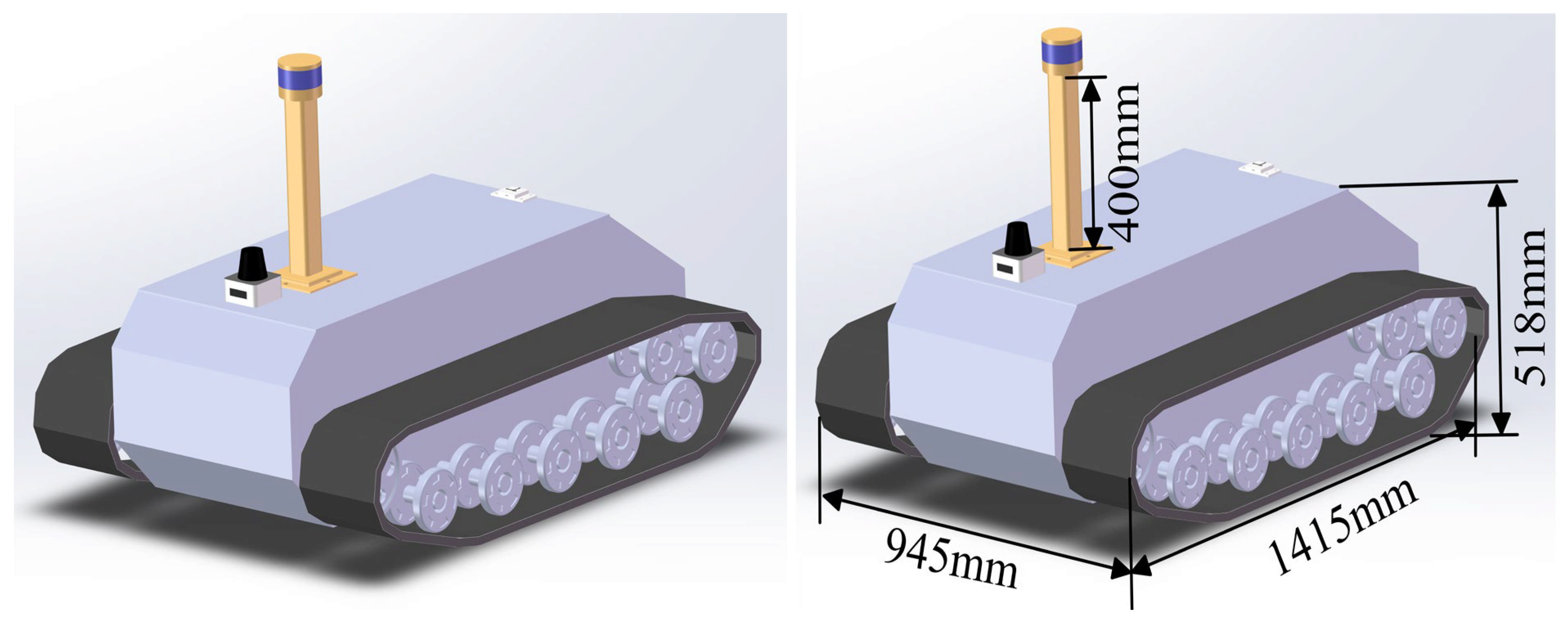
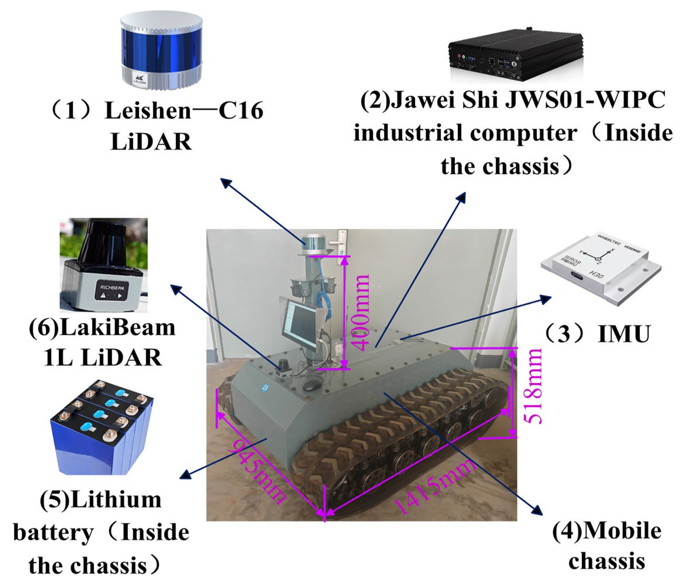
The integrated tracked chassis platform is shown in Figure 1. The platform consists of a mobile chassis, a Leishen C16 mechanical LiDAR, a nine-axis IMU, a LakiBeam1L single-line LiDAR, a lithium battery, and an industrial computer.
The industrial computer was a JWS01-WIPC unit supplied by Jiaweishi Electronic Technology Co., Ltd. (Shenzhen, China). The nine-axis IMU inertial navigation module was supplied by Wheeltec Technology Co., Ltd. (Dongguan, China). The Leishen C16 mechanical LiDAR was supplied by Leishen Technology (Shenzhen) Co., Ltd. (Shenzhen, China), and the LakiBeam1L single-line LiDAR was supplied by Richbeam Laser Technology Co., Ltd. (Beijing, China). The tracked chassis and lithium battery were selected according to the platform configuration, load capacity, installation space, and simulation requirements. The Leishen C16 mechanical LiDAR was mounted above the chassis at a height of 0.40 m to acquire three-dimensional point clouds and two-dimensional scan data. The IMU was fixed on the upper part of the chassis at a height of 0.51 m to provide roll, pitch, and heading information. The LakiBeam1L single-line LiDAR was mounted at the front of the chassis at a height of 0.518 m for near-field dynamic obstacle detection. The lithium battery was installed inside the chassis body, and the industrial computer was mounted inside the chassis to receive sensor data, execute navigation algorithms, and output motion-control commands.
The main parameters of the tracked chassis are listed in Table 1. The chassis adopts a four-channel composite damping suspension, which reduces vibration induced by uneven terrain and improves the stability of LiDAR-based mapping and point cloud processing. The chassis has an overall size of 1415 mm × 945 mm × 518 mm, a track width of 150 mm, a maximum obstacle-crossing height of 200 mm, a maximum trench-crossing capability of 400 mm, an operating speed range of 0–5.4 km/h, a rated load capacity of 300 kg, and a maximum climbing capability of no more than 30°.
The sensor configuration and functions are summarized in Table 2. The Leishen C16 mechanical LiDAR provides point cloud information for mapping, localization, ground segmentation, and obstacle representation. The IMU provides attitude and slope priors for point cloud compensation, slope-adaptive segmentation, path cost modeling, and velocity regulation. The LakiBeam1L single-line LiDAR is used for forward near-field dynamic obstacle detection and safety triggering.

2.1.2. Overall Navigation Architecture

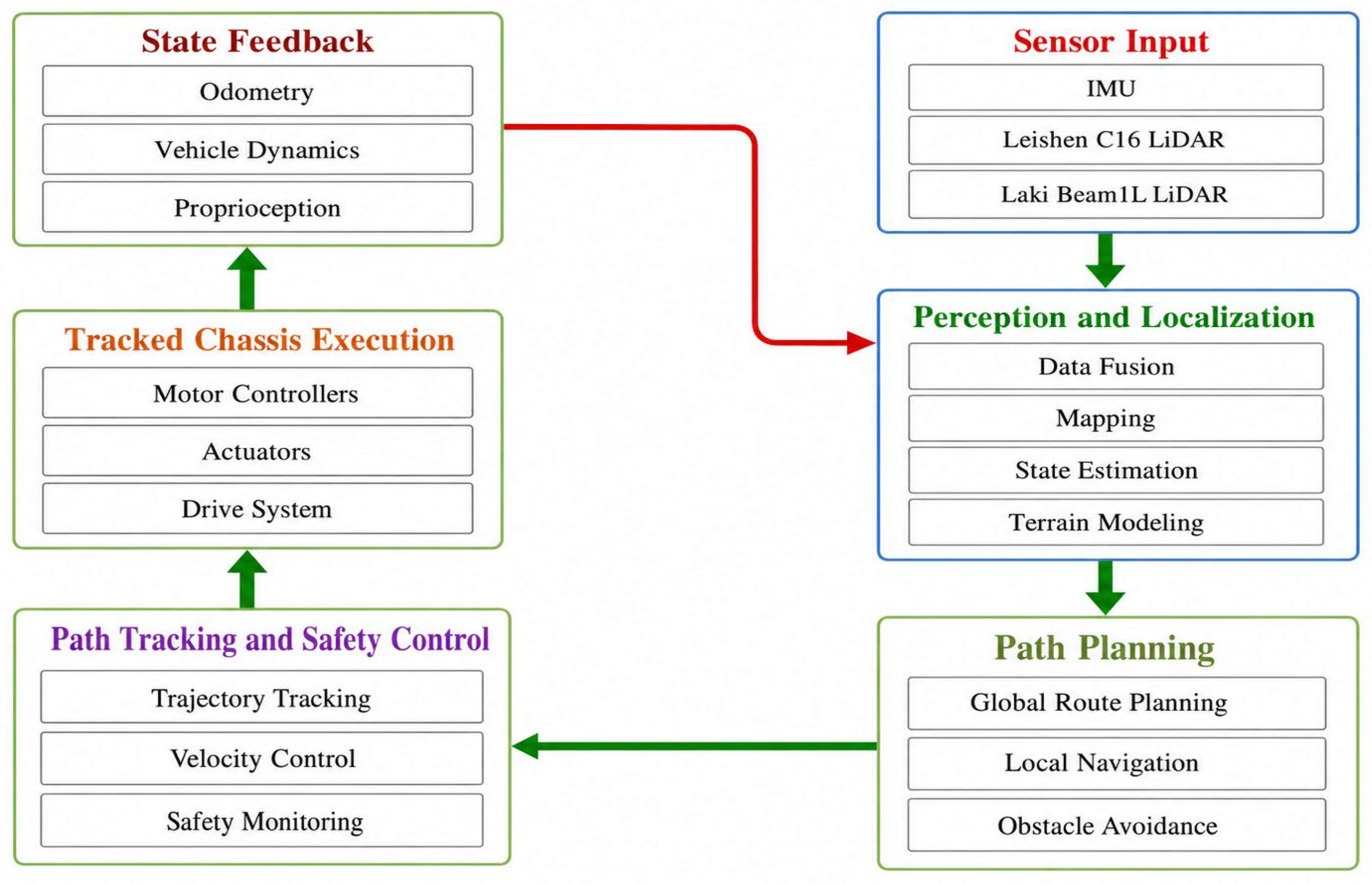
To achieve stable autonomous navigation in hilly farmland, the proposed system integrates an IMU, a Leishen C16 mechanical LiDAR, and a LakiBeam1L single-line LiDAR. The IMU provides slope and attitude information, the Leishen C16 LiDAR provides three-dimensional point clouds and two-dimensional scan data, and the LakiBeam1L LiDAR provides near-field dynamic obstacle safety triggering. Based on these sensing units, this study constructs a closed-loop navigation architecture consisting of slope attitude priors, point cloud geometric constraints, safety cost planning, and velocity-adaptive control.
The overall navigation workflow is shown in Figure 2. First, the IMU outputs attitude angles and estimates the equivalent slope angle, while the Leishen C16 LiDAR acquires environmental point clouds and the LakiBeam1L LiDAR monitors the forward near-field region. The point cloud data are transformed into a unified coordinate system and processed for ground segmentation and obstacle clustering. In the localization layer, IMU-aided NDT scan-to-map matching is used to correct the predicted pose. In the planning layer, a slope–cross-slope joint path cost model is introduced for global path planning, and local re-planning is triggered when a dynamic obstacle enters the near-field safety zone. In the control layer, Pure Pursuit tracking is combined with slope-adaptive velocity regulation and safety-triggered speed constraints. The chassis then executes the motion commands, and its state is fed back to the perception, planning, and control modules, forming a closed-loop autonomous navigation process.

2.2. Simulation Platform and Scenario Modeling

2.2.1. SolidWorks Modeling and Simplification

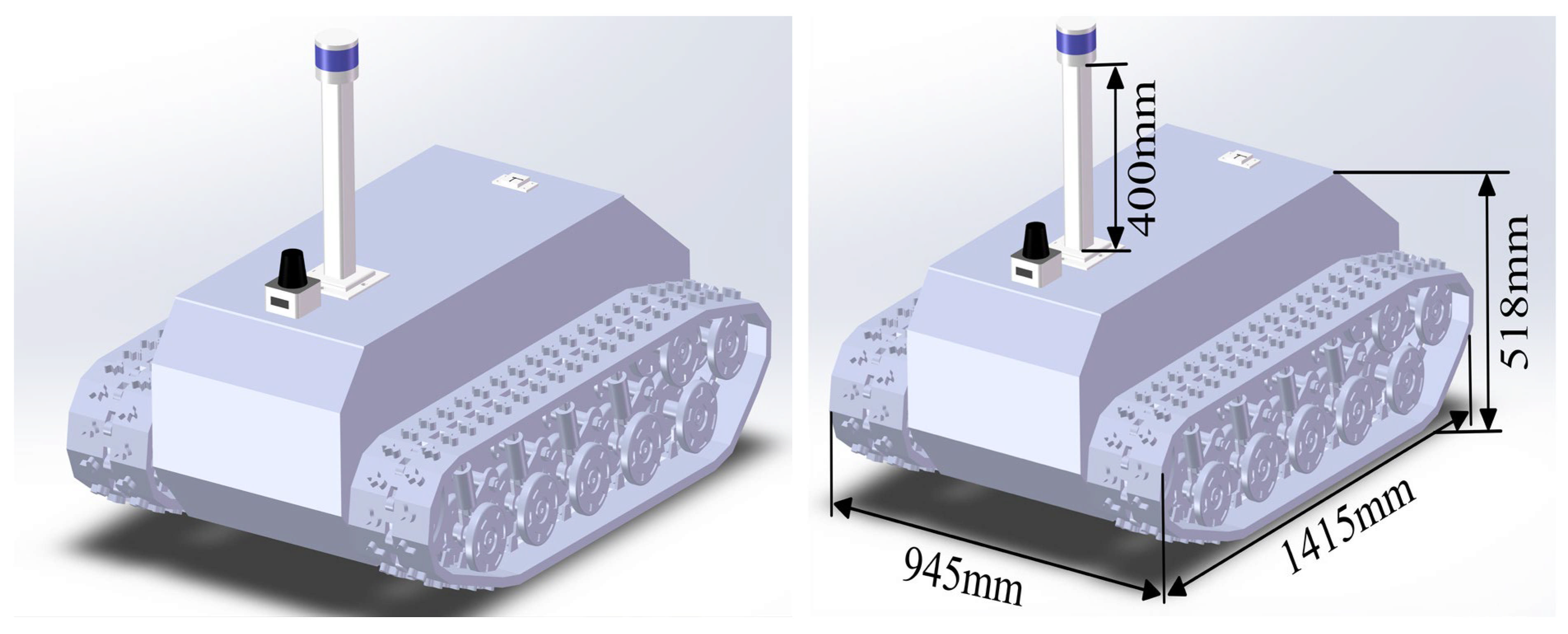
To construct the simulation platform for ROS/Gazebo, a three-dimensional model of the tracked chassis was first established in SolidWorks. The model included the chassis body, left and right tracks, drive motors, damping components, shafts, support wheels, driving wheels, carrier rollers, guide wheels, and sensor mounting components. The installation positions of the Leishen C16 mechanical LiDAR, the LakiBeam1L single-line LiDAR, and the IMU were determined according to the physical platform configuration. The complete assembly model is shown in Figure 3.
The SolidWorks model was exported as a URDF model using the sw2urdfSetup plug-in. This process improves modeling efficiency and reduces manual modeling errors. However, directly importing the complete URDF model into Gazebo may lead to abnormal collision solving, structural vibration, unstable simulation, and high computational cost because the Gazebo physics engine has limited capability in handling complex flexible track structures and small mechanical components. Therefore, the model was simplified before export. The simplification retained key components related to chassis kinematics, external dimensions, approximate mass distribution, and sensor installation, while removing or weakening small structures that had limited influence on navigation simulation. The simplified model was used to improve collision-calculation efficiency and simulation stability, as shown in Figure 4.

2.2.2. Hilly Farmland Simulation Scenario Modeling

This study used both Python simulation and ROS/Gazebo simulation for validation. The two simulation platforms serve different purposes. Python simulation was used to conduct statistical comparisons under controlled geometric conditions with multiple environments and slope settings. ROS/Gazebo simulation was used to verify the operational consistency of the tracked chassis model, sensor installation, trajectory visualization, and navigation workflow in an engineering simulation environment.
The Python simulation area was set to 30 m × 20 m. Three types of environments were constructed: simple, general, and complex. The simple environment contained three static circular obstacles and one dynamic obstacle; the general environment contained nine static circular obstacles and one dynamic obstacle; and the complex environment contained fifteen static circular obstacles and one dynamic obstacle. For each environment, five constant slopes of 5°, 10°, 15°, 20°, and 25° were considered. In each environment–slope combination, the slope angle remained constant, allowing the influence of slope variation on algorithm performance to be evaluated under controlled conditions.
The ROS/Gazebo simulation model was built using the simplified URDF model exported from SolidWorks. The Gazebo terrain consisted of a flat transition section and a constant-slope section. The slope values of 5°, 10°, 15°, 20°, and 25° reported in this paper refer to the nominal slope angle of the main constant-slope section rather than the average slope of the entire scene. A short transition section was placed between the flat ground and the slope to prevent physically unrealistic impact or contact discontinuity when the chassis entered the slope. To avoid confusion with the constant-slope Python simulation, the ROS/Gazebo results were used only for engineering visualization validation of representative scenarios and were not intended to replace the full statistical results obtained from Python simulation.

2.2.3. Software and Tool Versions

The Python batch simulations and post-processing scripts were executed under Python 3.12.0 on Windows 11. The main Python packages included NumPy 2.4.3, pandas 3.0.1, Matplotlib 3.10.8, SciPy 1.17.1, scikit-learn 1.8.0, and python-docx 1.2.0. The ROS/Gazebo representative simulations were implemented in Ubuntu 20.04 with ROS Noetic Ninjemys, ROS version 1.16.0, Gazebo 11, and RViz 1.14. The tracked chassis model was created in SolidWorks 2024 SP0.1 and exported with the SolidWorks-to-URDF Exporter (SW2URDF) version 1.6.0, build 1.6.7995.38578. The local A* verification script was prepared for MATLAB R2024b.

2.3. Multi-Sensor Fusion Framework

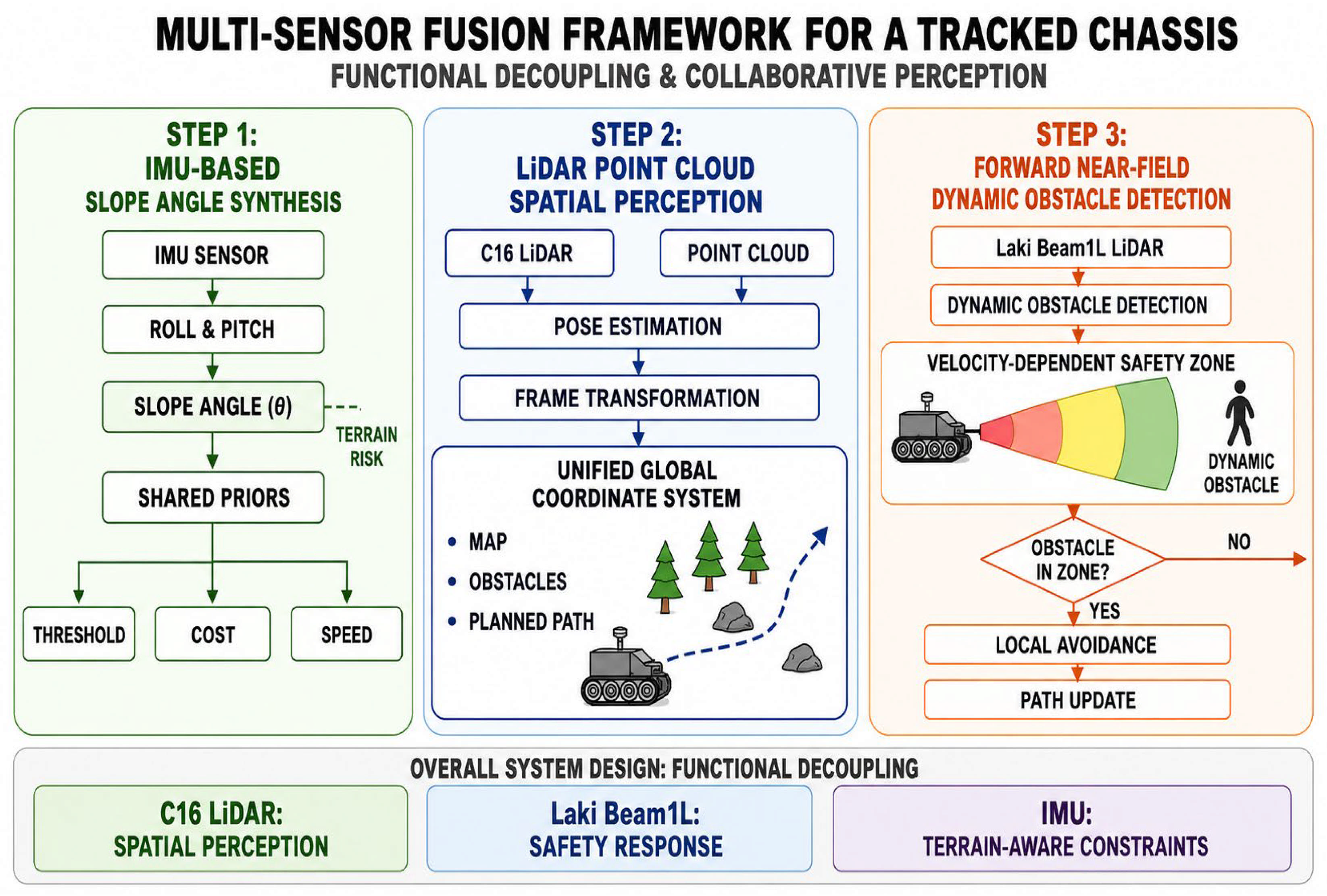
The proposed multi-sensor fusion framework adopts a function-decoupled fusion strategy. The IMU provides slope and attitude priors for terrain perception, the Leishen C16 mechanical LiDAR provides geometric information for mapping, localization, and obstacle representation, and the LakiBeam1L single-line LiDAR provides fast near-field safety triggering for dynamic obstacles. These sensors are not simply combined at the data level; instead, they are embedded into different stages of perception, localization, planning, and control according to their functional characteristics. Specifically, the IMU provides slope information for ground-segmentation threshold adjustment, path cost modeling, and velocity regulation; the Leishen C16 mechanical LiDAR provides point cloud constraints for pose estimation and obstacle representation; and the LakiBeam1L single-line LiDAR provides high-priority near-field risk signals for dynamic obstacle response. The sensor functions and information flow are illustrated in Figure 5.
In this framework, the IMU outputs roll, pitch, and heading angles. The roll and pitch angles are used to estimate the slope state of the chassis and are further incorporated into the ground-segmentation threshold, the slope–cross-slope joint path cost, and the velocity-adaptive control strategy. The heading angle is used to assist point cloud coordinate transformation and to provide the initial pose for NDT matching. The Leishen C16 mechanical LiDAR acquires three-dimensional environmental point clouds and transforms them into the world coordinate system, providing geometric information for NDT scan-to-map localization, Ray Ground Filter-based ground segmentation, Euclidean Cluster-based obstacle extraction, and path planning. The LakiBeam1L single-line LiDAR monitors the forward near-field region of the tracked agricultural chassis. When a dynamic obstacle enters the velocity-dependent safety zone, the system triggers deceleration, stopping, or local re-planning.
The point clouds acquired by the Leishen C16 mechanical LiDAR are initially expressed in the LiDAR coordinate system. To unify point clouds, maps, obstacles, and planned paths in the same coordinate system, the local point clouds are transformed into the world coordinate system using the estimated chassis pose. In hilly farmland, roll and pitch angles change the spatial relationship between the LiDAR point clouds and the ground surface. Therefore, the IMU attitude information is first used for point cloud attitude compensation, after which the compensated point clouds are projected into the world coordinate system. Let p i l denote the i -th point in the LiDAR coordinate system and p i w denote the corresponding point in the world coordinate system. The coordinate transformation is expressed as
p i w = R z ( ψ ) R y ( θ ) R x ( ϕ ) p i l + t ,
where ϕ , θ , and ψ are the roll, pitch, and heading angles measured by the IMU, respectively; R x ( ϕ ) , R y ( θ ) , and R z ( ψ ) are the rotation matrices around the x -, y -, and z -axes, respectively; and t is the translation vector from the LiDAR coordinate system to the world coordinate system. Through this transformation, local point clouds are mapped into a unified world coordinate system, providing the basis for subsequent NDT localization, obstacle-distance calculation, and path planning.
The roll angle ϕ and pitch angle θ measured by the IMU are further combined to estimate the equivalent terrain slope angle:
α i m u = a r c t a n t a n 2 ϕ + t a n 2 θ ,
where α i m u is the equivalent slope angle estimated from the IMU. This slope angle is not used as an independent control variable. Instead, it serves as a terrain-risk prior and is introduced into three key modules. First, it is used in ground segmentation to adaptively adjust the ground continuity threshold of the Ray Ground Filter. Second, it is used in global path planning to construct slope risk and cross-slope risk costs. Third, it is used in path tracking to regulate the linear velocity. In this way, IMU information is transformed from a pure attitude measurement into a unified terrain prior that affects perception, planning, and control.
The LakiBeam1L single-line LiDAR is not used for global mapping. Its primary function is to improve the response speed to forward near-field dynamic obstacles. The Leishen C16 mechanical LiDAR is responsible for spatial geometric modeling and obstacle representation, whereas the LakiBeam1L single-line LiDAR provides high-priority safety triggering in the near-field region. This design avoids relying exclusively on three-dimensional point cloud clustering for all safety decisions and provides a more direct deceleration or local avoidance signal when a dynamic obstacle rapidly approaches the tracked agricultural chassis.
A practical reason for retaining the LakiBeam1L single-line LiDAR as an independent safety sensor is that the Leishen C16 point cloud is optimized for spatial geometry reconstruction, mapping, and clustering rather than for deterministic millisecond-level emergency triggering. Using the C16 as the only near-field safety channel would couple emergency braking decisions to higher-dimensional point cloud processing and clustering latency. In contrast, the LakiBeam1L sensor provides a simple forward-sector decision rule based on distance and bearing, thereby forming an auxiliary but high-priority safety layer that can decelerate the chassis or trigger local re-planning even when the geometric point cloud pipeline is still being updated.
To make the system-level logic explicit, Table 3 links the IMU-derived information to the corresponding algorithm modules and evaluation metrics. This table is intended to prevent the reader from having to reconstruct the full logic from separated module descriptions.

2.4. Localization, Segmentation, Planning, and Control

2.4.1. IMU-Aided NDT Localization on Sloped Terrain

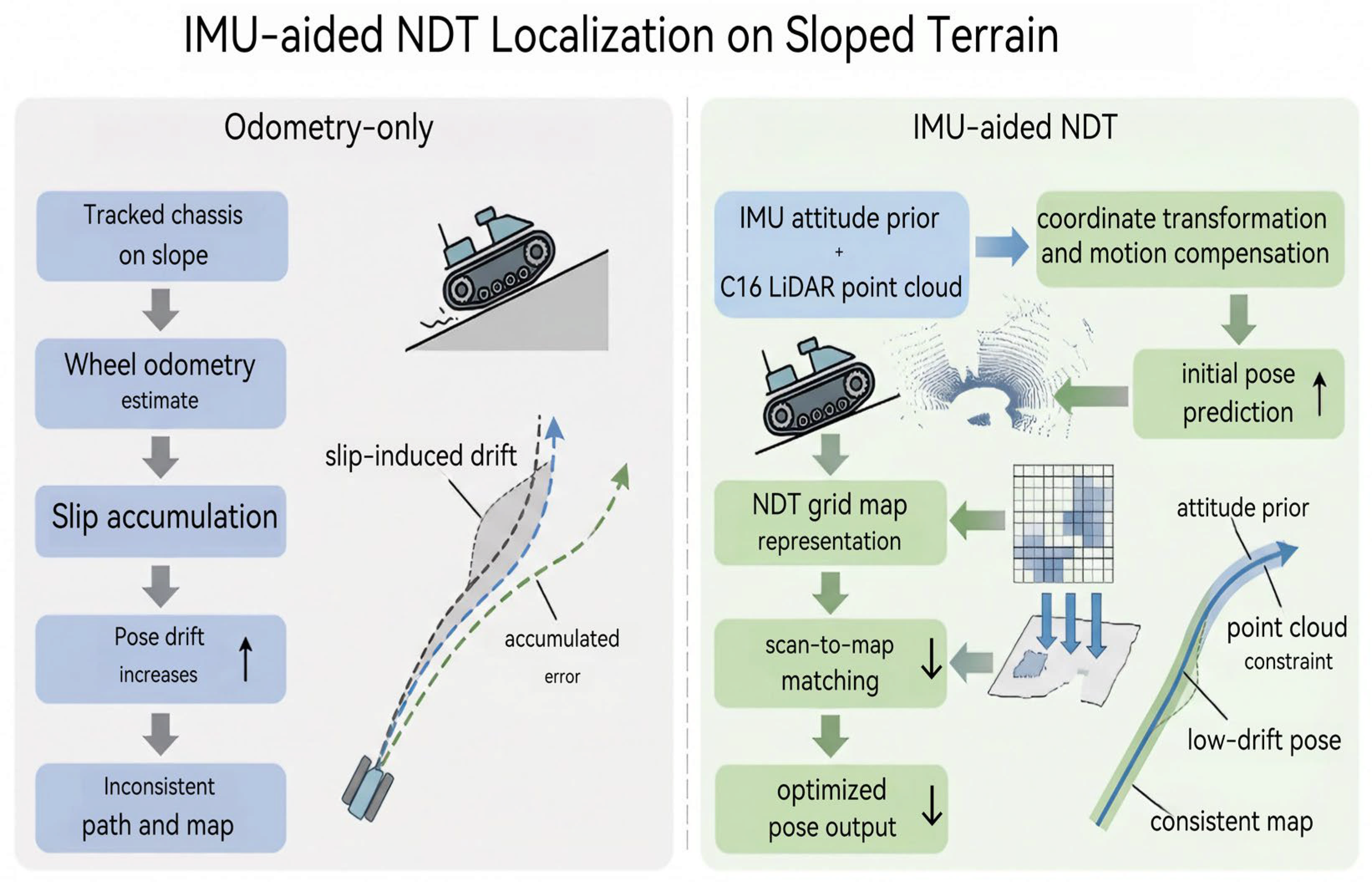
Tracked agricultural chassis are prone to slip when operating on sloped terrain, and relying solely on odometry may lead to accumulated pose errors. To mitigate this problem, this study adopts the Normal Distributions Transform (NDT) method for point cloud map construction and localization, while using IMU-derived attitude priors to enhance localization stability under hilly farmland conditions. Figure 6 shows the proposed IMU-aided NDT localization process. Compared with localization based only on odometry, the proposed method uses IMU attitude information to constrain the point cloud transformation and then performs NDT scan-to-map matching to evaluate the consistency between the current scan and the map distribution, thereby obtaining a corrected pose estimate.
It should be noted that the IMU prior in this study is introduced as a direct initial-pose constraint rather than as an additional regularization term in the NDT objective function. Specifically, the IMU contributes to NDT localization in two aspects. First, roll and pitch information are used to compensate the current point cloud before NDT matching, so that sloped-ground point clouds are represented in a more consistent spatial relationship. Second, the IMU heading angle is combined with the odometry-based translational prediction to form the initial pose for NDT scan-to-map matching. This reduces the search range and improves matching convergence. The optimization objective of NDT remains the consistency between the current point cloud and the probability distribution of the map grids.
Let x k o d o m y k o d o m be the planar position predicted by odometry at time step k , and let ψ k i m u be the heading angle measured by the IMU. The initial pose for NDT matching is defined as
q k 0 = [ x k o d o m , y k o d o m , ψ k i m u ] T ,
where q k 0 is the initial pose for NDT scan-to-map matching. If the IMU heading angle contains short-term fluctuations, the initial heading can also be constructed using the optimized pose from the previous time step and the IMU heading increment, namely ψ k 0 = ψ k 1 + Δ ψ k i m u . Therefore, the IMU prior does not replace the final NDT localization result; rather, it provides a more reliable initial state for NDT optimization. The final pose is still determined by point cloud-to-map matching.
During the mapping stage, the attitude-compensated and coordinate-transformed Leishen C16 point clouds are divided into two-dimensional or local three-dimensional grid cells. Each NDT grid stores the mean and covariance of the points within the cell. Suppose that the k -th grid contains n points. The mean and covariance are computed as
μ k = 1 n i = 1 n   p i ,
Σ k = 1 n 1 i = 1 n   ( p i μ k ) ( p i μ k ) T + λ I ,
where μ k is the point cloud mean of the k -th grid, Σ k is the covariance matrix, and λ I is a regularization term used to avoid covariance singularity. These grid-wise Gaussian distributions form a probabilistic map for subsequent scan-to-map matching.
During the localization stage, the current scan is projected under a candidate pose q , initialized by q k 0 , and the Mahalanobis distance between the transformed scan points and the corresponding NDT map grids is calculated. The NDT matching cost is defined as
J N D T ( q ) = 1 M i = 1 M   ( T ( q ) p i μ c ( i ) ) T Σ c ( i ) 1 ( T ( q ) p i μ c ( i ) ) ,
where M is the number of points in the current scan, T ( q ) is the point cloud transformation determined by the candidate pose q , c ( i ) is the index of the NDT grid containing the i -th transformed point, and μ c ( i ) and Σ c ( i ) are the mean and covariance of the corresponding grid, respectively. A smaller cost indicates better consistency between the current scan and the local probability distribution of the map.
The optimized pose at time step k is obtained as
q k = a r g m i n q Ω ( q k 0 )   J N D T ( q ) ,
where q k is the optimized pose, and Ω ( q k 0 ) is the local search space centered on the IMU–odometry initial pose q k 0 . Compared with NDT localization without prior information or NDT initialized only by odometry, the proposed method reduces the initial-pose deviation through IMU attitude constraints and decreases the probability of matching divergence or local misalignment under sloped-terrain slip conditions.
In summary, the proposed IMU-aided NDT localization process consists of four steps: obtaining translational prediction from odometry, compensating the Leishen C16 point cloud using IMU roll and pitch information, constructing the NDT initial pose using odometry and IMU heading, and optimizing the pose through scan-to-map matching. In this way, the localization problem caused by track slip on sloped terrain is converted into a consistency optimization problem between the current scan and the probabilistic point cloud map. This improves pose estimation stability for tracked agricultural chassis operating in hilly farmland.

2.4.2. Slope-Adaptive Ground Segmentation and Obstacle Clustering

For path planning of a tracked agricultural chassis, it is necessary to accurately distinguish traversable ground points from non-ground obstacle points. In hilly farmland, LiDAR point clouds contain ground points, obstacle points, and outliers caused by measurement noise. If the ground-segmentation threshold is too small, continuous sloped ground may be incorrectly classified as obstacles, reducing the available traversable space. Conversely, if the threshold is too large, low obstacles may be incorrectly classified as ground points, thereby reducing obstacle-avoidance safety. Therefore, the key challenge of ground segmentation on sloped terrain is to adaptively adjust the ground continuity criterion according to terrain slope variation.
In this study, the Ray Ground Filter algorithm is used for slope-adaptive ground segmentation. The algorithm organizes point clouds into radial rays according to their azimuth angles and determines whether each point belongs to the ground by evaluating the height continuity between adjacent points along the same ray. Different from the fixed-threshold strategy used in the baseline algorithm, the proposed method introduces the IMU-derived slope angle into the Ray Ground Filter, allowing the ground continuity threshold to vary with terrain slope.
Let x i y i denote the horizontal coordinates of the i -th point in the local point cloud. Its polar representation is given by
r i = x i 2 + y i 2 , β i = a t a n 2 ( y i , x i ) ,
where r i is the horizontal distance from the point to the LiDAR origin, and β i is the azimuth angle of the point. The point cloud is divided into multiple rays according to β i , and the points on each ray are sorted in ascending order of r i .
The baseline algorithm uses a fixed threshold for ground segmentation. This strategy can perform well on flat or slightly sloped terrain, but it is prone to misclassifying continuous sloped surfaces as obstacles under large-slope conditions. To address this problem, the proposed method constructs a slope-adaptive ground continuity threshold based on the IMU-derived slope angle:
τ g = t a n ( c l i p ( α i m u + Δ α , α m i n , α m a x ) ) ,
where τ g is the ground continuity threshold, α i m u is the equivalent slope angle estimated by the IMU, Δ α is the local terrain undulation margin used to compensate for surface unevenness and sensor noise, and α m i n and α m a x are the lower and upper bounds of the threshold, respectively. The clipping function prevents the segmentation from becoming overly strict when the estimated slope is too small and prevents low obstacles from being incorrectly merged into ground points when the estimated slope is too large.
It should be emphasized that the output of the clipping function in Equation (9) is an angle. After applying the tangent function, τ g becomes a dimensionless quantity. This quantity is not a height threshold in the conventional sense; rather, it represents the allowable ground-slope variation rate, namely the maximum allowable height variation per unit horizontal distance:
τ g Δ z a l l o w Δ r ,
Thus, τ g can be directly compared with the measured height variation rate between adjacent points. When the terrain slope increases, α i m u increases and τ g also increases, allowing larger height variation between adjacent ground points. This reduces the probability of misclassifying continuous sloped ground as obstacles. When the terrain is relatively flat, τ g remains small, maintaining a stricter ground continuity criterion and reducing the risk of classifying low obstacles as ground points.
Let z i be the height of the current point, z g be the height of the previous ground reference point, and r i and r g be their corresponding horizontal distances from the LiDAR origin. The ground-point judgment criterion is defined as
z i z g m a x ( r i r g , ε ) < τ g ,
where z i z g is the height difference between the current point and the previous ground reference point, m a x ( r i r g , ε ) is the effective horizontal distance between the two points, and ε is a small positive value used to avoid division by zero. The left-hand side of Equation (11) represents the measured height variation rate, while the right-hand side represents the allowable ground-slope variation rate determined by the IMU-derived slope prior. If the measured height variation rate is lower than τ g , the current point is classified as a ground point; otherwise, it is assigned to the non-ground point set and used as a candidate point for subsequent obstacle clustering.
Through Equations (9)–(11), the IMU-derived slope angle is converted from an attitude measurement into a geometric criterion for point cloud segmentation. This enables the Ray Ground Filter to adapt to slope changes instead of relying on a fixed empirical threshold. Compared with fixed-threshold segmentation, the proposed method is more suitable for hilly farmland with significant slope variation and can reduce false obstacles and loss of traversable space caused by slope-induced ground misclassification.
After ground segmentation, Euclidean clustering is applied to the non-ground point set to extract obstacle candidates. Points with spatial distances smaller than a specified clustering radius are grouped into the same obstacle cluster. Let C j denote the j -th cluster and N j be the number of points in this cluster. The cluster center is calculated as
c j = 1 N j i C j   p i ,
and the approximate cluster radius is defined as
ρ j = m a x i C j   p i c j ,
where c j is the center of the j -th obstacle cluster, ρ j is its approximate radius, and p i is the coordinate of a point in the cluster. The cluster center and radius are used for obstacle representation, obstacle inflation, safety clearance calculation, and perception accuracy evaluation. To reduce the influence of noise and isolated outliers, candidate clusters are further filtered according to point-number thresholds and radius constraints, removing clusters with too few points or abnormal sizes.
In summary, the proposed slope-adaptive point cloud processing procedure consists of four steps: organizing the attitude-compensated Leishen C16 point cloud into radial rays, calculating the allowable ground-slope variation rate using IMU-derived slope information, performing adaptive ground-point judgment along each ray, and applying Euclidean clustering to non-ground points. The role of this module is not simply to increase the number of detected clusters, but to improve the reliability of obstacle representation by reducing slope-induced ground misclassification. The resulting obstacle centers and radii provide more stable inputs for path cost calculation, obstacle inflation, dynamic safety clearance evaluation, and subsequent local avoidance.

2.4.3. Slope-Aware Path Planning and Dynamic Obstacle Avoidance

The baseline global path planner adopts the Dijkstra algorithm to search for the minimum-cost path from the start point to the target point in the grid map. In the baseline algorithm, only the Euclidean norm between adjacent grid nodes is used as the edge cost, which is defined as
c i j b a s i c = | | p i p j | | 2 ,
where c i j b a s i c is the edge cost from node i to node j in the baseline algorithm, and p i and p j are the position vectors of two adjacent grid nodes. The notation p i p j 2 denotes the Euclidean norm, and therefore c i j b a s i c has the physical unit of meters.
To address this limitation, a slope–cross-slope joint path cost model is constructed in this study. The proposed edge cost integrates path length, slope risk, cross-slope risk, and obstacle proximity, and is defined as
c i j = | | p i p j | | 2 1 + k s η 2 ( p j ) + k c χ ( p j , ψ ) + k o e x p d o b s ( p j ) σ ,
where c i j is the integrated edge cost from node i to node j , p i p j 2 is the Euclidean distance between adjacent grid nodes, η ( p j ) is the normalized slope risk function at node p j , and χ ( p j , ψ ) is the cross-slope risk function related to the chassis heading ψ . In addition, d o b s ( p j ) is the distance from node p j to the nearest obstacle boundary, k s , k c , and k o are dimensionless weighting coefficients, and σ is the attenuation parameter of the obstacle potential field.
The dimensional consistency of Equation (15) was explicitly checked. The Euclidean edge length p i p j 2 has units of meters. The bracketed factor is dimensionless because η ( p j ) , χ ( p j , ψ ) , and e x p [ d o b s ( p j ) / σ ] are dimensionless, while k s , k c , and k o are dimensionless weighting coefficients. The ratio d o b s ( p j ) / σ is dimensionless when σ is expressed in meters. Therefore, c i j retains the unit of equivalent path length in meters.
Slope risk function
Let α ( p j ) denote the local slope angle at node p j , and let α l i m denote the maximum safe slope angle of the chassis. The normalized slope risk function is defined as
η ( p j ) = c l i p α ( p j ) α l i m 0 1 ,
where α ( p j ) can be obtained from the IMU-derived slope estimate, the simulated slope map, or the local terrain height difference. The parameter α l i m represents the safe slope limit of the tracked agricultural chassis. In this study, the maximum climbing capability of the chassis is no more than 30 ° ; therefore, α l i m = 30 ° is used in the simulation. The value of η ( p j ) ranges from 0 to 1. A smaller local slope corresponds to a lower slope risk, whereas a local slope approaching the safe slope limit corresponds to a higher slope risk.
In Equation (15), η ( p j ) 2 is used instead of η ( p j ) to enhance the penalty for high-slope regions. For mild slopes, the quadratic term increases slowly and avoids excessive sensitivity to slight terrain variation. For steep slopes, the quadratic term increases more rapidly, encouraging the planner to avoid high-risk slope regions. This design follows the engineering principle that low-slope areas are generally passable, whereas high-slope areas should be treated more conservatively.
Cross-slope risk function
Considering only the slope magnitude is insufficient to characterize the driving risk of a tracked agricultural chassis on sloped terrain. For the same slope surface, the main risk during uphill or downhill motion is longitudinal slip, whereas lateral sideslip and rollover risk increase when the chassis moves across the slope. Therefore, a heading-related cross-slope risk function is further introduced.
Let ψ s ( p j ) denote the steepest downslope direction of the local terrain at node p j , and let ψ denote the current or planned motion direction of the chassis. The angular difference between these two directions is defined as
Δ ψ j = w r a p ψ ψ s ( p j ) ,
where w r a p ( ) normalizes the angle to the range π , π . When the motion direction is parallel or anti-parallel to the steepest downslope direction, the chassis mainly moves uphill or downhill. When the motion direction is approximately perpendicular to the steepest downslope direction, the chassis moves across the slope. Based on this relationship, the cross-slope risk function is defined as
χ ( p j , ψ ) = η 2 ( p j ) s i n 2 ( Δ ψ j ) ,
where s i n 2 ( Δ ψ j ) describes the lateral component of the chassis motion relative to the slope direction. When Δ ψ j 0 or π , the chassis moves along the slope direction and the cross-slope risk is relatively low. When Δ ψ j π / 2 , the chassis moves across the slope, and s i n 2 ( Δ ψ j ) approaches 1, resulting in a high cross-slope risk. Multiplying this term by η ( p j ) 2 ensures that cross-slope risk is jointly determined by slope magnitude and motion direction. On flat terrain, cross-slope risk remains low even if the motion direction is perpendicular to the slope direction; on steep terrain, cross-slope motion is strongly penalized.
In a two-dimensional grid simulation, if the slope direction is known, ψ s ( p j ) can be directly assigned according to the simulated terrain. If a terrain height map is available, the steepest downslope direction can be calculated from the local height gradient as
ψ s ( p j ) = a t a n 2 z y , z x ,
where z / x and z / y are the terrain height gradients in the x and y directions, respectively. The negative gradient direction represents the steepest downhill direction of the local terrain.
Obstacle potential term
In addition to slope and cross-slope risks, the planned path should maintain a sufficient distance from obstacle boundaries to account for chassis width, perception uncertainty, and tracking errors. Therefore, an exponential obstacle potential term is used to represent the near-field risk of obstacles:
Φ o b s ( p j ) = e x p d o b s ( p j ) σ ,
where Φ o b s ( p j ) is the obstacle potential cost, d o b s ( p j ) is the distance from node p j to the nearest obstacle boundary, and σ is the attenuation parameter. The obstacle potential cost is high when the node is close to an obstacle and decreases rapidly as the distance increases. The exponential function is used because obstacle-related risk has a strong near-field characteristic: strong penalties should be imposed near obstacle boundaries, while distant obstacles should not excessively influence the path search. The weighted obstacle potential contribution in Equation (15) is k o Φ o b s ( p j ) .
Accordingly, Equation (15) can be interpreted as a combination of four factors. The first term, p i p j , prevents unnecessary path-length increase. The slope risk term k s η ( p j ) 2 encourages the path to avoid steep regions. The cross-slope risk term k c χ ( p j , ψ ) suppresses cross-slope motion under high-slope conditions. The obstacle potential term Φ o b s ( p j ) encourages the path to maintain a safe distance from obstacle boundaries. Compared with the baseline algorithm that only considers geometric distance, the proposed cost model explicitly introduces terrain traversability and obstacle safety into the edge cost, making the planned path more suitable for execution by a tracked agricultural chassis in hilly farmland.
The cumulative-cost update of the Dijkstra algorithm is expressed as
g ( j ) = m i n i N ( j )   [ g ( i ) + c i j ] ,
where g ( j ) is the minimum cumulative cost from the start point to node j , N ( j ) is the set of neighboring nodes of j , and c i j is the integrated edge cost calculated using Equation (15). Through Equations (14)–(21), the planner considers not only path length but also slope safety, cross-slope risk, and obstacle proximity during path search.
Local re-planning for dynamic obstacle avoidance
The global planner mainly handles static obstacles and terrain-related risk. However, dynamic obstacles may suddenly enter the planned path and require a faster safety response. To improve the response capability under dynamic obstacle scenarios, a local A* re-planning strategy is introduced on the basis of the global path. When the LakiBeam1L single-line LiDAR detects that a dynamic obstacle has entered the forward safety zone, a local grid window is constructed around the current chassis position, and the dynamic obstacle is inflated according to the chassis size and safety margin.
The evaluation function of the local A* planner is defined as
f ( n ) = g ( n ) + h ( n ) , h ( n ) = p n p g o a l l o c a l ,
where f ( n ) is the evaluation value of node n , g ( n ) is the cumulative cost from the local start point to node n , and h ( n ) is the heuristic distance from node n to the local target point p g o a l l o c a l . The local target point is usually selected as a reference point on the global path ahead of the current chassis position, so that the chassis can return to the global path after avoiding the dynamic obstacle.
The inflated dynamic obstacle region is defined as
p p d y n r d y n + r b + m d y n ,
where p is the grid point to be evaluated, p d y n is the position of the dynamic obstacle, r d y n is the dynamic obstacle radius, r b is the equivalent safety radius of the chassis, and m d y n is the dynamic safety margin. Grid cells satisfying Equation (23) are regarded as dynamically non-traversable regions. This inflation process accounts for obstacle size, chassis envelope, and dynamic avoidance margin, preventing the local path from passing too close to the dynamic obstacle.
The local obstacle-avoidance process is as follows. First, the LakiBeam1L LiDAR determines whether a forward dynamic obstacle has entered the velocity-dependent safety zone. If the trigger condition is satisfied, the local cost map is updated by inflating the dynamic obstacle within the local grid window. Then, the local A* planner searches for a temporary avoidance path in the updated local cost map. After bypassing the obstacle, the chassis returns to the original global path when the safety condition is restored. If no feasible local path exists within the local window, the chassis executes deceleration or stopping to ensure safety.

2.4.4. Slope-Adaptive Path Tracking and Near-Field Safety Control

This study adopts the Pure Pursuit algorithm for path tracking and introduces a slope-adaptive velocity regulation mechanism in the proposed method. Pure Pursuit selects a look-ahead target point on the reference path according to the current chassis position and the look-ahead distance, and then calculates the desired curvature based on the target point angle. In the proposed method, slope and heading error factors are further incorporated into the velocity command. Specifically, the linear velocity is reduced when the terrain slope increases or when the steering demand becomes larger. This strategy aims to reduce sideslip and trajectory oscillation during turning on sloped terrain. In addition, when the LakiBeam1L single-line LiDAR detects a dynamic obstacle risk, the system further constrains the velocity and triggers local re-planning.
Let L d denote the look-ahead distance, v denote the current linear velocity of the chassis, L 0 denote the basic look-ahead distance, and k v denote the velocity gain. The look-ahead distance is defined as
L d = L 0 + k v v ,
Let γ denote the angle of the look-ahead target point in the chassis coordinate system. The desired curvature of Pure Pursuit is calculated as
κ = 2 s i n   γ L d ,
where κ is the desired path-tracking curvature, and γ is the angle between the look-ahead target point and the current heading direction of the chassis. A larger target point angle indicates a higher steering demand and therefore a larger desired curvature.
To reduce the risk of sideslip and tracking oscillation on sloped terrain, a slope-related velocity ratio s α is defined as
s α = c l i p 1 1 s m i n α i m u α 0 α l i m α 0 , s m i n , 1 ,
where s α is the slope-related velocity ratio, α i m u is the slope angle estimated by the IMU, α 0 is the slope threshold at which velocity reduction begins, α l i m is the safe slope limit of the chassis, and s m i n is the minimum allowable velocity ratio near the maximum slope. The clipping function constrains the velocity ratio within a reasonable range.
In this study, the maximum climbing capability of the tracked agricultural chassis is no more than 30 ° ; therefore, α l i m = 30 ° is adopted. Considering that the chassis can still maintain relatively stable motion on mild slopes, α 0 = 5 ° is used as the initial slope threshold for velocity reduction. To avoid excessive speed on steep slopes, which may cause sideslip and tracking oscillation, s m i n = 0.45 is used. According to Equation (26), when α i m u 5 ° , s α = 1 , and the chassis maintains the normal tracking velocity. As α i m u approaches 30 ° , s α gradually decreases and is finally limited by s m i n . Thus, the slope-related velocity ratio is determined by the chassis slope capability and the minimum safe velocity ratio, rather than by an arbitrary empirical coefficient.
In addition to slope, steering demand also affects the stability of a tracked agricultural chassis on sloped terrain. When the chassis turns sharply on a slope, a large look-ahead target angle may increase the risk of lateral slip and trajectory oscillation. Therefore, a heading error-related velocity ratio is defined as
s γ = c l i p ( 1 k γ γ , s γ , m i n , 1 ) ,
where s γ is the heading error-related velocity ratio, k γ is the heading error velocity regulation coefficient, and s γ , m i n is the minimum allowable velocity ratio under heading error constraints. This equation indicates that a larger target point angle leads to a lower linear velocity, thereby reducing the risk of sideslip during sharp turning on sloped terrain.
The linear and angular velocity commands are defined as
v c m d = c l i p ( v m a x s α s γ , v m i n , v m a x ) ,
ω c m d = c l i p ( v c m d κ , ω m a x , ω m a x ) ,
where v c m d and ω c m d are the commanded linear and angular velocities, respectively; v m a x and v m i n are the maximum and minimum linear velocities; and ω m a x is the maximum angular velocity. Equations (26)–(29) show that the controller jointly regulates the linear velocity using the slope factor and the heading error factor, and then calculates the angular velocity according to the desired curvature. The design principle is to reduce the linear velocity when the slope is steep or the path curvature is large, thereby decreasing sideslip and oscillation during slope traversal and turning. When the slope is mild and the path is relatively smooth, the chassis maintains a higher velocity to avoid overly conservative motion. This control law is an engineering-oriented strategy for sloped agricultural scenarios, and its effectiveness is evaluated through system-level simulations in this study.
Meanwhile, the LakiBeam1L single-line LiDAR is used for forward near-field dynamic obstacle safety detection. Let D denote the relative distance between the dynamic obstacle and the chassis center, and let β denote the relative bearing angle of the dynamic obstacle with respect to the chassis heading. They are calculated as
D = p d y n p r o b o t ,
β = w r a p [ a t a n 2 ( y d y n y r o b o t , x d y n x r o b o t ) ψ ] ,
where p r o b o t is the chassis position, p d y n is the dynamic obstacle position, and ψ is the heading angle of the chassis. The value D represents the distance between the dynamic obstacle and the chassis center, while β represents the obstacle bearing relative to the forward direction of the chassis.
To account for the influence of motion velocity on braking distance and avoidance distance, a velocity-dependent safety distance is defined as
D s a f e = D 0 + T r m a x ( v c m d , 0 ) + v c m d 2 2 a d e c + r b + r d y n ,
where D 0 is the basic safety distance, T r is the perception and control response time, a d e c is the allowable deceleration, r b is the equivalent safety radius of the chassis, and r d y n is the equivalent radius of the dynamic obstacle. Equation (32) consists of the basic safety distance, the distance traveled during the response time, the braking distance, and the geometric safety radii. Therefore, it explicitly reflects the fact that a higher velocity requires a larger safety distance.
The dynamic obstacle triggering condition is defined as
| β | β m a x , D D s a f e ,
where β m a x is the half-angle of the forward detection sector. When Equation (33) is satisfied, the dynamic obstacle is considered to have entered the forward safety zone of the chassis, and the system switches to the near-field safety control mode.
Under the near-field safety control mode, the system first reduces the velocity command and triggers local re-planning if a feasible avoidance path exists. If the obstacle continues to approach and the remaining distance is insufficient for safe avoidance, the chassis executes a stopping command. In this way, conventional path tracking and near-field safety intervention are handled in a hierarchical manner: Pure Pursuit provides the reference tracking command, slope-adaptive velocity regulation reduces terrain-induced motion risk, and the LakiBeam1L-based safety trigger provides high-priority intervention for dynamic obstacles.
In summary, the proposed path-tracking and safety control procedure consists of four steps: selecting a look-ahead target point and calculating the desired curvature, computing the slope-related and heading error-related velocity ratios, generating the constrained linear and angular velocity commands, and applying near-field safety intervention when a dynamic obstacle enters the velocity-dependent safety zone. The purpose of this control strategy is not to minimize travel time, but to improve trajectory stability and dynamic safety clearance for tracked agricultural chassis operating under hilly farmland conditions.


2.5. Simulation Implementation and Evaluation Metrics

To comprehensively evaluate the performance of the baseline and proposed algorithms, this study used several metrics, including actual path length, tracking root mean square error (RMSE), localization RMSE, static safety clearance, dynamic safety clearance, obstacle recall, and clustering precision. These metrics were used to evaluate the two algorithms in terms of path execution, localization accuracy, obstacle-avoidance safety, and perception performance.
The actual path length is defined as the cumulative distance between adjacent trajectory sampling points:
L = t = 1 T 1   p t + 1 p t ,
where L is the actual path length, p t is the chassis position at time step t , and T is the total number of trajectory sampling points. This metric reflects the actual travel distance of the tracked agricultural chassis.
The tracking RMSE is used to evaluate the deviation of the actual trajectory from the reference path:
R M S E t r a c k = 1 T t = 1 T   d i s t ( p t , P r e f ) 2 ,
where P r e f is the reference path, and d i s t ( p t , P r e f ) is the shortest distance from the chassis position p t to the reference path. A smaller tracking RMSE indicates better path-tracking performance.
The localization RMSE is used to evaluate the difference between the estimated pose and the ground-truth pose in simulation:
R M S E l o c = 1 T t = 1 T   p t p ^ t 2 ,
where p t is the ground-truth position provided by the simulation environment, and p ^ t is the estimated position output by the localization algorithm. A smaller localization RMSE indicates higher localization accuracy and stability.
The static safety clearance is calculated as the minimum distance between the chassis trajectory and the boundaries of static obstacles:
D s t a t i c = m i n t , j   p t o j r b r j ,
where o j is the center of the j -th static obstacle, r j is the obstacle radius, and r b is the equivalent safety radius of the chassis. A larger static safety clearance indicates a greater safety margin between the chassis and static obstacles.
The dynamic safety clearance is calculated as the minimum distance between the chassis trajectory and the boundary of the dynamic obstacle:
D d y n = m i n t   p t o d y n ( t ) r b r d y n ,
where o d y n ( t ) is the position of the dynamic obstacle at time step t , and r d y n is the equivalent radius of the dynamic obstacle. A larger dynamic safety clearance indicates a greater safety margin during dynamic obstacle avoidance. If D d y n < 0 , a geometric overlap occurs between the chassis and the dynamic obstacle, which is regarded as a collision or unsafe contact.
Obstacle recall is used to evaluate the proportion of true obstacles that are correctly detected:
R o b s = N T P N T P + N F N × 100 % ,
Clustering precision is used to evaluate the proportion of detected obstacle clusters that correspond to true obstacles:
P c l u s t e r = N T P N T P + N F P × 100 % ,
where N T P is the number of correctly detected obstacles, N F N is the number of missed obstacles, and N F P is the number of false obstacle detections. Higher obstacle recall indicates fewer missed obstacles, whereas higher clustering precision indicates fewer false obstacle clusters.
For error-type metrics, such as tracking RMSE and localization RMSE, a lower value indicates better performance. The reduction rate is defined as
I m = M b a s i c M p r o p o s e d M b a s i c × 100 % ,
For positive metrics, such as safety clearance, obstacle recall, and clustering precision, a higher value indicates better performance. The improvement rate is defined as
I m + = M p r o p o s e d M b a s i c M b a s i c × 100 % ,
where M b a s i c and M p r o p o s e d are the values of the baseline algorithm and the proposed algorithm under the same metric and scenario, respectively. I m denotes the reduction rate of error-type metrics, and I m + denotes the improvement rate of positive metrics. This evaluation system enables a systematic comparison of the two algorithms in terms of localization, tracking, obstacle avoidance, and perception.

2.5.1. Parameter Settings

Table 4 lists the key parameters used in the perception, planning, and control modules. These parameters were not determined by a single theoretical formula. Instead, they were selected through staged empirical tuning under the constraints of chassis capability, sensor characteristics, path safety, and tracking stability. First, preliminary tuning was conducted in the simple environment to ensure basic reachability and stable tracking. Then, the parameters were cross-validated in the general and complex environments, with emphasis on balancing path safety clearance, local avoidance behavior, trajectory smoothness, and control stability. Finally, a unified set of parameters that maintained consistent performance across the three environments was selected. The same parameter set was used for both the baseline and proposed algorithms, except for the parameters associated with the modules introduced only in the proposed method.
The parameters k s , k c , k o , and σ mainly affect global path planning. The parameters α l i m , α 0 , and s m i n determine the slope-adaptive velocity regulation strategy. The parameters L 0 , k v , k γ , v m a x , v m i n , and ω m a x mainly affect the stability of Pure Pursuit path tracking. The parameters D 0 , T r , a d e c , r b , r d y n , m d y n , and β m a x mainly affect dynamic obstacle near-field safety triggering. The parameters Δ α , α m i n , α m a x , and ε are associated with slope-adaptive ground segmentation. By distinguishing the functional roles of these parameters, the parameter design can be more clearly related to the corresponding algorithm modules and can be further recalibrated in future field experiments according to actual chassis dimensions, sensor installation positions, terrain conditions, and operating speeds.

2.5.2. Statistical Validation and Robustness Testing Protocol

To strengthen the reliability of the simulation evaluation, three supplementary validation protocols were introduced on top of the original Python and ROS/Gazebo simulations. First, each environment-slope-algorithm combination in the Python simulation was repeated 10 times using independent random seeds. To ensure reproducibility and paired comparison fairness, the random seeds used in the repeated trials were labeled as Seed 202501, Seed 202502, …, Seed 202510. For each environment–slope combination, the baseline and proposed algorithms used the same seed list, so that LiDAR noise, IMU perturbation, odometry-drift realization, and dynamic obstacle disturbance were generated under matched stochastic conditions. Therefore, the reported differences between the baseline and proposed algorithms were not caused by different random perturbation samples, but by the different algorithmic modules activated in each method. These seeds affected LiDAR noise, IMU perturbations, and odometry-drift realizations, yielding 150 records for each algorithm. Mean values, standard deviations, and 95% confidence intervals were calculated for the repeated-trial dataset. Second, the robustness of the IMU-derived slope prior was evaluated under nominal noise, vibration, drift, and combined dynamic-motion perturbations. Third, a one-at-a-time sensitivity analysis was performed for the planning parameters k s , k c , k o , and σ , while the remaining parameters were fixed at their nominal values.
The repeated-trial protocol was used to clarify the basis of the reported percentage improvements. For each metric, the baseline and proposed values were compared under the same case definition. Equation (41) was used for error-type metrics, and Equation (42) was used for positive metrics. The supplementary tables in Section 3.3 report the underlying mean values, standard deviations, confidence intervals, and sample counts, rather than only relative improvement rates. The dimensional consistency of the path cost function was verified in Section 2.4.3.
The nominal sensor noise model used in the Python simulation was as follows: IMU roll and pitch noise were modeled as zero-mean Gaussian noise with a standard deviation of 0.25°, yaw noise as 0.35°, gyroscope-z noise as 0.2°/s, accelerometer noise as 0.035 m/s2, and magnetometer-yaw noise as 0.8°. The C16 point cloud included 0.025 m local horizontal noise and approximately 0.025 m height noise. In the stress tests, additional IMU and C16 noise was superimposed. IMU drift was represented by a bounded random-walk bias, and vibration was represented by sinusoidal roll/pitch perturbations plus Gaussian noise. The current study did not implement a hardware vibration filter; instead, the adaptive threshold used a 7° terrain undulation allowance and a bounded threshold to reduce sensitivity to short-term slope estimation errors.
All baseline and proposed runs used the same map size, grid resolution, robot safety radius, maximum velocity, maximum yaw rate, sensor noise model, obstacle layouts, and start/goal definitions within each case. Parameters were not adjusted separately for individual slopes or environments. The baseline used its corresponding fixed-threshold Ray Ground Filter, distance cost Dijkstra planner, odometry localization, and conventional Pure Pursuit settings; the proposed method activated only the additional modules listed in the Materials and Methods Section. Thus, the comparison used a unified parameter set across all cases, while algorithm-specific parameters were enabled only when the corresponding module existed.

3. Results

3.1. Python Simulation Results

A Python simulation was used to provide a complete statistical comparison under three environmental types and five slope conditions. The simple environment contained three static circular obstacles and one dynamic obstacle; the general environment contained nine static circular obstacles and one dynamic obstacle; and the complex environment contained fifteen static circular obstacles and one dynamic obstacle. Each environment was tested under slope conditions of 5°, 10°, 15°, 20°, and 25°. The baseline and proposed algorithms were evaluated under the same environmental settings to obtain full comparative performance metrics.
To ensure a fair comparison, the baseline algorithm was implemented as a standard combination of fixed-threshold Ray Ground Filter, odometry-based localization, distance cost Dijkstra global planning, and conventional Pure Pursuit path tracking. The proposed algorithm introduced IMU-adaptive ground segmentation, IMU-aided NDT scan-to-map localization, slope–cross-slope joint path cost planning, local A* dynamic obstacle avoidance, and slope-adaptive velocity regulation. Both algorithms were compared using the same maps, obstacle layouts, start and goal positions, chassis dimensions, and evaluation metrics.
It should be noted that the baseline algorithm showed low arrival rates in some high-slope scenarios, even in the simple environment. This does not indicate that the baseline was intentionally weakened; rather, it reflects the fact that the baseline algorithm does not explicitly consider slope risk, track slip, dynamic obstacle safety zones, or slope-adaptive velocity regulation. As the slope increases, accumulated odometry error, fixed-speed tracking, and insufficient dynamic obstacle avoidance may lead to increased tracking deviation or safety constraint failure. Therefore, in the following analysis, both the original metric values and the relative improvement rates are reported to avoid overinterpretation based only on percentages.

3.1.1. Average Performance Metrics

As shown in Table 5, the proposed algorithm shows a stronger overall performance trend than the baseline algorithm across the three environments. This statement refers to the aggregate simulation-level trend and is interpreted together with the repeated-trial statistics and significance tests reported later.
In the complex environment, the baseline algorithm achieved an arrival rate of only 20.0% and a collision rate of 80.0%, whereas the proposed algorithm increased the arrival rate to 100.0% and reduced the collision rate to 0.0%. Meanwhile, the tracking RMSE decreased from 0.373 m to 0.180 m, the localization RMSE decreased from 0.425 m to 0.213 m, and the dynamic safety clearance increased from 1.214 m to 2.002 m. Obstacle recall and clustering precision increased from 79.35% and 82.83% to 98.51% and 98.66%, respectively.
In the general environment, the arrival rate increased from 40.0% to 100.0%, while the collision rate decreased from 60.0% to 0.0%. The tracking RMSE decreased from 0.379 m to 0.253 m, the localization RMSE decreased from 0.501 m to 0.251 m, and the dynamic safety clearance increased from 0.471 m to 1.683 m.
In the simple environment, although the obstacle constraints were weaker, the proposed algorithm still reduced the tracking RMSE from 0.922 m to 0.221 m and the localization RMSE from 1.052 m to 0.376 m. The dynamic safety clearance increased from 2.500 m to 3.237 m.
Table 6 further quantifies the performance changes of the proposed algorithm relative to the baseline algorithm. In the complex environment, the tracking RMSE, localization RMSE, and dynamic safety clearance improved by 51.74%, 49.88%, and 64.91%, respectively. In the general environment, the dynamic safety clearance showed the largest relative improvement, reaching 257.32%. This large percentage was mainly caused by the relatively low baseline value of 0.471 m; therefore, the absolute increase of 1.212 m should also be considered when interpreting this result. In the simple environment, the tracking RMSE, localization RMSE, and clustering precision improved by 76.03%, 64.26%, and 53.28%, respectively.
The simulation results in Table 5 and Table 6 demonstrate that the improvements in the enhanced algorithm are not confined to a single module; advancements have been achieved across multiple levels, including perception, localization, planning, and control.

3.1.2. Trends of Core Metrics with Slope

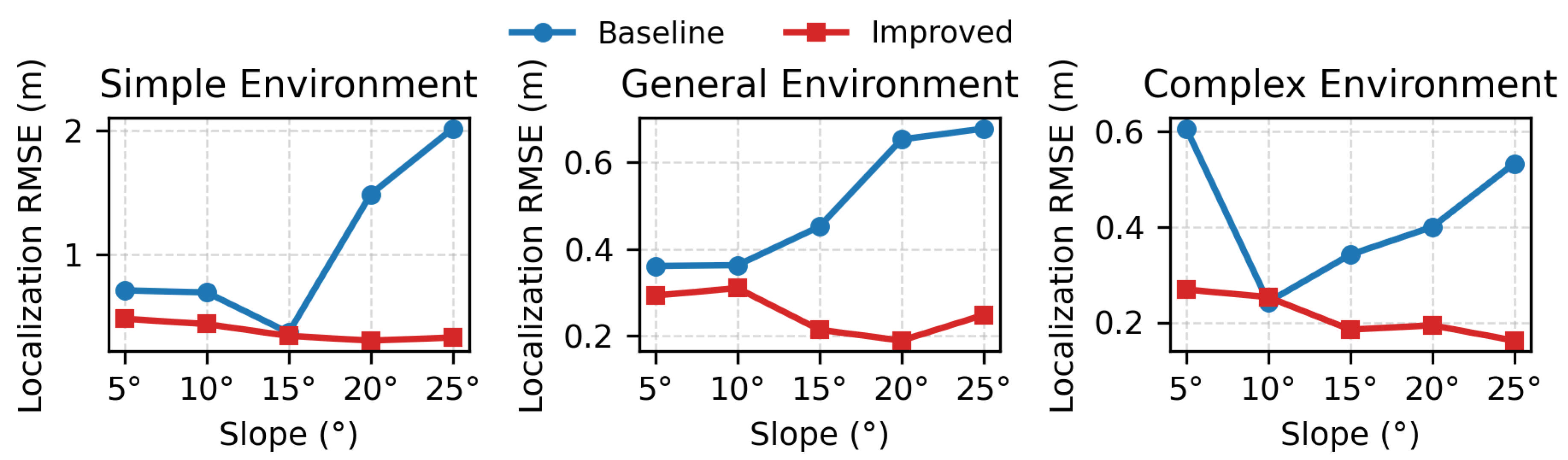
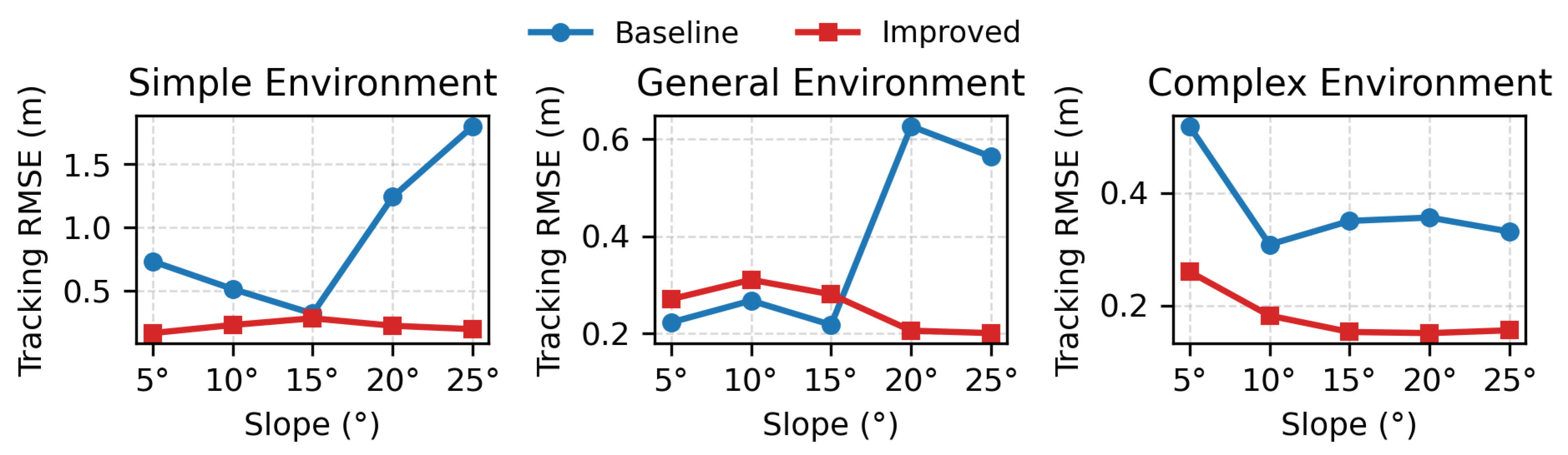
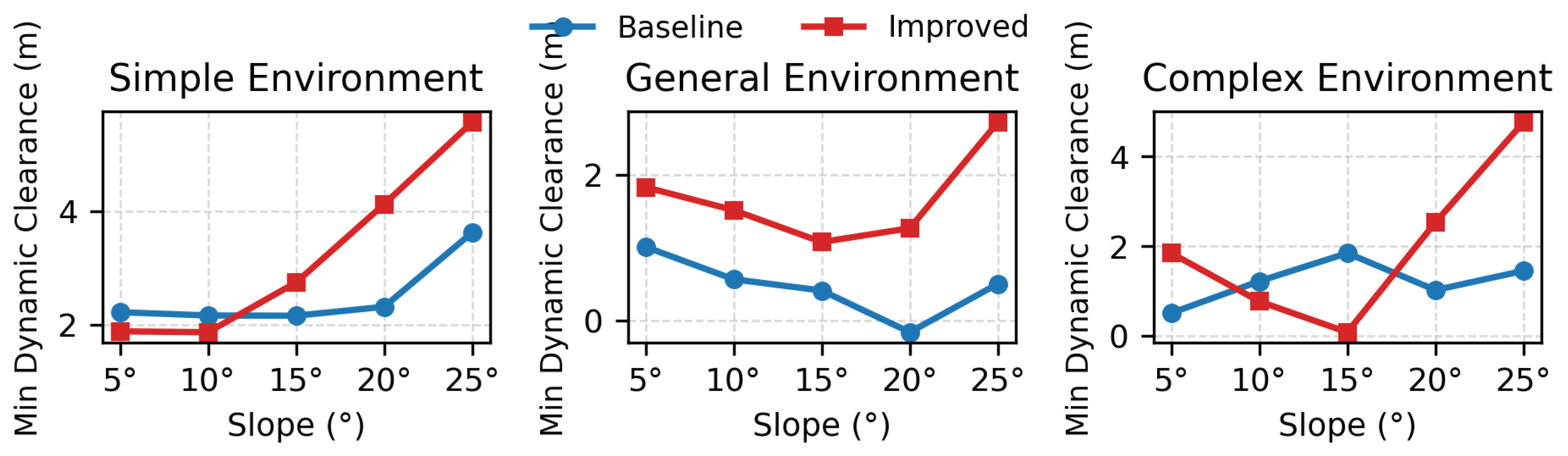
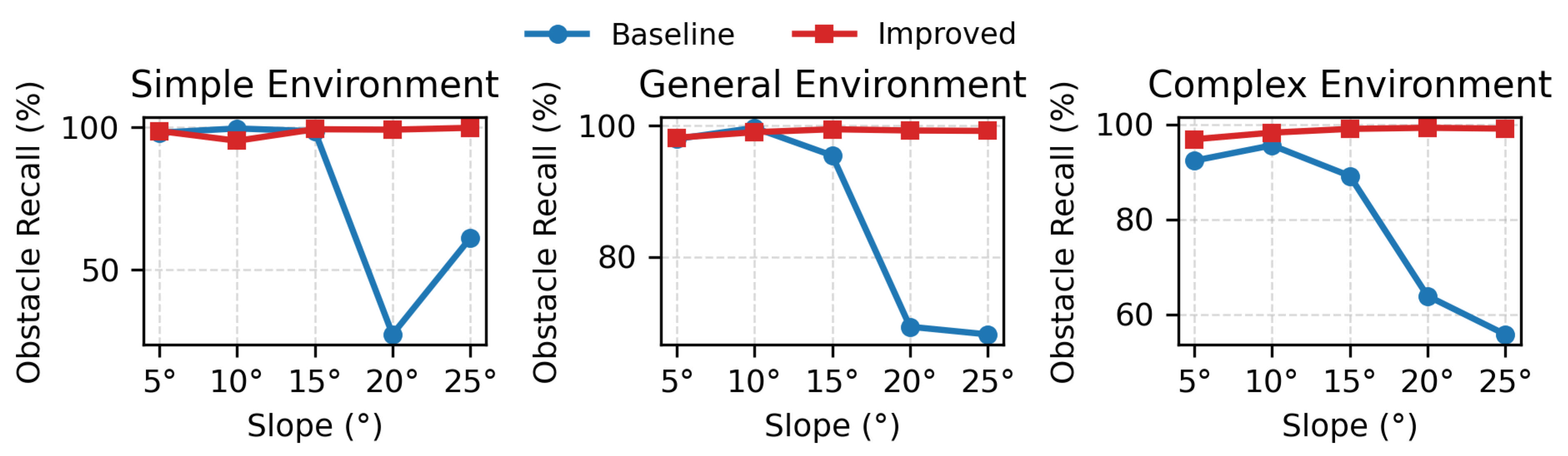
Figure 7, Figure 8, Figure 9 and Figure 10 show the original deterministic trend plots and are retained to illustrate how the metrics vary with slope. The statistical interpretation is based on the repeated-trial and mixed-perturbation analyses added in Section 3.3.1 and Section 3.3.5; therefore, the trend figures should be read as visual summaries rather than as standalone statistical evidence.
Figure 7 shows that the tracking RMSE of the baseline algorithm increased markedly after the slope exceeded 20°, whereas the proposed algorithm maintained a lower tracking error. This result indicates that slope-aware path cost and velocity regulation contributed to trajectory stability under high-slope conditions.
Figure 8 shows that the proposed algorithm achieved lower localization RMSE than the baseline algorithm in all three environments, especially under high-slope conditions. This suggests that NDT scan-to-map localization can reduce odometry drift caused by track slip on sloped terrain.
Figure 9 shows that the proposed algorithm maintained larger dynamic safety clearance in most scenarios. This improvement is attributed to the integration of the LakiBeam1L-based velocity-dependent safety zone and local A* re-planning, which enhanced the dynamic obstacle response, particularly in the general and complex environments.
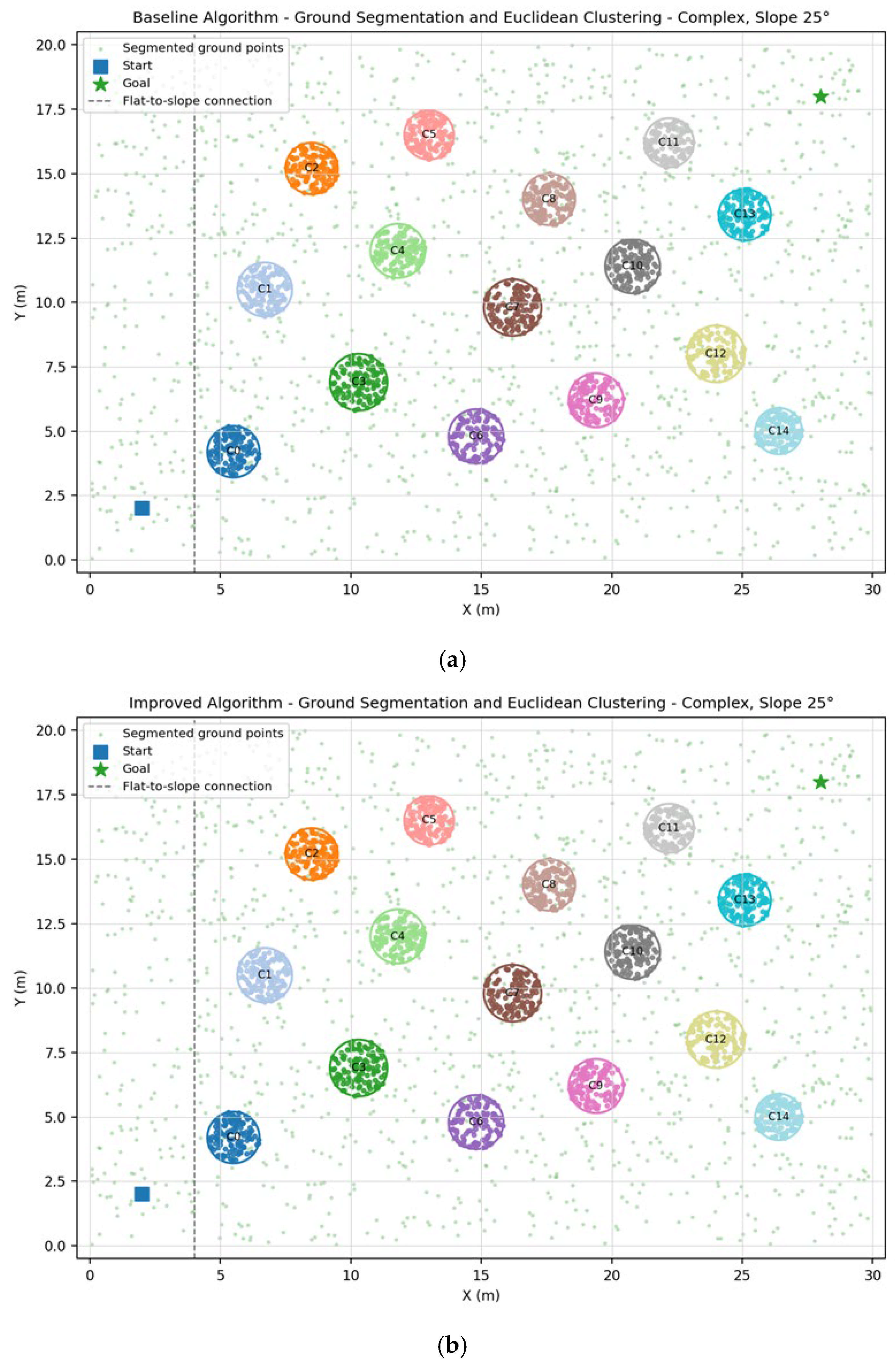
Figure 10 shows that IMU-adaptive ground segmentation improved the stability of non-ground point extraction on sloped terrain. The proposed algorithm maintained high obstacle recall under different slope and environment conditions, whereas the recall of the baseline algorithm decreased more rapidly as slope and environment complexity increased.

3.1.3. Ablation Study

To analyze the influence of key modules on system performance, a module-level ablation study was conducted on the basis of the complete proposed algorithm. The overall multi-sensor fusion autonomous navigation framework was retained, and three key modules were removed separately:
  • IMU-adaptive ground segmentation was removed, and only the fixed-threshold Ray Ground Filter was retained.
  • The slope-aware path cost was removed, and only the distance-based path cost was retained.
  • Slope-adaptive velocity regulation was removed, and conventional Pure Pursuit tracking control was retained.
Except for the removed module, the sensor configuration, map, start and goal positions, obstacle settings, and evaluation metrics remained consistent with those of the complete proposed algorithm. This design minimized the influence of non-target factors on the interpretation of ablation results. The ablation study was also conducted under three environments and five slope conditions, and the arrival rate, tracking RMSE, localization RMSE, dynamic safety clearance, obstacle recall, and clustering precision were statistically analyzed.
As shown in Table 7, after removing IMU-adaptive ground segmentation, the tracking RMSE, localization RMSE, and dynamic safety clearance remained nearly unchanged, whereas obstacle recall decreased from 98.65% to 87.51% and clustering precision decreased from 98.58% to 80.33%. This result should be interpreted as a perception-chain ablation rather than as evidence that IMU-adaptive ground segmentation has no influence on closed-loop navigation. In the current simulation implementation, the segmentation result was not fully fed back into obstacle map updating, path planning, and control-loop execution. Therefore, a complete closed-loop ablation experiment should be conducted in future work to further evaluate the indirect influence of this module on path safety and control performance.
After removing the slope-aware path cost, the arrival rate decreased from 100.0% to 86.7%, the collision rate increased from 0.0% to 13.3%, and the tracking RMSE increased from 0.218 m to 0.280 m. This is because a purely distance-based cost tends to select geometrically shorter paths without actively avoiding high-slope risk areas or regions close to obstacles. Such paths may be short but unsafe in complex hilly terrain.
After removing slope-adaptive velocity regulation, the localization RMSE increased from 0.280 m to 0.358 m, and the minimum dynamic safety clearance decreased from 2.308 m to 1.630 m. This indicates that slope–curvature-coupled velocity regulation plays an important role in improving closed-loop stability during uphill motion and turning. When the chassis maintains conventional speed output on high-slope sections, attitude disturbance and yaw oscillation may be amplified.
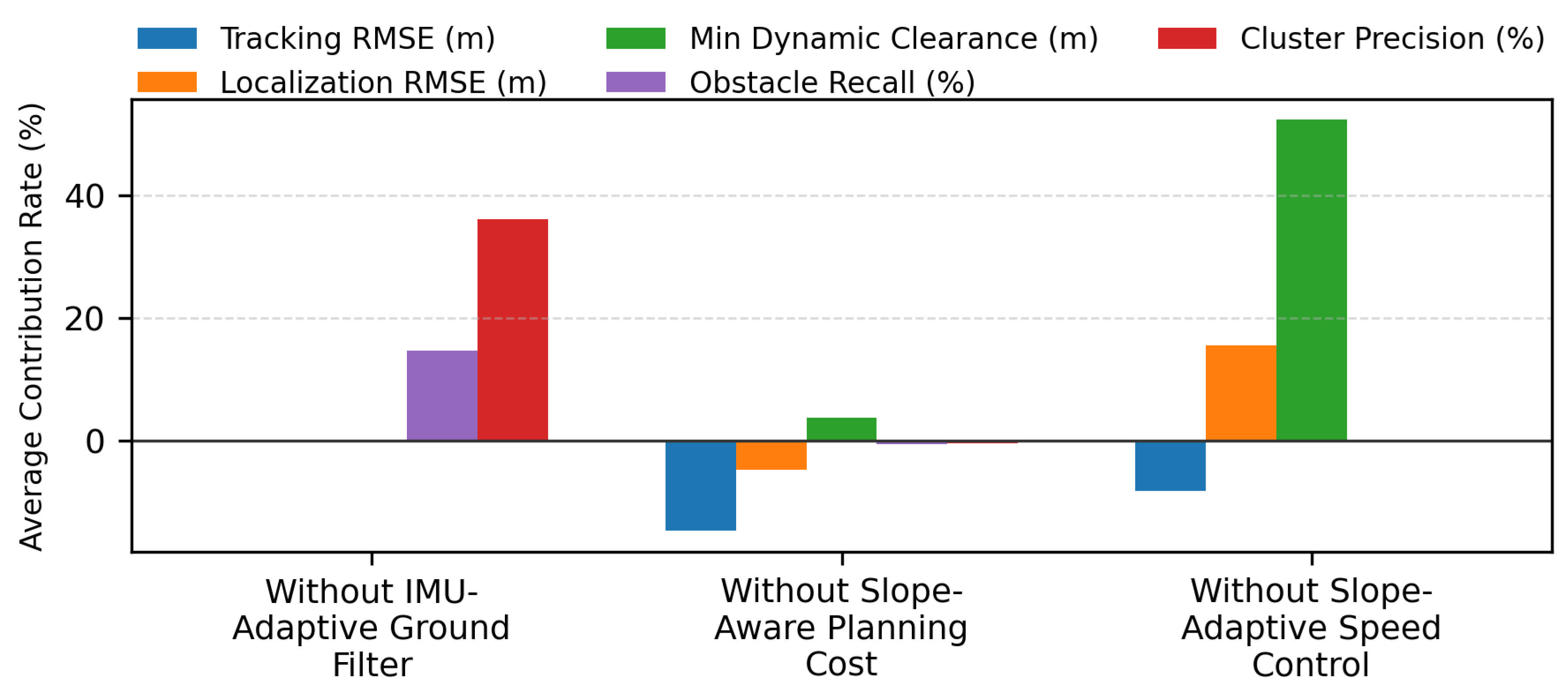
To quantify the relative contribution of each key module to the complete proposed algorithm, a module contribution rate was defined based on the ablation results. Let M f u l l be the value of a given metric for the complete proposed algorithm, and let M a b l be the value of the same metric after removing a module. For error-type metrics, such as tracking RMSE and localization RMSE, where smaller values indicate better performance, the contribution rate is defined as
C m = M a b l M f u l l M a b l × 100 % ,
For positive metrics, such as dynamic safety clearance, obstacle recall, and clustering precision, where larger values indicate better performance, the contribution rate is defined as
C m + = M f u l l M a b l M a b l × 100 % ,
where C m denotes the relative reduction rate of error-type metrics achieved by the complete proposed algorithm compared with the ablation version, and C m + denotes the relative improvement rate of positive metrics. A positive contribution rate indicates that the removed module contributed to the complete system performance, whereas a value close to zero indicates a weak influence on the corresponding metric.
Table 8 and Figure 11 show the contribution rates of different modules. IMU-adaptive ground segmentation contributed most clearly to obstacle recall and clustering precision. The slope-aware path cost mainly improved path reachability, collision risk reduction, and tracking stability. Slope-adaptive velocity regulation contributed most strongly to dynamic safety clearance and localization stability.

3.1.4. Summary of Python Simulation Results

The Python deterministic trend results in Table 5 and Table 6 and Figure 7, Figure 8, Figure 9 and Figure 10 show that the proposed algorithm generally achieved lower tracking RMSE and localization RMSE, while dynamic safety clearance improved in several deterministic scenarios. The statistical interpretation of dynamic safety clearance should be combined with the repeated-trial significance tests in Section 3.3.7.
The Python simulation adopted idealized globally constant slope conditions and was mainly used to compare the influence of slope and obstacle complexity on algorithm performance. Under this setting, the baseline algorithm was more likely to suffer from increased tracking error, accumulated localization error, and insufficient safety clearance in high-slope or obstacle-dense environments because it did not explicitly consider slope risk, odometry drift, near-field dynamic obstacle safety zones, or slope-adaptive velocity regulation. Therefore, the Python simulation results are more suitable for evaluating the statistical performance differences between the two algorithms under systematically controlled conditions.
The ablation study further showed that different modules affected system performance through different mechanisms. IMU-adaptive ground segmentation mainly improved obstacle recall and clustering precision; slope-aware path cost mainly improved path reachability, collision risk reduction, and tracking stability; and slope-adaptive velocity regulation mainly improved localization stability and dynamic safety clearance. These results indicate that the performance advantage of the proposed method was achieved through the coordinated effects of perception, localization, planning, and control, rather than through a single isolated module.

3.2. ROS/Gazebo Representative Scenario Validation

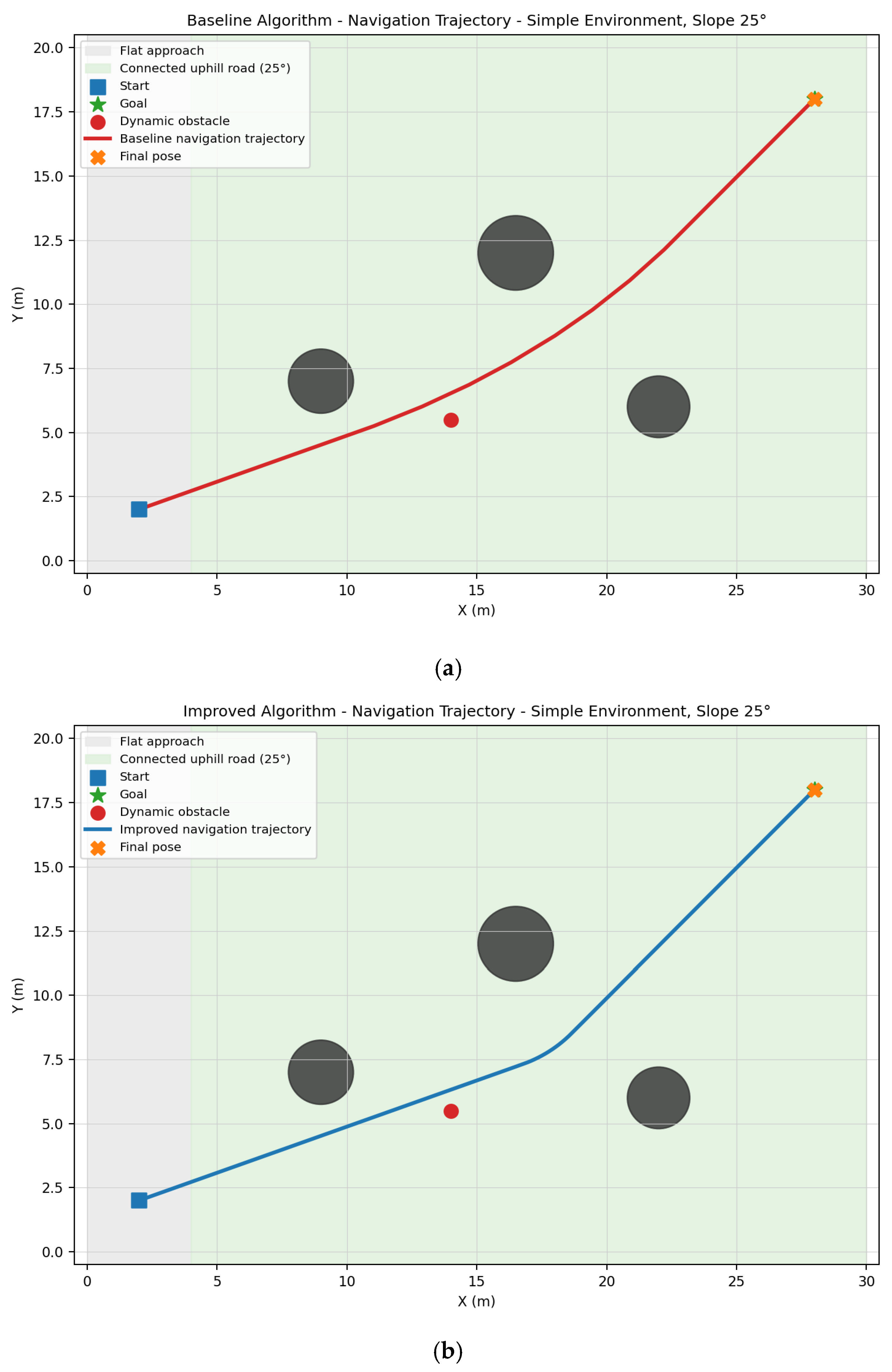
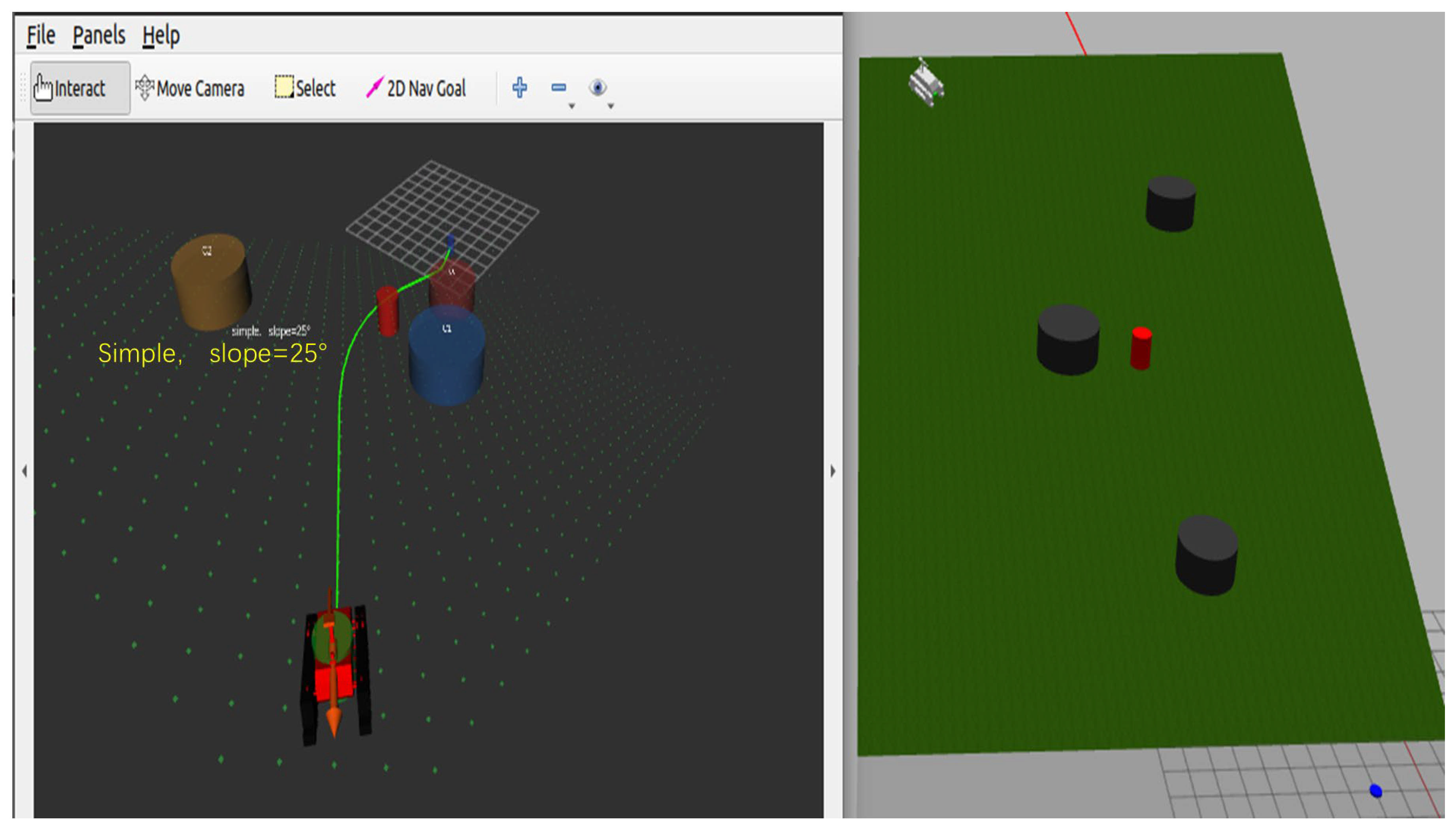
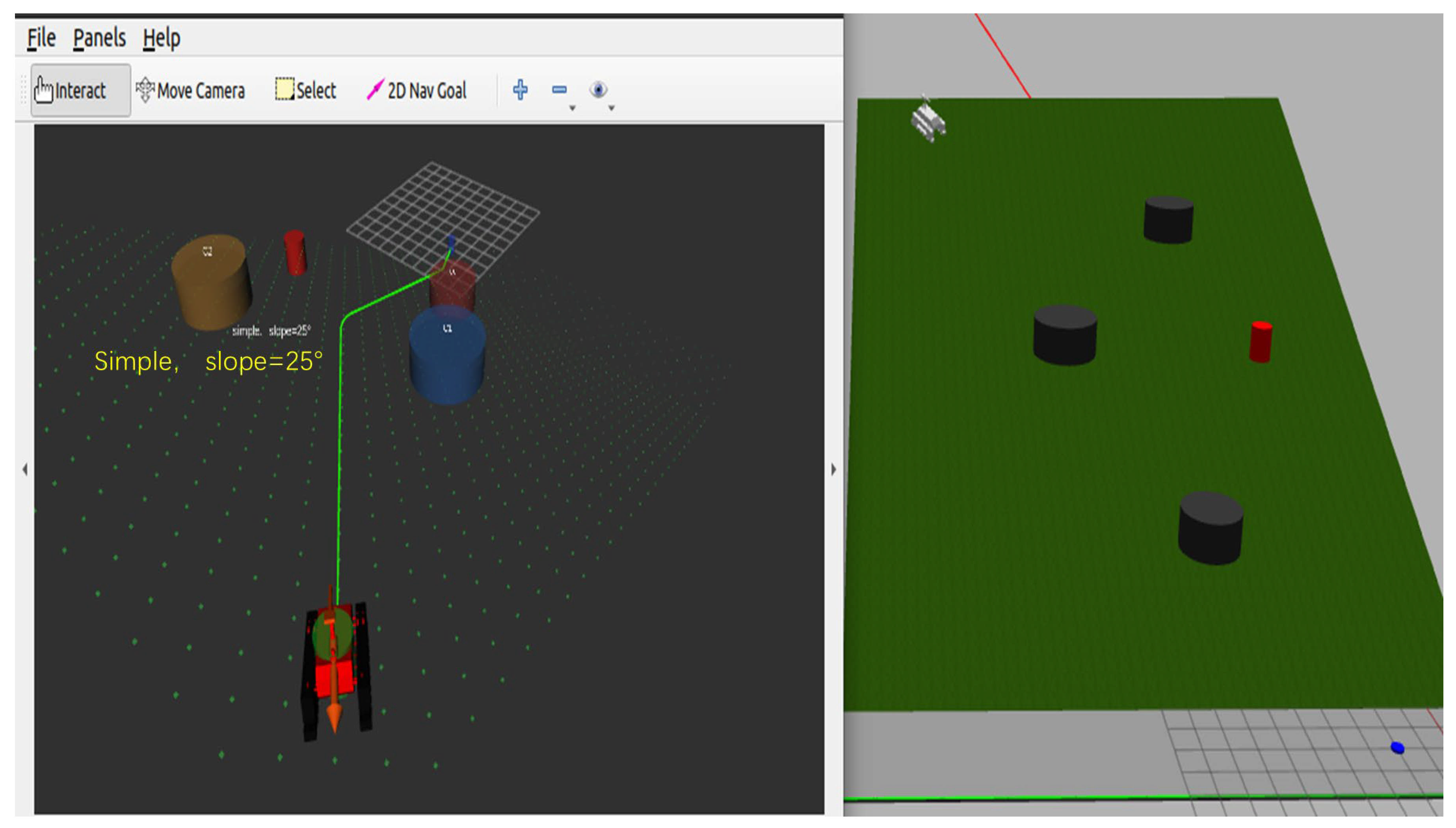
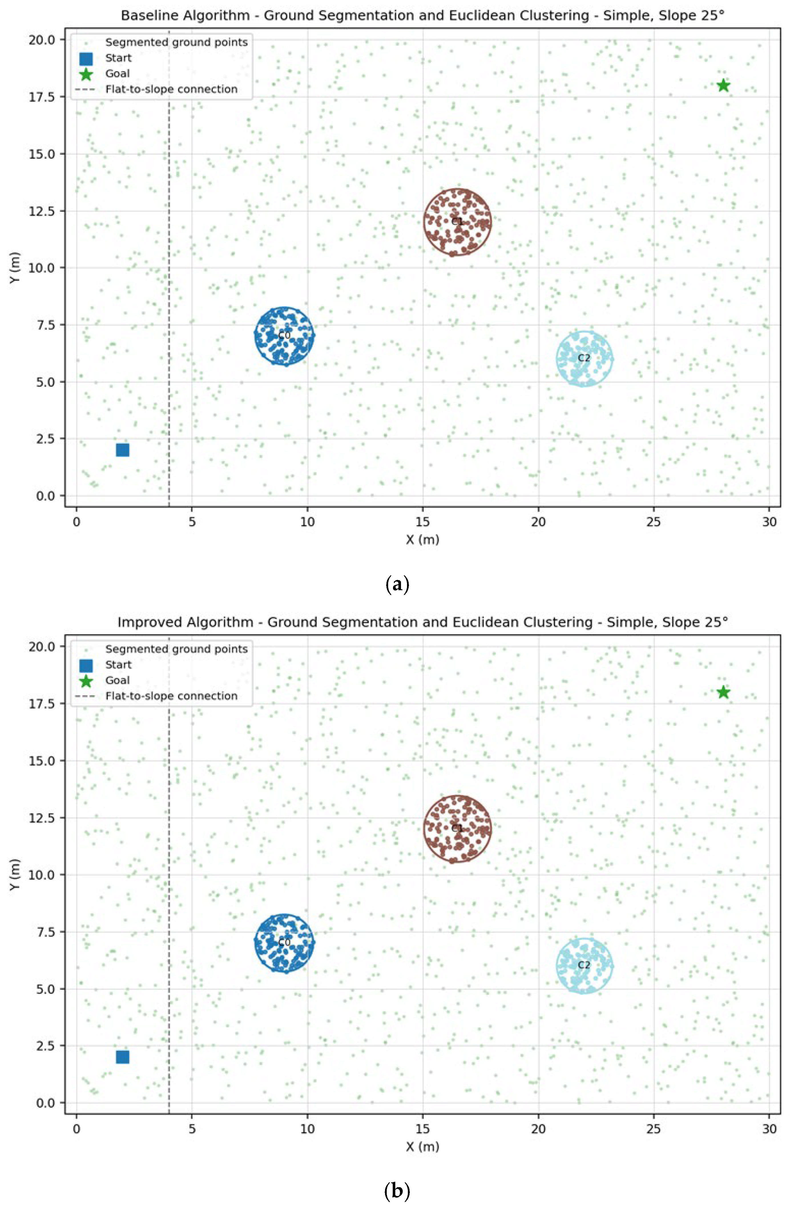
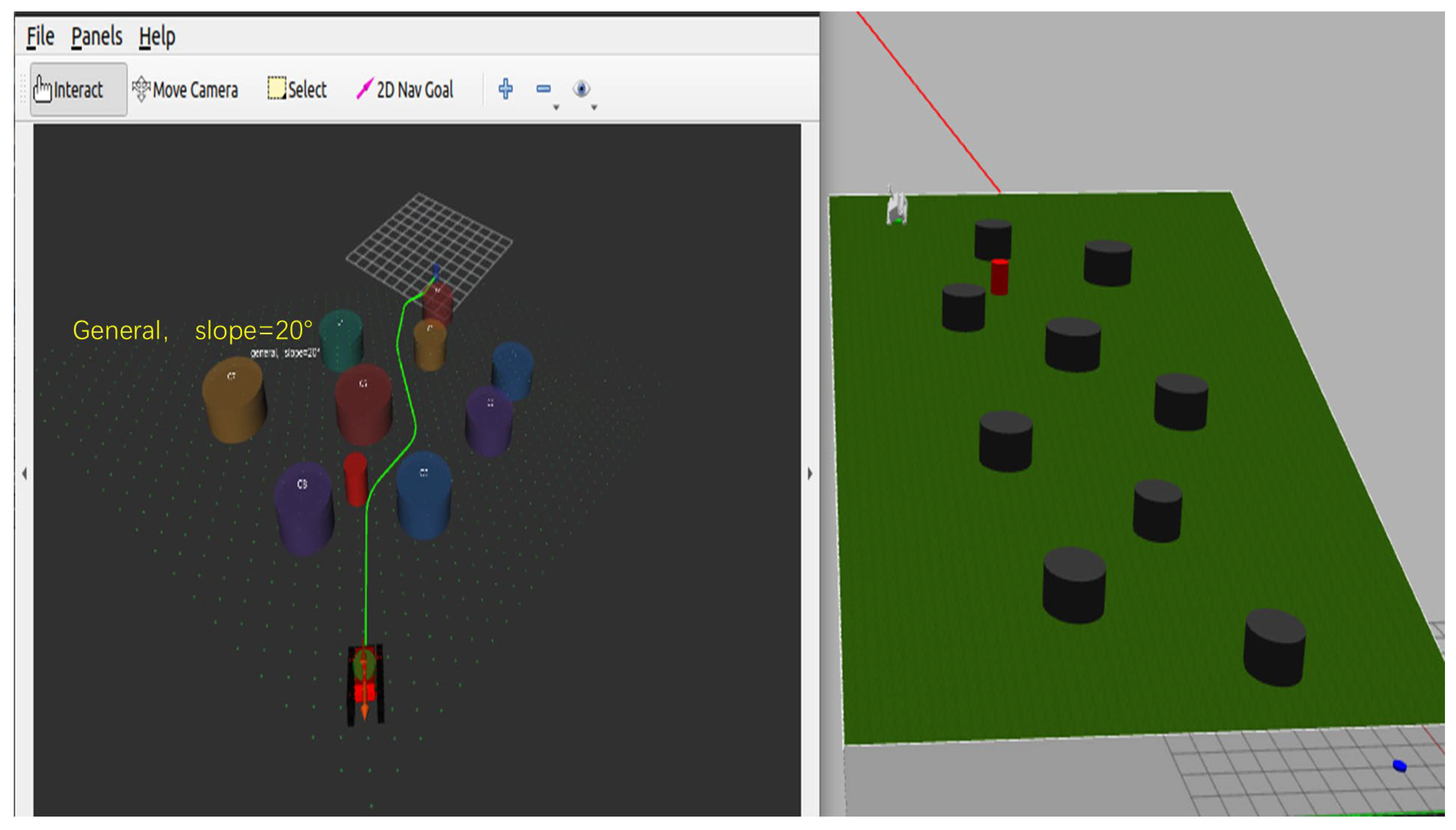
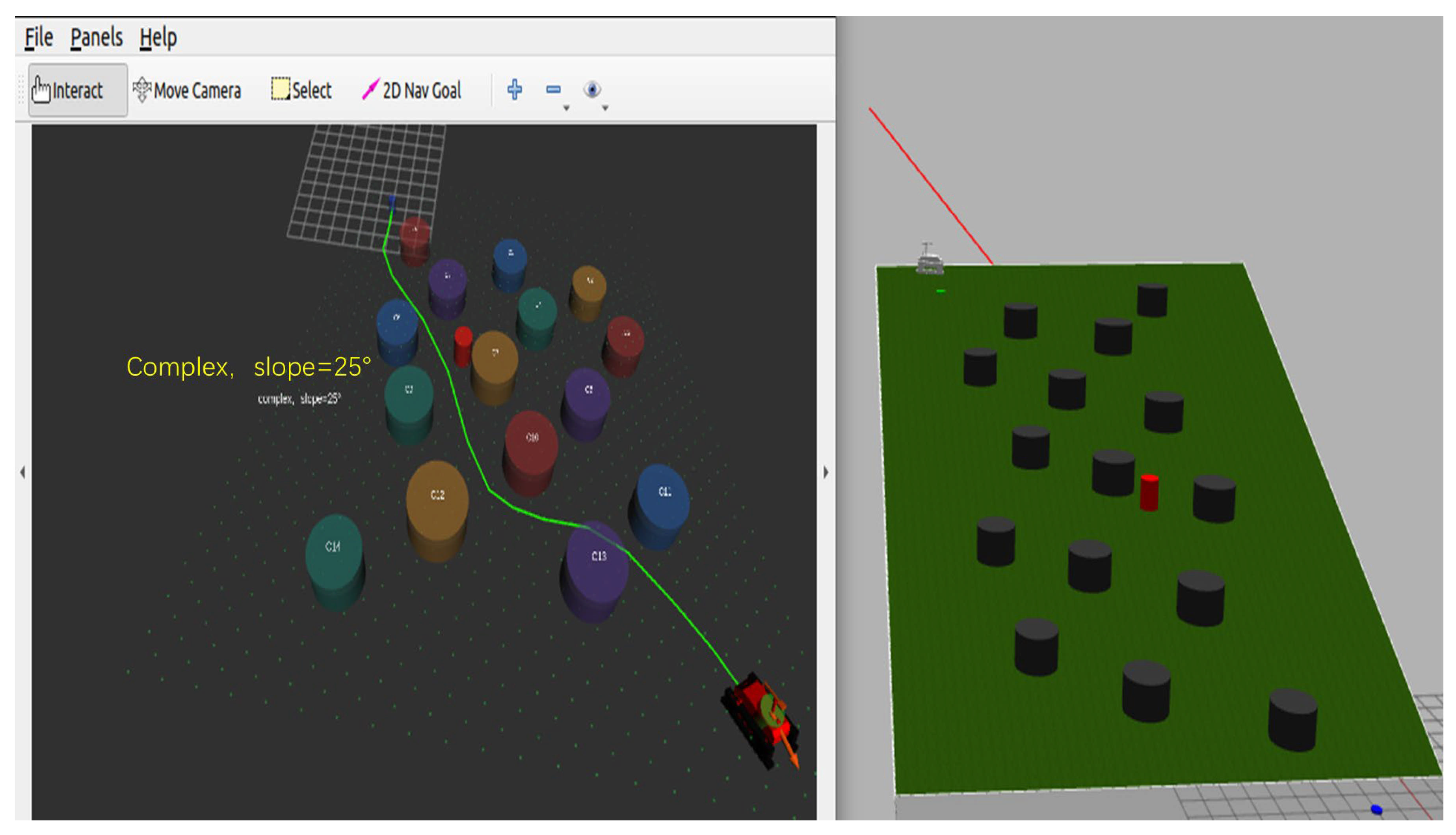
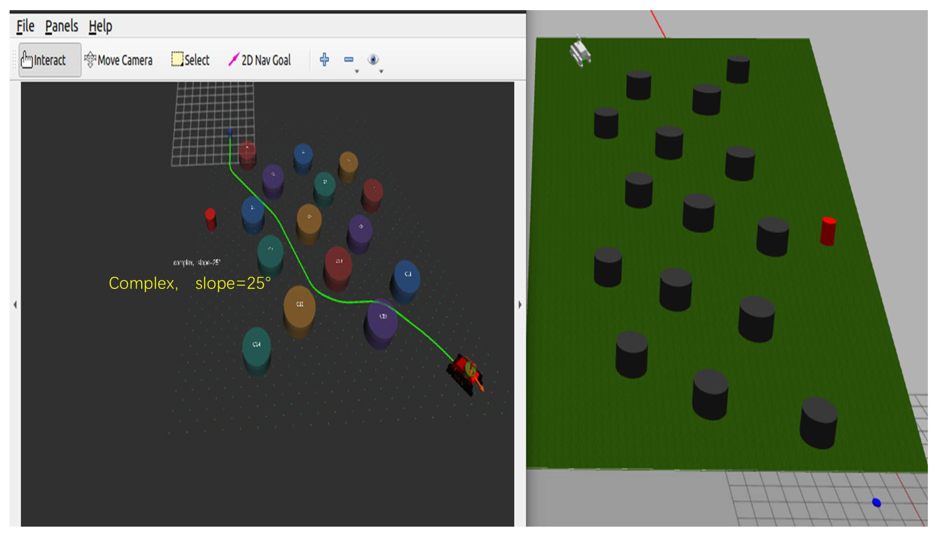
Because this study included three environment types, five slope conditions, and two algorithms, presenting all trajectory plots, point cloud clustering results, and intermediate process figures in the main text would make the manuscript overly lengthy and reduce the clarity of the main findings. Therefore, three representative scenarios were selected for ROS/Gazebo engineering visualization validation: the simple environment at 25°, the general environment at 20°, and the complex environment at 25°. These scenarios represent basic stability under high-slope conditions, comprehensive performance under moderate obstacle constraints, and obstacle avoidance under strong constraints, respectively.
The ROS/Gazebo simulation was conducted in Ubuntu 20.04 with ROS Noetic. A tracked agricultural chassis model was used in Gazebo, and the terrain consisted of a flat section, a transition section, and a constant-slope section. The chassis started from the initial point, stabilized on the flat section, entered the sloped section through the transition section, and finally reached the target point. RViz was used to visualize the chassis pose, trajectory, map, and point cloud processing results. In the Gazebo scenes, the red cylindrical object represents the dynamic obstacle, while the other cylindrical objects represent static obstacles. All result figures were recorded after the chassis reached the target point and stopped navigation and mapping.
It should be noted that the ROS/Gazebo simulation was mainly used to evaluate the operational consistency and visualization performance of the navigation process in an engineering simulation environment. It was not intended to replace the full statistical results obtained from the Python simulations.

3.2.1. Overall Metrics of Representative ROS/Gazebo Scenarios

Table 9 presents the ROS/Gazebo simulation metrics for the three representative scenarios. All six runs reached the target point without collision, indicating that both the baseline and proposed algorithms could complete the navigation task in the selected engineering simulation scenarios. However, compared with the baseline algorithm, the proposed algorithm showed better overall performance in trajectory smoothness, steering stability, and obstacle safety clearance.
In the simple environment at 25°, the proposed algorithm reduced the heading-rate standard deviation from 0.4092 to 0.0730, reduced the trajectory smoothness index from 17.2089 to 1.6489, and increased P5 obstacle clearance from 0.8282 m to 1.0166 m. In the general environment at 20°, the heading-rate standard deviation decreased from 1.8233 to 0.0971, the trajectory smoothness index decreased from 74.2537 to 0.9509, and P5 obstacle clearance increased from 0.4539 m to 0.5713 m. In the complex environment at 25°, the proposed algorithm reduced the heading-rate standard deviation from 2.7714 to 0.8666, reduced the trajectory smoothness index from 112.5679 to 31.8226, and increased P5 obstacle clearance from 0.4489 m to 0.5685 m.
Table 10 summarizes the scenario-wise improvement rates of the proposed algorithm relative to the baseline algorithm based on the raw metrics reported in Table 9. For heading-rate standard deviation and trajectory smoothness index, lower values indicate smoother and more stable motion; therefore, the reduction rate was calculated. For robust obstacle clearance P5, a higher value indicates a larger safety margin around obstacles; therefore, the improvement rate was calculated.
The columns “Baseline mean” and “Proposed mean” represent the arithmetic mean values of the corresponding raw metrics across the three representative scenarios in Table 9. The column “Mean scenario-wise improvement” represents the arithmetic mean of the three scenario-wise improvement rates. Therefore, this value is not calculated directly from the aggregated baseline and proposed means. This definition separates raw metric averaging from relative improvement averaging and avoids confusion caused by different statistical denominators.
As shown in Table 10, the proposed algorithm reduced the heading-rate standard deviation by an average of 81.86% and the trajectory smoothness index by 86.96% across the three representative ROS/Gazebo scenarios. The robust P5 obstacle clearance increased by an average of 25.08%. These results indicate that the proposed method produced smoother trajectory execution and maintained larger obstacle safety margins in the selected ROS/Gazebo engineering validation scenarios.
Figure 12, Figure 13, Figure 14 and Figure 15 provide visual comparisons of the ROS/Gazebo trajectory-execution metrics. Figure 12, Figure 14 and Figure 15 correspond to the quantitative metrics summarized in Table 9 and Table 10, including heading-rate standard deviation, trajectory smoothness index, and robust P5 obstacle clearance. Figure 13 provides an additional post-processed trajectory-geometry visualization based on resampled curvature variance, which is used only as supplementary visual evidence and is not included in the scenario-wise improvement table in order to keep Table 9 and Table 10 statistically consistent.
Overall, the trends shown in Figure 12, Figure 14 and Figure 15 are consistent with Table 9 and Table 10, indicating that the proposed algorithm achieved smoother steering behavior, lower trajectory oscillation, and larger obstacle safety margins in the representative ROS/Gazebo engineering simulation scenarios.
Figure 12, Figure 13, Figure 14 and Figure 15 compare the baseline and proposed algorithms in terms of heading-rate standard deviation, resampled curvature variance, trajectory smoothness index, and robust P5 obstacle clearance. Among these metrics, heading-rate standard deviation, trajectory smoothness index, and robust P5 obstacle clearance are the main quantitative ROS/Gazebo metrics reported in Table 9 and Table 10. The resampled curvature variance shown in Figure 13 is retained as supplementary post-processed trajectory-geometry evidence, but it is not included in Table 10 because its raw values are not listed in Table 9.
For heading-rate standard deviation, resampled curvature variance, and trajectory smoothness index, lower values indicate better stability and smoother motion. For P5 obstacle clearance, a higher value indicates a larger robust safety margin around obstacles. The trends shown in Figure 12, Figure 14 and Figure 15 are consistent with the quantitative results in Table 9 and Table 10, indicating that the proposed algorithm completed navigation with smoother trajectories and greater safety margins in the engineering simulation environment.

3.2.2. Simple Environment at 25°

The simple environment at 25° was used to evaluate the basic stability of the system under high-slope conditions. Because this environment had sparse obstacles and sufficient traversable space, the main challenge was not obstacle density but the stability of localization and path tracking under increased slope. In this scenario, both the baseline and proposed algorithms reached the target point. However, as shown in Table 9, the proposed algorithm achieved a lower heading-rate standard deviation and trajectory smoothness index while maintaining a larger P5 obstacle clearance. This indicates that, under high-slope conditions with weak obstacle constraints, the main benefit of the proposed algorithm was improved attitude adaptation and smoother trajectory execution.
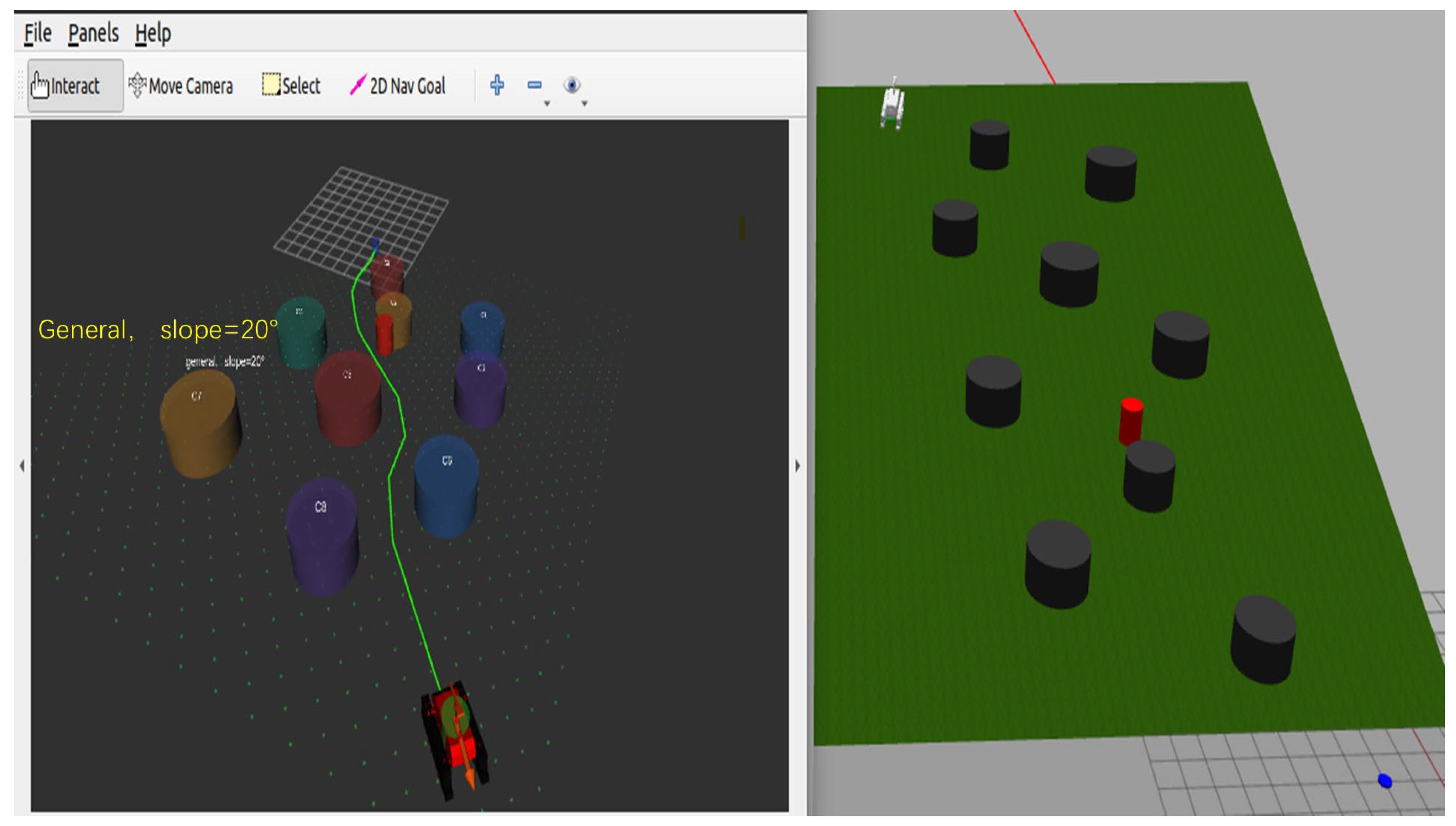
The simulation results are shown in Figure 16, Figure 17, Figure 18 and Figure 19. Figure 16 and Figure 17 present the Gazebo/RViz visualization results of the baseline and proposed algorithms, respectively. Figure 18 compares the executed trajectories of the two algorithms, where Figure 18a shows the baseline algorithm and Figure 18b shows the proposed algorithm. Figure 19 compares the point cloud ground segmentation and Euclidean clustering results, where Figure 19a shows the baseline algorithm and Figure 19b shows the proposed algorithm.

3.2.3. General Environment at 20°

The general environment at 20° was used to represent a scenario with a medium-to-high slope and moderate obstacle density. Compared with the simple environment, this scenario involved more frequent path curvature changes and stronger obstacle constraints.
As shown in Table 9, in this scenario, the proposed algorithm reduced the heading-rate standard deviation from 1.8233 to 0.0971, reduced the trajectory smoothness index from 74.2537 to 0.9509, and increased P5 obstacle clearance from 0.4539 m to 0.5713 m. These results indicate that the proposed algorithm not only maintained better passability on sloped terrain but also achieved a more favorable balance between trajectory smoothness and obstacle safety margin.
The simulation results are shown in Figure 20, Figure 21, Figure 22 and Figure 23. Figure 20 and Figure 21 present the Gazebo/RViz visualization results of the baseline and proposed algorithms, respectively. Figure 22 compares the executed trajectories of the two algorithms, where Figure 22a shows the baseline algorithm and Figure 22b shows the proposed algorithm. Figure 23 compares the point cloud ground segmentation and Euclidean clustering results, where Figure 23a shows the baseline algorithm and Figure 23b shows the proposed algorithm.

3.2.4. Complex Environment at 25°

The complex environment at 25° was the most constrained representative scenario, with both the maximum slope and the highest obstacle density. This scenario was used to evaluate whether the algorithm could maintain stable steering and safety clearance in a narrow-channel navigation condition. The simulation results are shown in Figure 24, Figure 25, Figure 26 and Figure 27.
The results show that although the baseline algorithm could reach the target point in this representative ROS/Gazebo scenario, it exhibited larger heading fluctuations and less smooth motion. In contrast, the proposed algorithm reduced the heading-rate standard deviation to 0.8666, reduced the trajectory smoothness index to 31.8226, and increased P5 obstacle clearance to 0.5685 m.
It is important to note that, in the full Python statistical results, the average arrival rate of the baseline algorithm in the complex environment was only 20.0%, whereas the baseline algorithm reached the target point in the complex ROS/Gazebo representative scenario. This difference mainly results from the different validation objectives and scenario constructions. The Python results were obtained from 15 environment–slope combinations under globally constant slope conditions and were used for statistical evaluation. In contrast, the ROS/Gazebo result was obtained from a selected representative engineering visualization scenario that included a flat section, a transition section, and a constant-slope section. Therefore, the successful arrival of the baseline algorithm in the ROS/Gazebo scenario does not contradict the Python statistical results. Rather, it indicates that the baseline algorithm could still complete the task in the selected representative engineering scenario, while its stability and safety margins were inferior to those of the proposed algorithm.
The simulation results are shown in Figure 24, Figure 25, Figure 26 and Figure 27. Figure 24 and Figure 25 present the Gazebo/RViz visualization results of the baseline and proposed algorithms, respectively. Figure 26 compares the executed trajectories of the two algorithms, where Figure 26a shows the baseline algorithm and Figure 26b shows the proposed algorithm. Figure 27 compares the point cloud ground segmentation and Euclidean clustering results, where Figure 27a shows the baseline algorithm and Figure 27b shows the proposed algorithm.

3.2.5. Summary of ROS/Gazebo Simulation Results

The ROS/Gazebo engineering visualization results in Table 9 and Table 10 and Figure 12, Figure 13, Figure 14, Figure 15, Figure 16, Figure 17, Figure 18, Figure 19, Figure 20, Figure 21, Figure 22, Figure 23, Figure 24, Figure 25, Figure 26 and Figure 27 show that both the baseline and proposed algorithms completed the basic navigation tasks in the selected representative scenarios. However, compared with the baseline algorithm, the proposed algorithm achieved better trajectory smoothness, steering stability, and obstacle safety clearance in all three scenarios. The improvements in heading-rate standard deviation, trajectory smoothness index, and P5 obstacle clearance were particularly evident in the general and complex environments. These three metrics were selected as the main ROS/Gazebo quantitative indicators because their raw values were directly reported in Table 9 and their scenario-wise improvement rates were summarized in Table 10. The resampled curvature variance was retained only as a supplementary trajectory-geometry visualization in Figure 13.
These results indicate that the proposed method not only improved key performance metrics in the Python statistical simulations but also showed better operational consistency in the ROS/Gazebo engineering simulation environment. Nevertheless, the ROS/Gazebo results should be interpreted as representative engineering visualization validation rather than a substitute for the full statistical evaluation or real-field experiments. Real hilly farmland field tests are still required to further verify the practical applicability of the proposed method.

3.3. Supplementary Statistical and Robustness Validation

To further verify the robustness and statistical reliability of the proposed method, additional analyses were conducted, including multi-seed repeated trials, IMU slope-prior perturbation tests, path cost weight sensitivity analysis, stronger-baseline comparison, mixed perturbation stress testing, no-LakiBeam1L ablation, and statistical significance tests. These analyses provide supplementary evidence for evaluating the stability, repeatability, and system-level effectiveness of the proposed method under simulation conditions.

3.3.1. Multi-Seed Repeated Trials and Confidence Intervals

A total of 10 repeated runs were performed for each environment–slope–algorithm combination, resulting in 150 records for the baseline algorithm and 150 records for the proposed algorithm. Table 11 shows the overall mean ± standard deviation across the repeated-trial dataset. The proposed method substantially improved the arrival rate, collision rate, tracking RMSE, localization RMSE, obstacle recall, and clustering precision. The mean dynamic safety clearance was comparable between the two methods, but the proposed method achieved that clearance with far fewer failures and lower variability. Therefore, the repeated-trial results support the conclusion that the proposed method is more repeatable and statistically more reliable than the baseline under the present simulation setup.
Based on the unrounded repeated-trial dataset, the proposed method reduced the collision rate by 92.86%, reduced tracking RMSE by 61.46%, and reduced localization RMSE by 60.62%. Obstacle recall and clustering precision also improved by 26.32% and 35.14%, respectively. Figure 28 plots the 95% confidence intervals for three representative continuous metrics and shows that the proposed method achieved both lower means and tighter intervals for tracking and localization errors.

3.3.2. IMU Slope-Prior Robustness Under Vibration, Drift, and Dynamic Motion

Because the IMU prior is used by ground segmentation, slope-aware planning, and velocity regulation, an additional perturbation test was carried out by replaying the proposed trajectories under four conditions: nominal noise, vibration, drift, and combined dynamic motion. Table 12 and Figure 29 report the overall mean ± standard deviation of slope estimation RMSE, slope estimation MAE, the 95th-percentile absolute slope error, obstacle recall, and clustering precision.
The dynamic-motion condition produced the largest perturbation, but the overall slope RMSE was still only 0.82°, and the 95th-percentile absolute error remained 1.48°. These errors are much smaller than the 7° terrain undulation allowance used in the adaptive ground segmentation threshold, which explains why obstacle recall remained above 98.75% in all tested conditions. Therefore, the additional IMU analysis supports the use of the IMU-derived slope prior within the current simulation perturbation envelope, while also making it explicit that this validation is still simulation-based rather than hardware-bench-based.
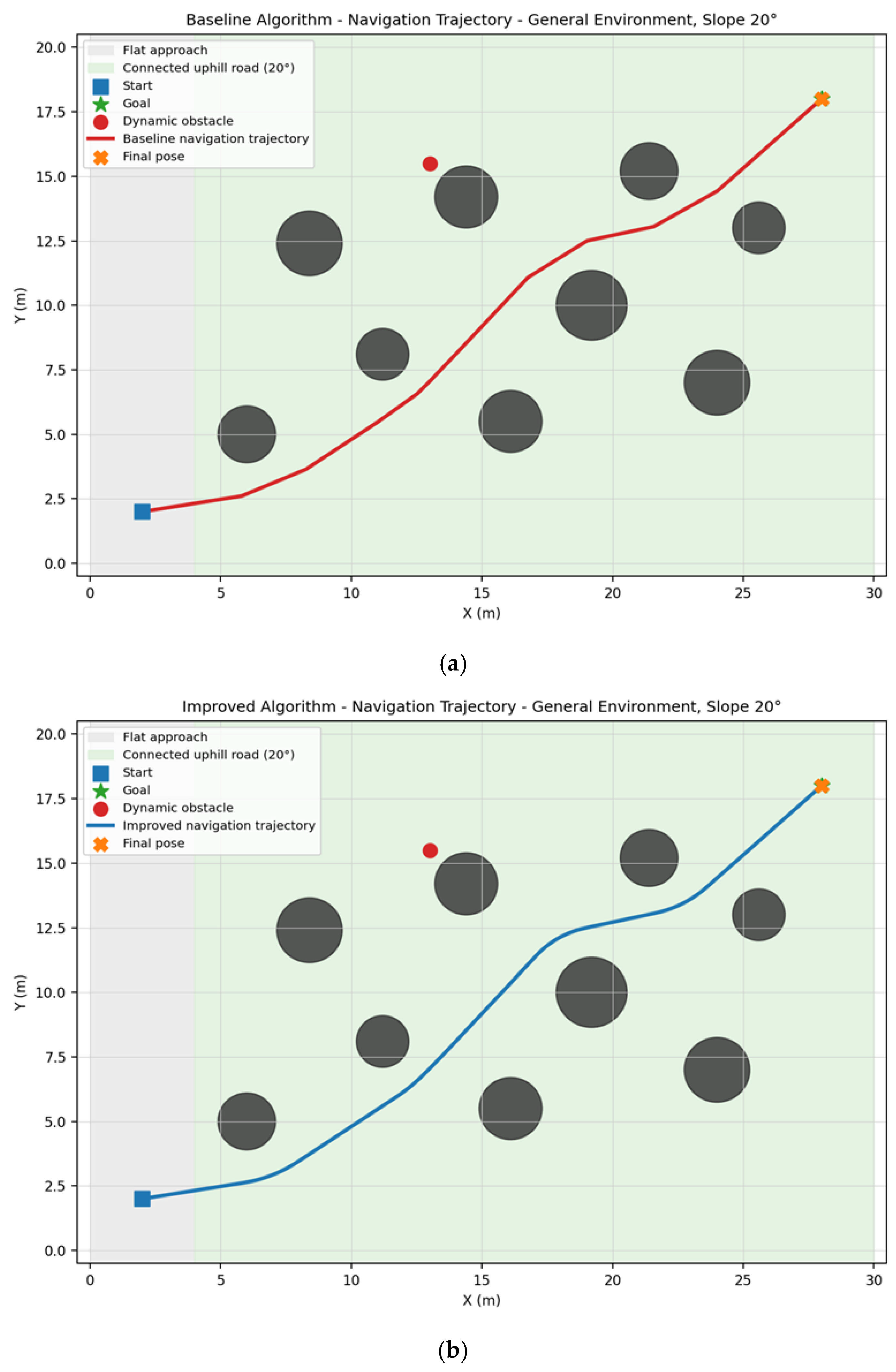
3.3.3. Path Cost Weight Sensitivity Analysis

A one-at-a-time sensitivity analysis was conducted for the path-planning parameters k s , k c , k o and σ . Each parameter was swept over five candidate values while the remaining parameters were fixed at their nominal settings. Table 13 summarizes the stable intervals observed in the 15 environment–slope cases, and Figure 30 visualizes the variation in arrival rate and dynamic safety clearance.
Three main conclusions can be drawn from the sensitivity study. First, the selected values k s = 1.8 and σ = 1.6 were located within stable intervals, whereas k o = 0.65 was the only tested value that maintained the full arrival rate under the current sensitivity setting. Second, the obstacle potential weight k o was the most sensitive planning parameter, because reducing it weakened safety margin maintenance, whereas increasing it over-penalized near-obstacle corridors and reduced arrival rate. Third, the cross-slope weight k c produced almost no topology change in the current synthetic terrain over 0.2–1.4, indicating that the present slope field was not overly sensitive to moderate variations in this weight. This result clarifies both the robustness of some parameters and the sensitivity of the obstacle potential term.

3.3.4. Comparison Against Stronger Baselines

To reduce the risk of overclaiming improvement against a weak baseline, two stronger baselines were added: NDT-ICP + A* + conventional Pure Pursuit, and NDT-ICP + A* + DWA. Table 14 and Figure 31 report their repeated-trial statistics together with the original baseline and the proposed method.
The stronger baseline comparison clarifies that the proposed method is not uniformly best on every isolated metric. The NDT-ICP + A* + conventional Pure Pursuit baseline achieved a slightly smaller tracking RMSE than the proposed method, but at the cost of a much lower arrival rate, a much higher collision rate, and a much smaller dynamic safety margin. By contrast, the proposed method outperformed NDT-ICP + A* + DWA in tracking RMSE, localization RMSE, and dynamic safety clearance simultaneously. Therefore, the advantage of the proposed method should be interpreted as a better system-level trade-off among perception quality, stability, safety margin, and task completion, rather than as a monotonic improvement on every single local metric.

3.3.5. Mixed Perturbation Stress Test

To further test robustness beyond the original constant-case simulations, a mixed perturbation stress test was added. The perturbations included random obstacle-position offsets, additional sensor noise perturbation, initial-position and initial-heading perturbation, dynamic obstacle speed perturbation, and a non-constant slope model with gradual variation and local terrain undulation. Each environment-slope-algorithm combination was repeated five times, resulting in 75 records for the baseline and 75 records for the proposed method. The results are summarized in Table 15 and Figure 32.
Under the mixed perturbation setting, the proposed method maintained an arrival rate of 81.3%, whereas the baseline reached only 29.3%. The collision rate decreased from 70.7% to 18.7%, tracking RMSE decreased from 0.617 m to 0.278 m, localization RMSE decreased from 0.693 m to 0.290 m, and obstacle recall increased from 84.58% to 98.13%. These results show that the proposed method retained its main advantages when obstacle layout, sensing noise, initial pose, dynamic obstacle speed, and slope morphology were perturbed simultaneously.

3.3.6. No-LakiBeam1L Ablation and Near-Field Response Latency

To evaluate whether the additional single-line LiDAR is justified, an isolated no-LakiBeam1L ablation was added. In this ablation, the proposed perception, localization, slope-aware planning, and slope-adaptive control modules were retained, but the LakiBeam1L velocity-dependent near-field trigger and local re-planning signal were disabled. Table 16 and Figure 33 summarize the ablation results.
To further support this design choice, Table 17 reports the algorithmic latency benchmark between the LakiBeam1L trigger and the C16 point-cloud clustering pipeline.
The no-LakiBeam1L ablation reduced arrival rate from 90.7% to 76.0%, increased collision rate from 9.3% to 24.0%, and reduced dynamic safety clearance from 2.322 m to 1.982 m. It produced a slightly lower tracking RMSE, but this was obtained with less conservative behavior and a smaller safety margin. The latency benchmark also shows why the C16 point cloud pipeline should not be the only emergency-trigger channel: in the Python implementation, the direct LakiBeam1L trigger required 0.0176 ms on average, whereas the C16 segmentation-and-clustering pipeline required 12.25 ms. This benchmark measures algorithmic processing time rather than hardware scan period, but it supports the design choice that the single-line LiDAR is a low-latency auxiliary safety channel rather than a replacement for 3D LiDAR perception.

3.3.7. Statistical Significance Tests

Welch’s t-tests and Mann–Whitney U tests were conducted for continuous metrics in the 10-seed repeated-trial dataset. Fisher’s exact test was used for binary arrival and collision outcomes. The tests were used to support statistical interpretation, but not to claim field-level performance because all samples were still generated in simulation.
The corresponding statistical test results are summarized in Table 18.
The significance tests confirmed statistically significant differences for arrival rate, collision rate, tracking RMSE, localization RMSE, obstacle recall, and clustering precision. The dynamic safety clearance difference was not statistically significant in the repeated-trial aggregate, which is why the revised manuscript interprets this metric more cautiously and avoids claiming universal superiority on every isolated metric.

4. Discussion

Before discussing the effectiveness of the proposed method, it is useful to clarify the relation between perception metrics and navigation metrics in this study. The IMU-adaptive ground segmentation mainly affects obstacle recall and clustering precision. These perception gains do not automatically translate into lower tracking RMSE in every case, because the latter is more directly influenced by localization, path geometry, and speed regulation. By contrast, the slope-aware path cost mainly affects path feasibility and collision exposure, whereas the slope-adaptive velocity controller mainly affects dynamic safety clearance and closed-loop motion stability.

4.1. Effectiveness Analysis of the Proposed Method

First, the reduction in tracking RMSE under complex environments and medium-to-high slope conditions is consistent with the velocity regulation mechanism based on slope angle and heading error, as defined in Equations (26)–(29). As the slope angle and steering demand increase, the controller actively reduces the linear velocity, thereby alleviating sideslip and trajectory oscillation during sharp turning on sloped terrain. Second, the reduction in localization RMSE is consistent with the NDT matching-cost optimization defined in Equations (6) and (7). This process enables pose estimation to be constrained by the point cloud map rather than relying solely on odometry, thereby reducing accumulated pose errors under track-slip conditions. These mechanisms have been described in the Materials and Methods Section: NDT scan-to-map matching is used in the mapping and localization layer, slope-adaptive Pure Pursuit is used in the control layer, and slope risk, cross-slope risk, and obstacle-distance constraints are incorporated into the edge cost in the global planning layer.
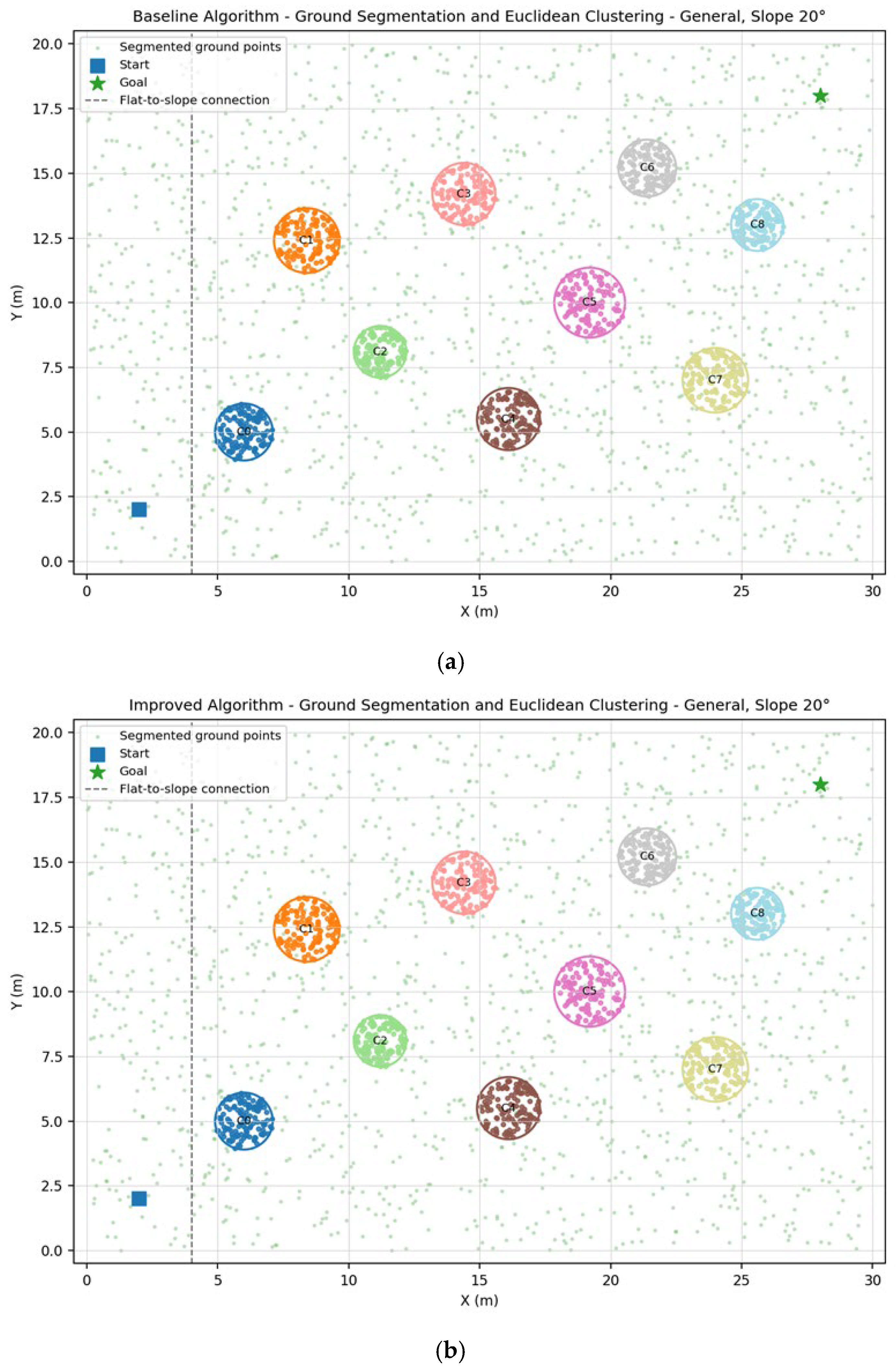
The improvements in dynamic safety clearance and obstacle recall can also be explained by the ground segmentation, planning, and safety-triggering models. The improvement in obstacle recall corresponds to the IMU-adaptive ground-threshold mechanism described in Equations (9)–(11). The increase in dynamic safety clearance is jointly related to the obstacle potential terms in Equations (15) and (20), the local A* re-planning and dynamic obstacle inflation mechanisms in Equations (22) and (23), and the velocity-dependent safety zone defined in Equations (32) and (33). Therefore, the larger safety margin obtained by the proposed algorithm results from the combined effects of perception, planning, and control. Together with the Python simulation results, the ROS/Gazebo validation further indicates that the advantages of the proposed algorithm are reflected not only in localization and perception-related metrics, but also in smoother trajectory execution and larger obstacle safety margins.
The results indicate that the main advantages of the proposed algorithm include improved arrival rate, reduced collision rate, lower localization and tracking errors, and more stable perception quality. Dynamic clearance improved in several deterministic and perturbation settings, but the repeated-trial aggregate did not show a statistically significant difference; therefore, this metric is interpreted as scenario-dependent rather than universally improved.

4.2. Differences Between Python Simulation and ROS/Gazebo Validation

This study used both Python batch simulation and ROS/Gazebo representative scenario validation. These two simulation platforms differ in validation purpose and scenario construction. Therefore, the results should be interpreted by distinguishing between statistical performance evaluation and engineering visualization validation.
The Python simulation included all combinations of three environment types and five slope conditions, and the slope was idealized as globally constant across the whole simulation area. This setting is suitable for analyzing the influence of slope and obstacle complexity on algorithm performance under controlled conditions. Because the slope remained constant throughout the simulation area, the baseline algorithm was continuously affected by odometry drift, fixed-speed tracking, and insufficient dynamic safety clearance in high-slope and complex environments. Consequently, the average arrival rate of the baseline algorithm was relatively low in the complex environment.
In contrast, the ROS/Gazebo simulation adopted an engineering terrain structure consisting of a flat section, a transition section, and a constant-slope section. Its main purpose was to verify the consistency of the chassis model, sensor coordinate relationships, path execution process, and RViz/Gazebo visualization results. The chassis had a short stabilization process on the flat section before entering the slope, and only three representative scenarios were selected for visualization. Therefore, the fact that the baseline algorithm reached the target point in the ROS/Gazebo simulations does not contradict the Python statistical results. Rather, it indicates that the baseline algorithm could still complete the navigation task in the selected representative scenarios, while its steering stability and safety margin remained weaker than those of the proposed algorithm, as reflected by the heading-rate standard deviation, trajectory smoothness index, and P5 obstacle clearance.
Thus, the interpretation of the two types of simulation results should remain clearly bounded. Python simulation was used to evaluate statistical performance differences under multiple slope and environment combinations, whereas ROS/Gazebo simulation was used to evaluate operational consistency and visualization performance in an engineering simulation platform. The two forms of validation are complementary, but the ROS/Gazebo representative scenarios cannot replace the full Python statistical evaluation, and neither simulation result should be directly regarded as evidence of real-field performance in hilly farmland.

4.3. Limitations

Although the proposed method showed promising performance under the designed simulation conditions, several limitations remain.
  • This study mainly conducted Python batch simulation and ROS/Gazebo representative engineering visualization validation. Real-vehicle experiments in hilly farmland have not yet been carried out.
  • The interaction between the track and soil was simplified. A complete model considering track slip, soil sinkage, and adhesion variation has not yet been established.
  • Sensor noise, time-synchronization error, and mechanical vibration were also simplified in the current simulation. In real agricultural environments, these factors may affect point cloud registration, ground segmentation, obstacle detection, and control stability.
  • The dynamic obstacle model was mainly used to verify the safety-triggering and local-avoidance logic. More complex scenarios involving multiple pedestrians, multiple vehicles, irregularly moving targets, and occlusion were not considered.
These limitations indicate that future work should include real hilly farmland experiments, more realistic track–soil interaction modeling, and hardware-level verification of the IMU slope prior under vibration and long-duration drift. Although the revised manuscript now includes repeated trials, perturbation-based IMU validation, planning-weight sensitivity analysis, and stronger baseline comparison, these additions still remain simulation-based. They strengthen methodological rigor, but they do not remove the need for bench tests and real-field experiments on actual hilly farmland.

4.4. Comparison with Existing Studies

Compared with recent studies on agricultural robot navigation, the present study differs in both the research object and the coupling characteristics of the problem. Most existing studies focus on orchards, greenhouses, or general unstructured agricultural environments and often aim to improve the performance of a single module. However, fewer studies have systematically addressed the coupled effects of track-slip-induced localization drift, slope-induced ground point cloud misclassification, slope-aware mapping and localization, cross-slope risk, and near-field safety triggering for dynamic obstacles. For tracked agricultural chassis operating in hilly farmland, the main challenge is not only the limited performance of an individual module, but also the interaction among slope variation, track slip, sloped-ground misclassification, cross-slope risk, and dynamic obstacle disturbance.
The main feature of this study is the construction of a closed-loop navigation framework for tracked agricultural chassis in hilly farmland by integrating slope priors, point cloud constraints, risk-aware planning, and velocity-adaptive control. Compared with single-module optimization methods, the proposed method places greater emphasis on system-level coordination under continuously varying slopes and significant cross-slope risks. The simulation results show that the proposed method can achieve a more balanced trade-off among safety, stability, and passability in high-slope and highly constrained scenarios.

5. Conclusions

This study proposed a multi-sensor fusion autonomous navigation method for a tracked agricultural chassis operating in hilly farmland, with the aim of improving safe passability and localization stability under continuously varying slope conditions. The proposed method integrates a nine-axis IMU, a Leishen C16 mechanical LiDAR, and a LakiBeam1L single-line LiDAR. IMU-derived slope attitude priors, Leishen C16 point cloud geometric constraints, slope–cross-slope joint path costs, and velocity-dependent near-field safety control were incorporated into a unified closed-loop navigation framework. The effectiveness of the method under simulated conditions was evaluated through Python batch simulations and ROS/Gazebo representative scenario validation. The main conclusions are as follows:
  • Slope information should not be used only as an attitude measurement result; instead, it can serve as a terrain prior throughout perception, planning, and control.
  • Under the present simulation setup, IMU-prior-aided NDT localization and slope-adaptive velocity control reduced repeated-trial tracking and localization errors, while IMU-adaptive ground segmentation mainly improved obstacle recall and clustering precision.
  • For tracked agricultural chassis operating in hilly farmland, navigation should prioritize stability and safety margins rather than simply pursuing the shortest path or minimum travel time.
  • Python batch simulation and ROS/Gazebo representative scenario validation serve different purposes. Therefore, the simulation results should not be directly interpreted as equivalent to real-vehicle field-test results.
The simulation results under three environments and five slope conditions indicate that the proposed algorithm achieved a better overall trade-off than the baseline algorithm in repeated-trial arrival rate, collision rate, tracking RMSE, localization RMSE, obstacle recall, and clustering precision. However, the analyses also show that some single metrics, such as mean dynamic clearance in the repeated-trial aggregate or tracking RMSE under one stronger baseline, are not uniformly dominated. Accordingly, the main claim of this study is a system-level improvement in stability, perception reliability, and task completion under simulated hilly conditions, rather than universal superiority on every isolated metric.
Although the proposed method showed promising performance in simulation, several limitations remain. The current work has mainly completed Python-based batch metric evaluation and ROS/Gazebo engineering visualization validation, while real-vehicle experiments in hilly farmland have not yet been conducted. Future work will focus on the following aspects:
  • Conducting real-vehicle experiments in hilly farmland and establishing field datasets to verify the simulation-based conclusions of this study.
  • Introducing a more complete track–soil interaction model and incorporating slip, sinkage, adhesion, and surface conditions into a unified dynamic analysis framework.
  • Further improving sensor error modeling and time-synchronization mechanisms to enhance the adaptability of the system to complex real-world operating conditions.
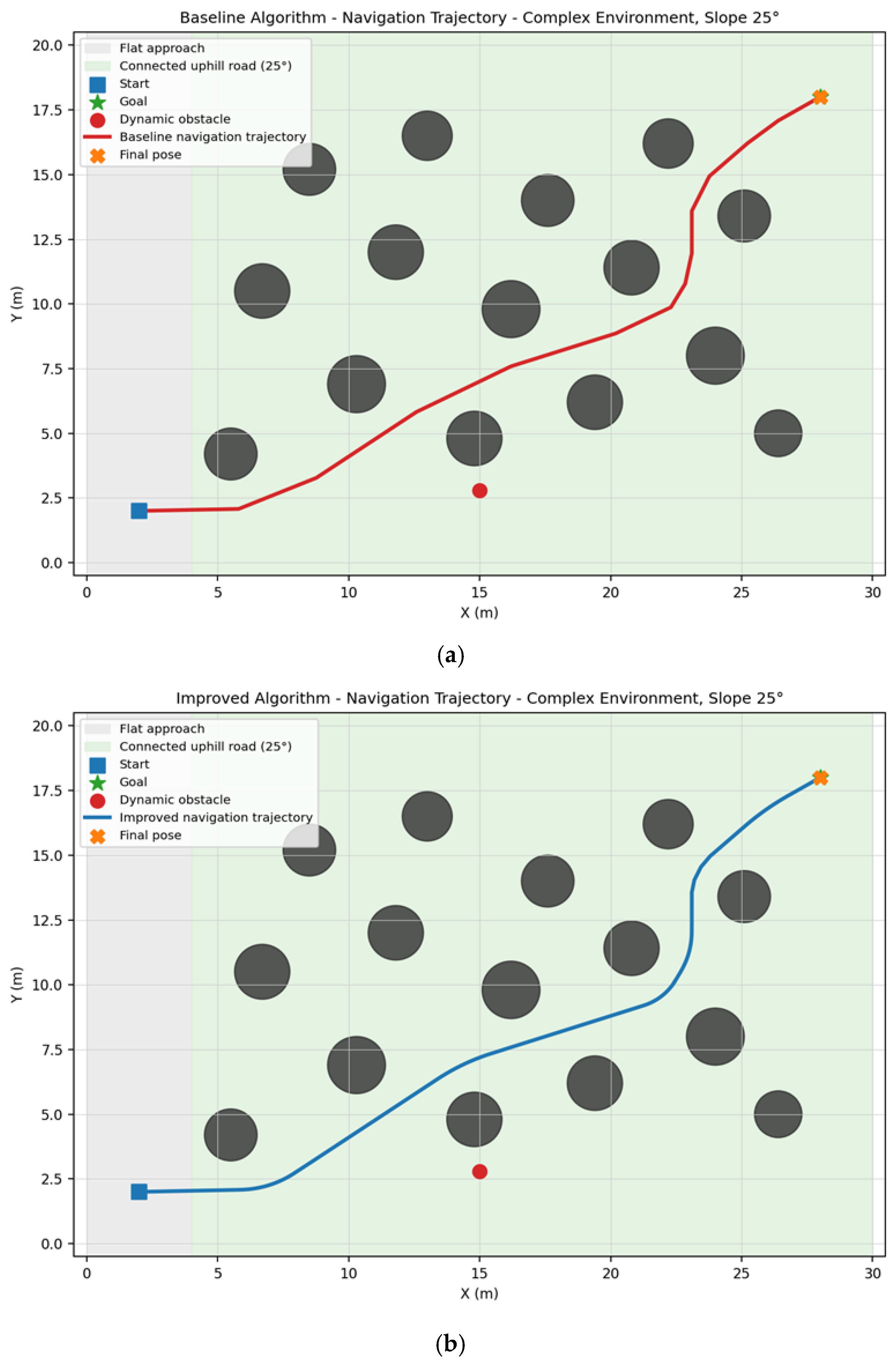
  • Extending the complexity of dynamic obstacle scenarios and investigating risk prediction and cooperative obstacle avoidance under conditions involving multiple pedestrians, multiple vehicles, and irregularly moving targets.
  • Performing long-duration batch simulations for all environment–slope combinations in ROS/Gazebo to establish a more complete engineering statistical database, thereby supporting subsequent system iteration and real-vehicle deployment.

Author Contributions

Conceptualization, W.Z., B.L. and H.Z.; methodology, W.Z. and B.L.; validation, W.Z., B.L., Y.P. and X.S.; formal analysis, W.Z. and B.L.; resources, W.Z. and H.Z.; data curation, W.Z. and B.L.; writing—original draft preparation, W.Z. and B.L.; writing—review and editing, W.Z., B.L., X.S., Y.P., T.S., X.X. and H.Z.; visualization, W.Z., B.L. and Y.P.; supervision, B.L. and H.Z.; project administration, B.L. and H.Z.; funding acquisition, W.Z. and H.Z. All authors have read and agreed to the published version of the manuscript.

Funding

This research was funded by the China Central Fund for Guiding Development of Local Science and Technology under Grant No. 202407AB110010, the Yunnan Science and Technology Major Project under Grant No. 202302AE090020, the Yunnan Science and Technology Major Project under Grant No. 202303AP140014, and the Yunnan Provincial Key Research and Development Plan under Grant No. 202603AS090008.

Institutional Review Board Statement

Not applicable.

Informed Consent Statement

Not applicable.

Data Availability Statement

The original contributions presented in this study are included in the article. Further inquiries can be directed to the corresponding author.

Acknowledgments

The authors thank all members of the research team for their assistance during platform modeling, simulation construction, and data analysis. During the preparation of this manuscript, the authors used ChatGPT (GPT-5.1) to assist with improving clarity, grammar, and phrasing of selected text passages. The tool was not used to generate scientific content, experimental results, data, figures, or interpretations. All outputs were carefully reviewed and edited by the authors, who take full responsibility for the content of this publication.

Conflicts of Interest

The authors declare no conflicts of interest.

References

  1. Ding, R.; Qi, X.; Meng, X.; Chen, X.; Zhang, L.; Mei, Y.; Li, A.; Ye, Q. A Review on the Chassis Configurations and Key Technologies of Agricultural Robots. Agriculture 2025, 15, 2379. [Google Scholar] [CrossRef] [Scilit]
  2. Wu, H.; Wang, X.; Chen, X.; Zhang, Y.; Zhang, Y. Review on Key Technologies for Autonomous Navigation in Field Agricultural Machinery. Agriculture 2025, 15, 1297. [Google Scholar] [CrossRef] [Scilit]
  3. Wang, R.-F.; Xu, R.; Chee, P.W.; Wang, H.; Li, C. A Review of Visual Navigation for Agricultural Robots in Open Fields and Controlled Environments. Comput. Electron. Agric. 2026, 248, 111754. [Google Scholar] [CrossRef] [Scilit]
  4. Yao, X.; Zhang, B.; Wang, X.; Su, Y.; Cao, G.; Bian, Y. Adaptive Navigation for Robots in Unstructured Agricultural Environments Using Stable Feature Localization and Multi-Sensor Obstacle Detection. Comput. Electron. Agric. 2025, 234, 110302. [Google Scholar] [CrossRef] [Scilit]
  5. Fujinaga, T. Autonomous Navigation Method for Agricultural Robots in High-Bed Cultivation Environments. Comput. Electron. Agric. 2025, 231, 110001. [Google Scholar] [CrossRef] [Scilit]
  6. Jiang, S.; Qi, P.; Han, L.; Liu, L.; Li, Y.; Huang, Z.; He, X. Navigation System for Orchard Spraying Robot Based on 3D LiDAR SLAM with NDT-ICP Point Cloud Registration. Comput. Electron. Agric. 2024, 220, 108870. [Google Scholar] [CrossRef] [Scilit]
  7. Hong, Y.; Ma, R.; Li, C.; Shao, C.; Huang, J.; Zeng, Y.; Chen, Y. Three-Dimensional Localization and Mapping of Multiagricultural Scenes via Hierarchically-Coupled LiDAR-Inertial Odometry. Comput. Electron. Agric. 2024, 227, 109487. [Google Scholar] [CrossRef] [Scilit]
  8. Huang, Z.; Yang, N.; Cao, R.; Li, Z.; He, Y.; Feng, X. Autonomous Navigation System in Various Greenhouse Scenarios Based on Improved FAST-LIO2. Comput. Electron. Agric. 2025, 234, 110279. [Google Scholar] [CrossRef] [Scilit]
  9. Nakaguchi, V.M.; Abeyrathna, R.M.R.D.; Liu, Z.; Noguchi, R.; Ahamed, T. Development of a Machine Stereo Vision-Based Autonomous Navigation System for Orchard Speed Sprayers. Comput. Electron. Agric. 2024, 227, 109669. [Google Scholar] [CrossRef] [Scilit]
  10. Li, Q.; Zhu, H. Performance Evaluation of 2D LiDAR SLAM Algorithms in Simulated Orchard Environments. Comput. Electron. Agric. 2024, 221, 108994. [Google Scholar] [CrossRef] [Scilit]
  11. Rakun, J.; Duchoň, F.; Lepej, P. Spatial LiDAR Odometry and Mapping for Complex Agricultural Environments: Spatial FieldLOAM. Biosyst. Eng. 2024, 248, 58–72. [Google Scholar] [CrossRef] [Scilit]
  12. Teng, H.; Wang, Y.; Chatziparaschis, D.; Karydis, K. Adaptive LiDAR Odometry and Mapping for Autonomous Agricultural Mobile Robots in Unmanned Farms. Comput. Electron. Agric. 2025, 232, 110023. [Google Scholar] [CrossRef] [Scilit]
  13. Wang, W.; Qin, J.; Huang, D.; Zhang, F.; Liu, Z.; Wang, Z.; Yang, F. Integrated Navigation Method for Orchard-Dosing Robot Based on LiDAR/IMU/GNSS. Agronomy 2024, 14, 2541. [Google Scholar] [CrossRef] [Scilit]
  14. Wang, Y.; Fu, C.; Huang, R.; Tong, K.; He, Y.; Xu, L. Path Planning for Mobile Robots in Greenhouse Orchards Based on Improved A* and Fuzzy DWA Algorithms. Comput. Electron. Agric. 2024, 227, 109598. [Google Scholar] [CrossRef] [Scilit]
  15. Cho, I.; Chung, W. Learning Self-Supervised Traversability with Navigation Experiences of Mobile Robots: A Risk-Aware Self-Training Approach. IEEE Robot. Autom. Lett. 2024, 9, 4122–4129. [Google Scholar] [CrossRef] [Scilit]
  16. Cao, G.; Zhang, B.; Li, Y.; Wang, Z.; Diao, Z.; Zhu, Q.; Liang, Z. Environmental Mapping and Path Planning for Robots in Orchard Based on Traversability Analysis, Improved LeGO-LOAM and RRT* Algorithms. Comput. Electron. Agric. 2025, 230, 109889. [Google Scholar] [CrossRef] [Scilit]
  17. Jiang, Q.; Shen, Y.; Liu, H.; Khan, Z.; Sun, H.; Huang, Y. A Hybrid Path Planning Algorithm for Orchard Robots Based on an Improved D* Lite Algorithm. Agriculture 2025, 15, 1698. [Google Scholar] [CrossRef] [Scilit]
  18. Rottok, L.; Zhou, J.; Wang, Y.; Zizhen, J.; Gemechu, T.T.; Syed, T.N.; Aurangzaib, M.; Chepkemoi, M. Development of a LiDAR-Based Framework for Obstacle Identification and Mapping in Orchard Environments. Biosyst. Eng. 2025, 257, 104245. [Google Scholar] [CrossRef] [Scilit]
  19. Li, H.; Huang, K.; Sun, Y.; Lei, X.; Yuan, Q.; Zhang, J.; Lv, X. An Autonomous Navigation Method for Orchard Mobile Robots Based on Octree 3D Point Cloud Optimization. Front. Plant Sci. 2025, 15, 1510683. [Google Scholar] [CrossRef] [Scilit] [PubMed]
  20. Hu, C.; Ru, Y.; Li, X.; Fang, S.; Zhou, H.; Yan, X.; Xie, R. Path Tracking Control for Brake-Steering Tracked Vehicles Based on an Improved Pure Pursuit Algorithm. Biosyst. Eng. 2024, 242, 1–15. [Google Scholar] [CrossRef] [Scilit]
  21. Cheng, J.; Zhang, B.; Zhang, C.; Zhang, Y.; Shen, G. A Model-Free Adaptive Predictive Path-Tracking Controller with PID Terms for Tractors. Biosyst. Eng. 2024, 242, 38–49. [Google Scholar] [CrossRef] [Scilit]
  22. Song, Y.; Xue, J.; Zhang, T.; Sun, X.; Sun, H.; Gao, W.; Chen, Q. Path Tracking Control of Crawler Tractor Based on Adaptive Adjustment of Lookahead Distance Using Sparrow Search Algorithm. Comput. Electron. Agric. 2025, 234, 110219. [Google Scholar] [CrossRef] [Scilit]
  23. Chen, D.; Wang, Q.; Lin, Y.; Ma, Z.; Sun, L.; Yu, G. Path Tracking Control of Paddy Field Weeder Integrated with Satellite and Visual Methods. Comput. Electron. Agric. 2025, 234, 110257. [Google Scholar] [CrossRef] [Scilit]
  24. Zhang, S.; Wei, X.; Liu, C.; Ge, J.; Cui, X.; Wang, F.; Chen, W. Adaptive Path Tracking and Control System for Unmanned Crawler Harvesters in Paddy Fields. Comput. Electron. Agric. 2025, 230, 109878. [Google Scholar] [CrossRef] [Scilit]
  25. Liu, H.; Han, Z.; Yin, J.; Bao, J.; Mu, J.; Tan, H.; Liu, X. Path Tracking Control Method for Tracked Agricultural Vehicles Based on Slip-Aware Look-Ahead Point Offset. Front. Plant Sci. 2026, 16, 1754679. [Google Scholar] [CrossRef] [Scilit]
  26. Wei, J.; Zhao, Z.; Lu, E.; Liu, S.; Hu, X.; Zhou, Q.; Xu, C. Adaptive Backstepping Tracking Control for Differential Drive Vehicles under Longitudinal Slipping Conditions. Biosyst. Eng. 2026, 261, 104339. [Google Scholar] [CrossRef] [Scilit]
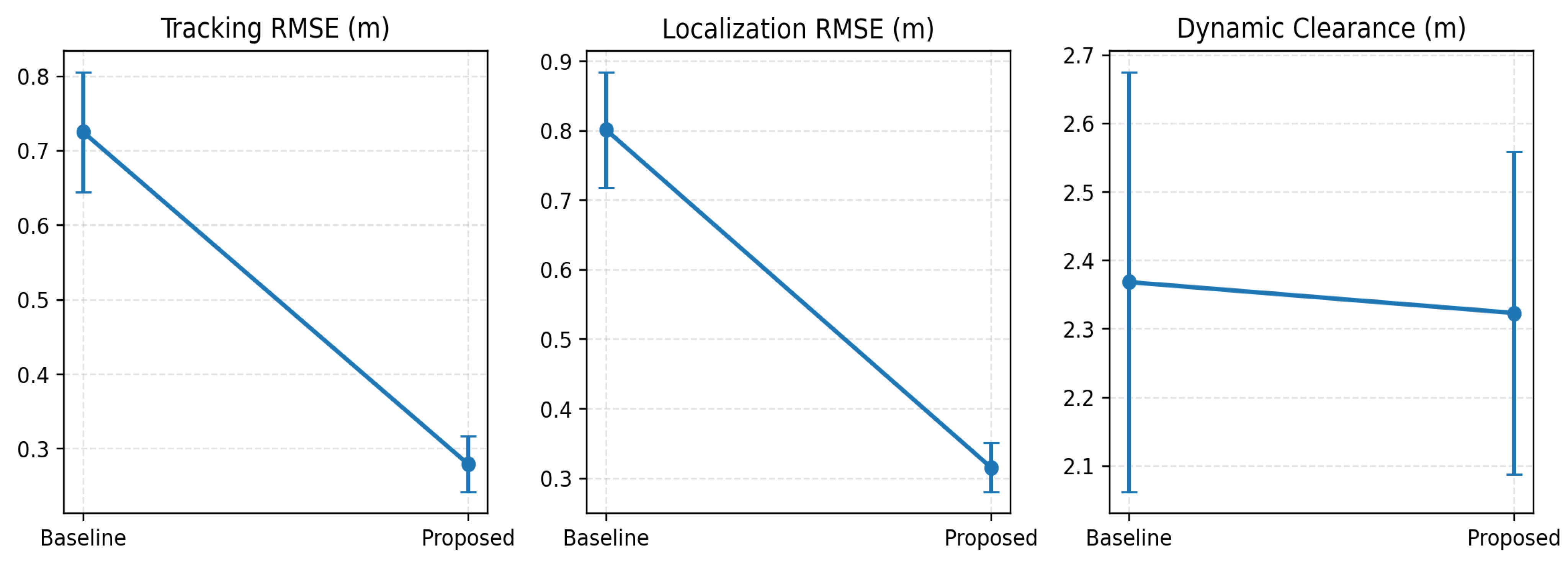
Figure 1. Integrated tracked chassis platform.
Agriengineering 08 00231 g001
Figure 2. Overall system workflow.
Agriengineering 08 00231 g002
Figure 3. Three-dimensional model of the tracked chassis.
Agriengineering 08 00231 g003
Figure 4. Simplified three-dimensional model of the tracked chassis.
Agriengineering 08 00231 g004
Figure 5. Sensor functions and information flow.
Agriengineering 08 00231 g005
Figure 6. IMU-aided NDT scan-to-map localization process.
Agriengineering 08 00231 g006
Figure 7. Tracking RMSE under different slope conditions.
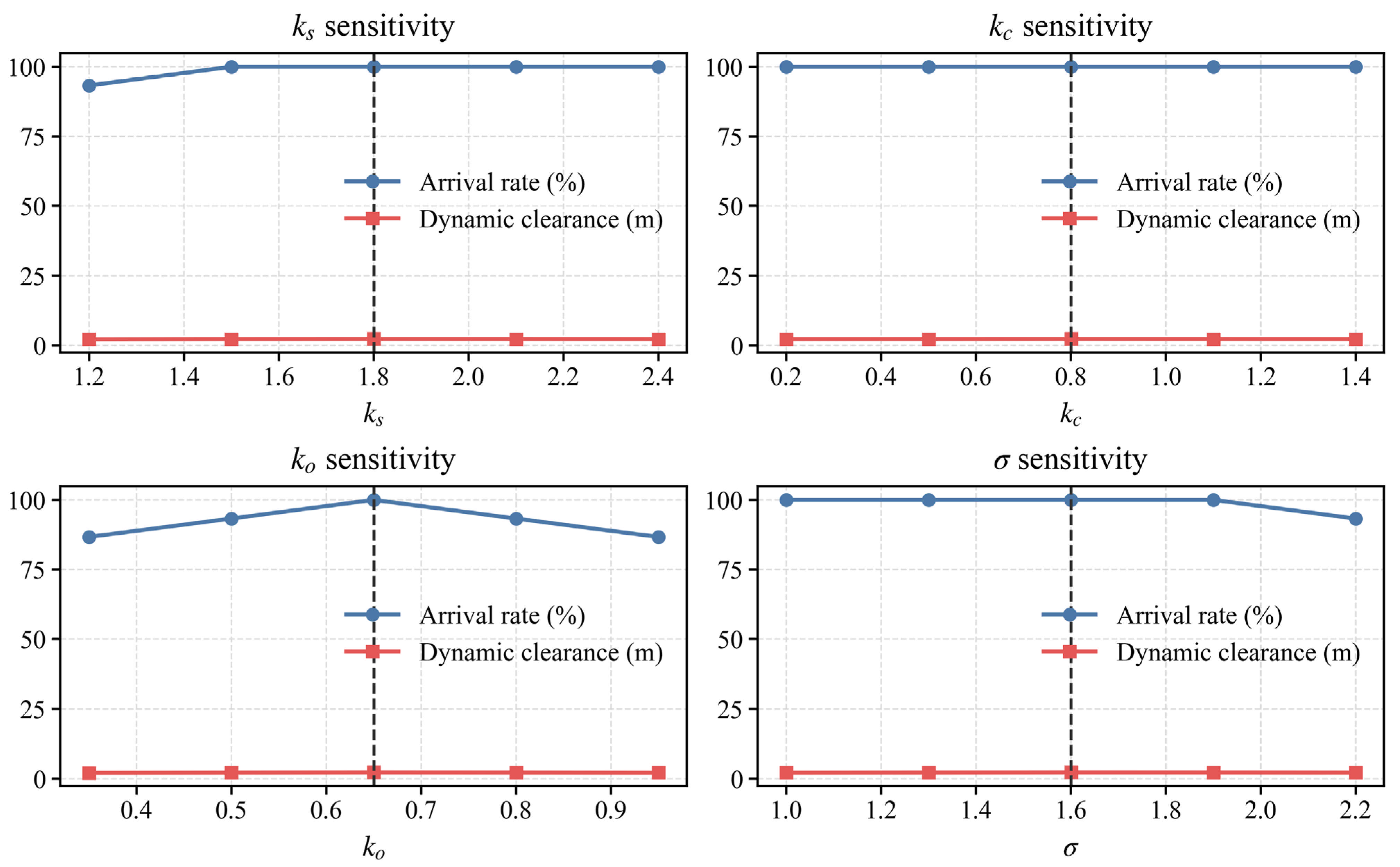
Agriengineering 08 00231 g007
Figure 8. Localization RMSE under different slope conditions.
Agriengineering 08 00231 g008
Figure 9. Minimum dynamic safety clearance under different slope conditions.
Agriengineering 08 00231 g009
Figure 10. Obstacle recall under different slope conditions.
Agriengineering 08 00231 g010
Figure 11. Contribution rates of key modules in the ablation study.
Agriengineering 08 00231 g011
Figure 12. Comparison of heading-rate standard deviation.
Agriengineering 08 00231 g012
Figure 13. Supplementary comparison of resampled curvature variance based on post-processed ROS/Gazebo trajectories.
Agriengineering 08 00231 g013
Figure 14. Comparison of trajectory smoothness index.
Agriengineering 08 00231 g014
Figure 15. Comparison of robust P5 obstacle clearance.
Agriengineering 08 00231 g015
Figure 16. Gazebo/RViz simulation of the baseline algorithm in the simple environment at 25°.
Agriengineering 08 00231 g016
Figure 17. Gazebo/RViz simulation of the proposed algorithm in the simple environment at 25°.
Agriengineering 08 00231 g017
Figure 18. Trajectory comparison in the simple environment at 25°: (a) baseline algorithm; (b) proposed algorithm.
Agriengineering 08 00231 g018
Figure 19. Comparison of point cloud ground segmentation and Euclidean clustering in the simple environment at 25°: (a) baseline algorithm; (b) proposed algorithm.
Agriengineering 08 00231 g019
Figure 20. Gazebo/RViz simulation of the baseline algorithm in the general environment at 20°.
Agriengineering 08 00231 g020
Figure 21. Gazebo/RViz simulation of the proposed algorithm in the general environment at 20°.
Agriengineering 08 00231 g021
Figure 22. Trajectory comparison in the general environment at 20°: (a) baseline algorithm; (b) proposed algorithm.
Agriengineering 08 00231 g022
Figure 23. Comparison of point cloud ground segmentation and Euclidean clustering in the general environment at 20°: (a) baseline algorithm; (b) proposed algorithm.
Agriengineering 08 00231 g023
Figure 24. Gazebo/RViz simulation of the baseline algorithm in the complex environment at 25°.
Agriengineering 08 00231 g024
Figure 25. Gazebo/RViz simulation of the proposed algorithm in the complex environment at 25°.
Agriengineering 08 00231 g025
Figure 26. Trajectory comparison in the complex environment at 25°: (a) baseline algorithm; (b) proposed algorithm.
Agriengineering 08 00231 g026
Figure 27. Comparison of point cloud ground segmentation and Euclidean clustering in the complex environment at 25°: (a) baseline algorithm; (b) proposed algorithm.
Agriengineering 08 00231 g027
Figure 28. Mean values and 95% confidence intervals of repeated Python simulation metrics.
Agriengineering 08 00231 g028
Figure 29. IMU slope-prior robustness under nominal, vibration, drift, and dynamic-motion perturbations.
Agriengineering 08 00231 g029
Figure 30. One-at-a-time sensitivity analysis of the path-planning weights.
Agriengineering 08 00231 g030
Figure 31. Comparison of the proposed method with the original and stronger baselines.
Agriengineering 08 00231 g031
Figure 32. Robustness comparison under mixed perturbations.
Agriengineering 08 00231 g032
Figure 33. Isolated no-LakiBeam1L ablation comparison.
Agriengineering 08 00231 g033
Table 1. Main parameters of the tracked chassis.
ParameterValue
Overall dimensions1415 mm × 945 mm × 518 mm
Suspension typeFour-channel composite damping suspension
Maximum obsta-cle-crossing height200 mm
Maximum trench-crossing capability400 mm; vertical 200 mm/horizontal 250 mm
Operating speed0–5.4 km/h
Track width150 mm
Rated load capacity300 kg
Maximum climbing capability≤30°
Table 2. Sensor configuration and functions.
SensorMain SpecificationFunction
Leishen C16 mechanical LiDARWavelength: 905 nm; ranging accuracy: ±3 cm; ranging precision: ±1 cm (1σ); weight: 1040 g; size: Φ102 mm × 77.9 mmThree-dimensional point cloud acquisition and two-dimensional scanning
Nine-axis IMURoll accuracy: 0.1°; roll range: ±180°; pitch accuracy: 0.1°; pitch range: ±90°Attitude estimation and slope prior
LakiBeam1L single-line LiDARWavelength: 940 nm; measurement accuracy: ±2 cm; detection range: ≥40 m at 70% reflectivity and ≥20 m at 10% reflectivity; size: 60 mm × 60 mm × 80 mm; weight: 160 gDynamic obstacle detection
Table 3. System-level information flow from IMU priors to navigation metrics.
Input InformationIntermediate ComputationAffected ModuleExpected Metric Effect
IMU roll/pitchEquivalent slope angleAdaptive Ray Ground Filter thresholdObstacle recall and clustering precision
IMU roll/pitch/headingPoint cloud attitude compensation and NDT initial poseNDT scan-to-map localizationLocalization RMSE
IMU slope and headingSlope and cross-slope risk costDijkstra/A* path planningPath safety and collision exposure
IMU slope and heading errorSlope-curvature velocity ratioPure Pursuit trackingTracking RMSE and dynamic clearance
Table 4. Key parameter settings and descriptions.
ParameterDescriptionValueBasis
k s Slope risk weight1.8Preliminary tuning in the simple environment and validation in the general and complex environments
k c Cross-slope risk weight0.8Preliminary tuning in the simple environment and validation in the general and complex environments
k o Obstacle potential weight0.65Balances safety clearance and path length
σ Potential-field attenuation parameter1.6 mControls the influence range of obstacles
L 0 Basic look-ahead distance0.9 mControls path-tracking sensitivity
α l i m Slope risk normalization upper limit30°Determined by the safe climbing capability of the chassis
α 0 Initial slope threshold for velocity reductionMaintains normal velocity on mild slopes and gradually reduces velocity above this threshold
s m i n Minimum velocity ratio near the maximum slope0.45Limits velocity on steep slopes to reduce sideslip and trajectory oscillation
k v Velocity gain for look-ahead distance0.85 sAllows the look-ahead distance to vary with velocity
k γ Heading error velocity regulation coefficient0.35   r a d 1 Improves turning stability on sloped terrain
v m a x Maximum linear velocity1.10 m/sConsistent with chassis velocity capability and simulation scale
v m i n Minimum linear velocity0.16 m/sAvoids stagnation or control discontinuity during low-speed tracking
ω m a x Maximum angular velocity1.35 rad/sLimits sharp turning and improves control stability
D 0 Basic safety distance1.35 mDefines the basic near-field obstacle safety margin
T r System response time0.3 sRepresents perception, planning, and control update delay
a d e c Allowable deceleration0.6 m/s2Used to calculate the velocity-dependent dynamic safety distance
r b Equivalent safety radius of the chassis0.45 mConservatively determined according to chassis dimensions and safety envelope
Δ α Local terrain undulation marginCompensates for surface micro-undulation and sensor noise
α m i n Lower bound of the ground-segmentation thresholdPrevents overly strict segmentation under small-slope conditions
α m a x Upper bound of the ground-segmentation threshold32°Prevents low obstacles from being incorrectly merged into ground points under large-slope conditions
ε Small value for avoiding division by zero 1 × 10 3 mEnsures numerical stability in Equation (11)
s γ , m i n Minimum velocity ratio under heading error constraints0.32Avoids excessive deceleration or stagnation during sharp turning
r d y n Equivalent radius of the dynamic obstacle0.45 mUsed for dynamic obstacle inflation and safety distance calculation
m d y n Dynamic safety margin0.85 mCompensates for tracking error and perception uncertainty during dynamic avoidance
β m a x Half-angle of the forward detection sector42°Defines the near-field triggering region
Table 5. Average performance metrics under three environments and five slope conditions.
EnvironmentAlgorithmArrival Rate (%)Collision Rate (%)Tracking RMSE (m)Localization RMSE (m)Dynamic Safety Clearance (m)Obstacle Recall (%)Clustering Precision (%)
ComplexBaseline20.080.00.3730.4251.21479.3582.83
ComplexProposed100.00.00.1800.2132.00298.5198.66
GeneralBaseline40.060.00.3790.5010.47186.1182.74
GeneralProposed100.00.00.2530.2511.68399.0198.44
SimpleBaseline40.040.00.9221.0522.50076.8964.36
SimpleProposed100.00.00.2210.3763.23798.4398.65
Table 6. Average improvement rates of the proposed algorithm relative to the baseline algorithm.
EnvironmentTracking RMSE Reduction (%)Localization RMSE Reduction (%)Dynamic Safety Clearance Improvement (%)Obstacle Recall Improvement (%)Clustering Precision Improvement (%)
Complex51.7449.8864.9124.1519.11
General33.2449.90257.3214.9818.98
Simple76.0364.2629.4828.0153.28
Table 7. Average performance metrics of the ablation study.
AlgorithmArrival Rate (%)Collision Rate (%)Tracking RMSE (m)Localization RMSE (m)Dynamic Safety Clearance (m)Obstacle Recall (%)Clustering Precision (%)
Complete proposed algorithm100.00.00.2180.2802.30898.6598.58
Without IMU-adaptive ground segmentation100.00.00.2180.2802.30887.5180.33
Without slope-aware path cost86.713.30.2800.3232.26597.7397.43
Without slope-adaptive velocity regulation100.00.00.2300.3581.63098.5298.32
Table 8. Average contribution rates of the complete proposed algorithm relative to ablation versions.
Removed ModuleTracking RMSE Reduction (%)Localization RMSE Reduction (%)Dynamic Safety Clearance Improvement (%)Obstacle Recall Improvement (%)Clustering Precision Improvement (%)
IMU-adaptive ground segmentation0.000.000.0012.7322.72
Slope-aware path cost22.1413.311.900.941.18
Slope-adaptive velocity regulation5.2221.7941.600.130.26
Table 9. Raw simulation metrics of representative ROS/Gazebo scenarios.
EnvironmentSlopeAlgorithmReached GoalCollisionRunning Time (s)Path Length (m)Heading-Rate Standard DeviationTrajectory Smoothness IndexP5 Obstacle Clearance (m)
Simple25°BaselineYesNo4.02531.0610.409217.20890.8282
Simple25°ProposedYesNo8.99531.2650.07301.64891.0166
General20°BaselineYesNo3.85031.3131.823374.25370.4539
General20°ProposedYesNo24.57031.4370.09710.95090.5713
Complex25°BaselineYesNo4.13032.7872.7714112.56790.4489
Complex25°ProposedYesNo8.85532.9220.866631.82260.5685
Table 10. Scenario-wise improvement rates of the proposed algorithm relative to the baseline algorithm based on the raw metrics in Table 9.
MetricSimple 25° Improvement (%)General 20° Improvement (%)Complex 25° Improvement (%)Baseline MeanProposed
Mean
Mean Scenario-Wise
Improvement (%)
Heading-rate standard deviation (rad/s)82.1794.6768.731.66800.345681.86
Trajectory smoothness index (rad/s2)90.4298.7271.7368.010211.474286.96
Robust obstacle clearance P5 (m)22.7525.8626.630.57700.718825.08
Table 11. Multi-seed repeated-trial statistics of the Python simulation results.
AlgorithmArrival Rate (%)Collision Rate (%)Tracking RMSE (m)Localization RMSE (m)Dynamic Clearance (m)Obstacle Recall (%)Cluster Precision (%)
Baseline23.3 ± 42.474.7 ± 43.60.725 ± 0.5020.802 ± 0.5182.369 ± 1.91577.74 ± 18.5272.46 ± 23.24
Proposed94.7 ± 22.55.3 ± 22.50.280 ± 0.2330.316 ± 0.2202.324 ± 1.47298.20 ± 3.1397.92 ± 2.75
Table 12. Robustness of the IMU-derived slope prior under simulated perturbations.
ConditionSlope RMSE (°)Slope MAE (°)P95 Abs. Error (°)Obstacle Recall (%)Cluster Precision (%)
Nominal0.245 ± 0.0240.198 ± 0.0230.462 ± 0.06198.93 ± 0.9198.82 ± 0.64
Vibration0.687 ± 0.0780.561 ± 0.0671.259 ± 0.16598.85 ± 0.9898.73 ± 0.74
Drift0.290 ± 0.0570.235 ± 0.0530.549 ± 0.10898.79 ± 0.8998.76 ± 0.65
Dynamic0.815 ± 0.0800.675 ± 0.0741.477 ± 0.16398.88 ± 0.9398.67 ± 0.73
Table 13. One-at-a-time sensitivity summary of the path-planning weights.
ParameterStable IntervalSelected ValueArrival Rate (%)Tracking RMSE (m)Dynamic Clearance (m)Interpretation
k s 1.50–2.401.80100.00.2182.308Below 1.5, arrival rate decreased; 1.8 was kept near the left edge of the stable plateau.
k c 0.20–1.400.80100.00.2182.308The current slope field produced negligible topology changes over 0.2–1.4, so 0.8 was retained as a midrange value.
k o Single feasible value in tested range0.65100.00.2182.308Values below or above 0.65 reduced arrival rate; 0.65 was the center of the feasible region.
σ 1.00–1.901.60100.00.2182.3081.0–1.9 remained feasible; 1.6 was kept as a balance between clearance and tracking smoothness.
Table 14. Stronger baseline comparison on the repeated Python simulation dataset.
AlgorithmArrival Rate (%)Collision Rate (%)Tracking RMSE (m)Localization RMSE (m)Dynamic Clearance (m)
Baseline23.3 ± 42.474.7 ± 43.60.725 ± 0.5020.802 ± 0.5182.369 ± 1.915
Proposed94.7 ± 22.55.3 ± 22.50.280 ± 0.2330.316 ± 0.2202.324 ± 1.472
NDT-ICP + A* + PP65.3 ± 47.834.7 ± 47.80.227 ± 0.1090.372 ± 0.1350.809 ± 0.902
NDT-ICP + A* + DWA89.3 ± 31.08.0 ± 27.20.356 ± 0.1470.341 ± 0.1431.454 ± 0.643
Table 15. Mixed perturbation stress-test statistics.
AlgorithmArrival Rate (%)Collision Rate (%)Tracking RMSE (m)Localization RMSE (m)Dynamic Clearance (m)Obstacle Recall (%)
Baseline29.3 ± 45.870.7 ± 45.80.617 ± 0.5430.693 ± 0.5611.938 ± 2.13184.58 ± 15.36
Proposed81.3 ± 39.218.7 ± 39.20.278 ± 0.1340.290 ± 0.1202.338 ± 1.60098.13 ± 2.80
Table 16. Isolated no-LakiBeam1L ablation results.
AlgorithmArrival Rate (%)Collision Rate (%)Tracking RMSE (m)Localization RMSE (m)Dynamic Clearance (m)
Proposed90.7 ± 29.39.3 ± 29.30.247 ± 0.1050.294 ± 0.1192.322 ± 1.459
Without LakiBeam1L76.0 ± 43.024.0 ± 43.00.215 ± 0.1040.295 ± 0.1211.982 ± 1.764
Table 17. Algorithmic latency benchmark between the LakiBeam1L trigger and the C16 point cloud clustering pipeline.
PipelineMean Latency (ms)Median Latency (ms)Maximum Latency (ms)Interpretation
LakiBeam1L trigger0.01760.01490.1467Direct distance-bearing safety decision
C16 scan + RGF + clustering12.252711.643529.8980Full point cloud generation, segmentation, clustering, and matching
Table 18. Statistical tests for the repeated Python simulation dataset.
MetricBaseline MeanProposed MeanWelch Test pMann–Whitney U/Fisher Exact Test p
tracking_rmse_m0.7250.2804.05 × 10−193.29 × 10⁻³²
localization_rmse_m0.8020.3164.42 × 10−212.65 × 10⁻³²
min_dynamic_clearance_m2.3692.3240.81910.6629
obstacle_recall_pct77.74098.1981.21 × 10−271.04 × 10⁻³⁵
cluster_precision_pct72.45597.9152.18 × 10−279.51 × 10⁻³³
goal_reached0.2330.947 2.81 × 10−40
collision0.7470.053 2.60 × 10−38
Disclaimer/Publisher’s Note: The statements, opinions and data contained in all publications are solely those of the individual author(s) and contributor(s) and not of MDPI and/or the editor(s). MDPI and/or the editor(s) disclaim responsibility for any injury to people or property resulting from any ideas, methods, instructions or products referred to in the content.