Article

A Comparative Study on Rice Diversity Mapping with PlanetScope and Sentinel-2 Red Edge Bands Based on Key Phenological Characteristics

1
Geological Survey of Jiangsu Province, Nanjing 210018, China
2
Jiangsu Provincial Satellite Application Technology Center for Natural Resources, Nanjing 210018, China
3
Jiangsu Provincial Key Laboratory of Satellite Remote Sensing Applications, Nanjing 210018, China
4
Xinyi Natural Resources and Planning Bureau, Lianyungang 221499, China
*
Author to whom correspondence should be addressed.
AgriEngineering 2026, 8(5), 187; https://doi.org/10.3390/agriengineering8050187
Submission received: 4 March 2026 / Revised: 26 April 2026 / Accepted: 28 April 2026 / Published: 10 May 2026

Highlights

What are the main findings?
  • Classification accuracy for rice varieties peaks consistently at the Heading–Flowering stage for both PlanetScope and Sentinel-2, indicating phenology as the dominant control factor.
  • A single red-edge band from PlanetScope provides classification performance comparable to Sentinel-1 multi-red-edge configurations, while delivering clearer field-scale spatial delineation.
What are the implications of the main findings?
  • Increasing the number of red-edge bands does not guarantee proportional gains in variety-level crop mapping; effective performance depends on the synergy among phenology, spatial resolution, and key spectral features.
  • High-resolution imagery with essential red-edge information can serve as a practical alternative for fine-scale crop variety monitoring in fragmented agricultural landscapes.

Abstract

Precise mapping of rice cultivars is of great significance for crop management and food security evaluation. Nevertheless, differentiating between Indica and Japonica rice remains a formidable task, mainly due to subtle discrepancies in spectral characteristics and scattered planting distributions. This study evaluated the synergistic effect of spatial resolution and red edge information in rice variety classification using PlanetScope (PS) and Sentinel-2 (S2) images from the Tillering and Jointing stage, Heading and Flowering stage in Huai’an, Jiangsu Province. Multiple feature schemes were constructed, including spectral bands, vegetation indices, and texture features, with and without red-edge variables. A total of eight feature schemes have been constructed, including spectral bands, vegetation index, texture features, and red edge features. The feature scheme division is based on the participation of different sensors, growth periods, and red edges. We fine-tune three classification models, Random Forest (RF), Light Gradient Boosting Machine (LightGBM), and TabNet, to enhance classification performance. Additionally, we employ Shapley Additive Explanations (SHAP) to quantitatively measure the contribution of each feature to the prediction of distinct rice varieties. Results demonstrate that classification accuracy of different sensors reach the highest at the Heading and Flowering stage. The overall accuracy of PS scheme is 98.14%, the F1 scores of Japonica and Indica rice are 97.67% and 98.41%, the overall accuracy of S2 scheme is 97.87%, and the F1 scores of Japonica and Indica rice are 98.62% and 98.68, respectively. Incorporating red-edge features leads to a notable improvement in F1-scores for both Indica and Japonica rice under all experimental configurations. Although PS only has one red edge band set, its classification performance is similar to S2, and the boundaries between different rice variety recognition results and between non rice and rice plots are more refined compared to S2. Feature attribution analysis reveals that red-edge indices exert a dominant influence on the decision-making process of the models, especially during the Heading–Flowering period. These findings suggest that high-accuracy discrimination of rice varieties relies heavily on the synergistic optimization of phenological timing, red-edge spectral information, and spatial resolution, rather than merely increasing spectral dimensionality. The optimization direction for high-precision rice variety mapping in the future should prioritize the collaborative mechanism of phenological period, red edge data, and spatial resolution, rather than being limited to simple stacking in the spectral dimension.

1. Introduction

As one of the world’s most indispensable staple food crops, rice directly and profoundly influences food security evaluation, the optimization of agricultural planting systems, and the deployment of precision farming practices through its planting scale, yield output, and cultivar composition [1,2]. With the rapid advancement and widespread adoption of remote sensing technology in agricultural, rice remote sensing mapping has advanced beyond conventional crop type recognition to the more sophisticated demand of fine-grained cultivar-level differentiation [3]. Distinguishing between different rice cultivars (e.g., Indica and Japonica rice) within the same species poses a far greater challenge than separating rice from other crop types. This challenge arises from their subtle variations in physiological traits, phenological development dynamics, and yield formation mechanisms [4]. Nonetheless, such fine-scale cultivar discrimination is vital for evidence-based agricultural decision-making, dynamic monitoring of rice cultivar structures, and regional food productivity assessment [5]. As a result, remote sensing-based identification of rice at the cultivar level remains a prominent challenge, mainly due to highly fragmented rice planting patterns and minimal spectral variations between different rice cultivars.
In recent decades, the rapid development of optical remote sensing imagery with high spatiotemporal resolution has provided a novel technical foundation for fine-scale crop classification and mapping [6]. Notably, the red-edge band, which is highly sensitive to changes in vegetation chlorophyII content, nitrogen nutritional status, and canopy structural properties, has been widely applied in crop growth monitoring, vegetation condition evaluation, and crop type identification [7,8,9]. Abundant research confirms that integrating red-edge spectral information can effectively improve the accuracy of crop classification and biophysical parameter retrieval, with particularly strong improvement during the middle and late phases of crop growth [10,11]. However, most existing studies focus on the binary question of whether to use red-edge information. Few studies explore how variations in red-edge configurations) affect cultivar-level crop identification [12]. The red edge band shows significant advantages in distinguishing different crop types such as corn, wheat, and rice, but there is relatively little research on the precise identification of different varieties within crop types. Compared to crop type recognition that relies on significant phenotypic differences, variety level recognition faces smaller spectral differences and more complex spatial distributions, which puts higher demands on the sensitivity of red edge information. At present, most studies focus on the overall contribution of the red edge band to the classification accuracy, and relatively few studies focus on the red edge utility of the variety recognition level and the impact of different sensor red edge configurations.
Moreover, remote sensing-based crop identification strongly responds to crop growth phenological stages [13]. Changes in canopy structure, pigment content, and physiological status across different growth stages directly affect spectral response characteristics [14]. Existing research shows that Tillering, Jointing, Heading, and Flowering stages in the middle and later stages of rice growth are the key stages of high rice recognition accuracy [15]. However, under different sensor conditions, whether the importance of phenology on variety differentiation is consistent, and whether the role of red edge information in different growth stages is significantly different, still lacks targeted analysis. Notably, the synergistic effects between crop phenology and spectral configurations among sensors with distinct spatial resolutions and spectral characteristics have not yet been fully clarified [16].
Against this backdrop, systematically investigating the synergistic mechanisms of red-edge spectral information, crop phenological stages, and sensor attributes in rice cultivar identification has become a key scientific problem in advancing refined agricultural remote sensing applications. Based on the above considerations, this study selects a typical rice-cultivating region as the research area and uses optical imagery from PS and S2 to conduct a systematic comparative study on remote sensing identification of Indica and Japonica rice cultivars. By constructing diverse classification scenarios based on different growth stages and feature combinations, this research clarifies the differences and synergistic mechanisms between red-edge spectral information and spatial resolution in identifying rice cultivars. To verify that PS data with only a single red edge band can be comparable to S2 with multiple red edge bands in rice variety recognition ability, and to explore the improvement effect of high spatial resolution red edge information on recognition results, the following specific objectives are set in this study: (1) To compare the classification performance of PS and S2 imagery, and analyze the overall capacity of the two sensors for rice cultivar mapping under different sensor conditions. (2) To evaluate the impact of red-edge information on rice cultivar identification at different phenological stages, and identify the critical growth periods most sensitive to rice cultivar discrimination. (3) To explore the differences in identification effectiveness between the single red-edge band of PS and the multi-red-edge band configuration of S2, and verify whether increasing the number of red-edge bands can stably improve the accuracy of rice cultivar identification. This study aims to provide a scientific basis for the rational selection of multi-source remote sensing imagery and efficient utilization of red-edge spectral information in rice cultivar identification, while also offering a methodological reference for applying high-spatial-resolution remote sensing data in precision agricultural mapping.

2. Materials and Methods

2.1. Study Area

The research area is located in Huai’an City, a typical rice-growing region on the Jianghuai Plain. Geographically, this area features flat terrain and an extensive, interconnected water network of rivers and lakes (Figure 1). The region has a subtropical monsoon climate, with an annual average temperature of 15.1 °C and mean annual precipitation of approximately 993 mm. Rice is the dominant staple food crop in Huai’an, with a total cultivation area of 324,000 hectares. Driven by large-scale promotion of ecological integrated farming models such as rice-shrimp and rice-crab polyculture, the planting area of Indica rice in the region now accounts for more than one-third of the total rice planting area, while Japonica rice constitutes the majority of the remaining cultivation area. A representative subregion in central Huai’an, where Japonica and Indica rice grow in a fragmented pattern, was selected as the core study area. The high level of land fragmentation and the synchronous growth of different rice varieties in this subregion pose considerable challenges for remote sensing-based rice variety discrimination (Figure 2), requiring remote sensing data with high spatial and spectral resolution to ensure accurate identification [17].

2.2. Data and Processing

2.2.1. Satellite Imagery

The satellite remote sensing datasets include PS and S2 imagery, two of the limited multispectral satellite data sources that integrate red-edge spectral bands into their observation systems [18,19]. To enable rigorous and comparable analysis between the two sensors, strict consistency was maintained across all datasets in terms of image acquisition time windows, preprocessing workflows, and remote sensing feature extraction protocols. The PS data used in this study are Level-3B surface reflectance (SR) products, whereas S2 data are Level-2A SR products. Both datasets undergo standardized preprocessing pipeline including radiometric calibration, high-precision geometric correction, and atmospheric correction. Specifically, the S2 data are SR products with 10 m spatial resolution, acquired on 29 July 2024 and 27 September 2024 from the Copernicus Data Space Ecosystem (CDES) via its official platform (https://dataspace.copernicus.eu). In comparison, the PS data are SR products with 3 m high spatial resolution, acquired on 31 July 2024 and 28 September 2024 through procurement. Detailed spectral band settings and spatial resolution parameters of the PS and S2 sensors are presented in Table 1.
Since the spectral bands of PS are concentrated in the visible to near-infrared (VNIR) spectrum, while those of S2 span the visible, near-infrared, and shortwave infrared (VNIR-SWIR) regions, we select the overlapping VNIR spectrum for this study to ensure data comparability (Table 1). This selection specifically includes Bands 1–8 of PS and Bands 1–9 of S2. PS images maintain their original 3 m spatial resolution, while S2 images are resampled to a 10 m spatial resolution using bilinear interpolation.

2.2.2. Sample Data

We collect ground truth sample data through a combination of field surveys and visual interpretation of high-resolution Google Earth imagery. To ensure an adequate number of pixels for model training and validation while maintaining pixel purity, samples were delineated as polygons [20]. The selection criteria focus on areas with consistent land cover types and far from the boundaries of different land cover types. Considering local land surface characteristics, we identify seven primary land cover categories comprising a total of 405 samples: Building (51), Water (34), Forest (45), Greenhouse (33), Japonica rice (90), Indica rice (109), and Lotus pond (43). We use a stratified sampling strategy to randomly select 50% of the samples for model training, while reserving the remaining 50% for independent accuracy assessment [21].

2.3. Methods

2.3.1. General Technical Workflow

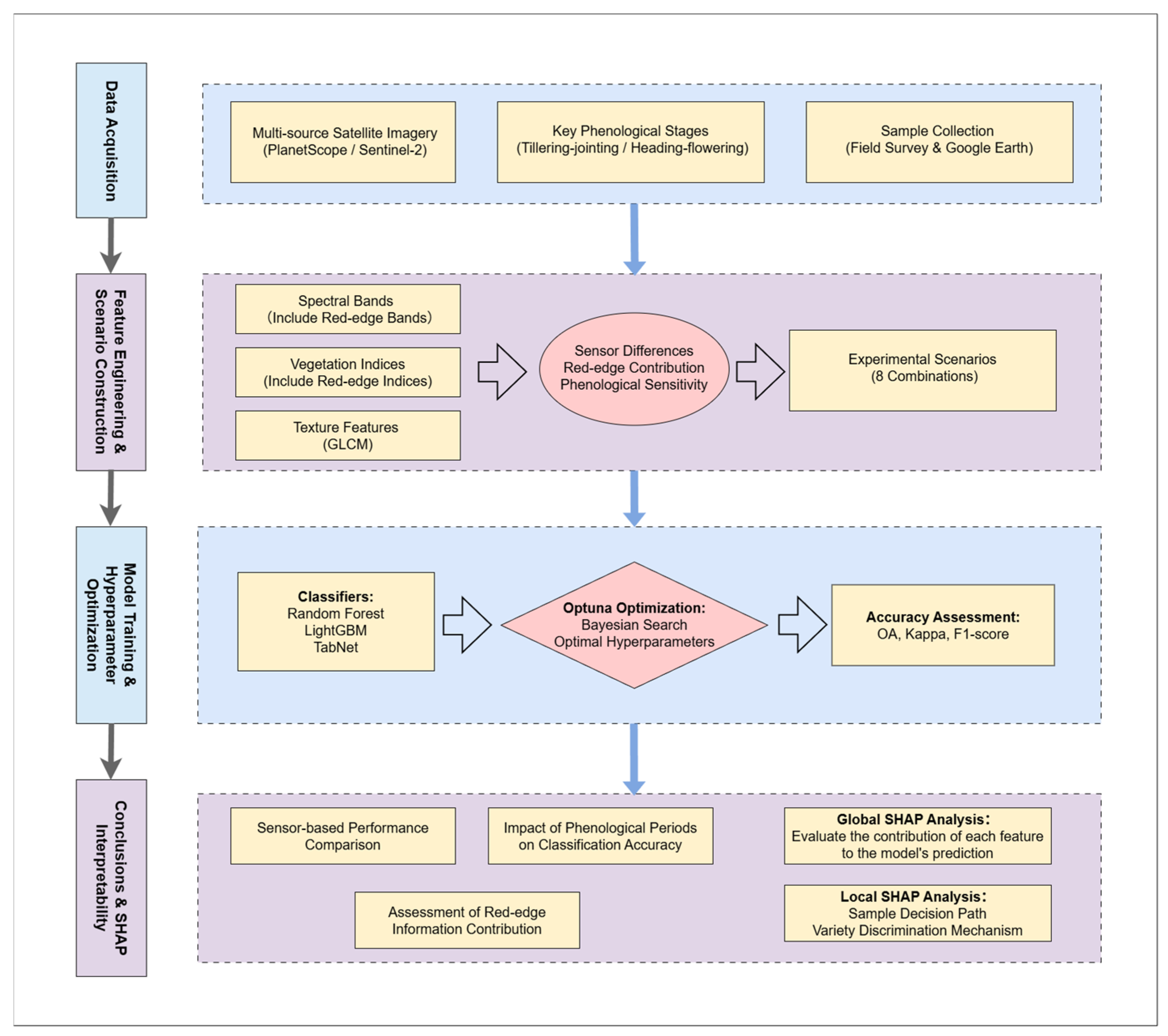
The technical workflow in this study includes four core sequential stages: feature extraction, experimental scenario construction, classification model development, and result analysis and interpretation. First, we extract spectral reflectance bands, vegetation spectral indices, and spatial texture features from PS and S2 imagery corresponding to the two key rice phenological stages, to build a comprehensive multi-dimensional remote sensing feature dataset for subsequent modeling. On the basis of this integrated dataset, we design eight distinct experimental scenarios by stratifying according to three variables: rice phenological stage, remote sensing sensor type, and red-edge information inclusion status. We construct these scenarios to quantitatively evaluate the individual and interactive impacts of phenological timing, sensor-specific characteristics, and red-edge spectral information enhancement on the accuracy of rice variety remote sensing identification.
To eliminate bias caused by performance differences among classification algorithms, we select three models, RF, LightGBM, and TabNet for parallel model training and identification accuracy assessment. The Optuna hyperparameter optimization framework was applied to all three models to search for their optimal parameter combinations, ensuring rigorous and objective evaluation of rice variety identification performance across all experimental scenarios. After determining the optimal classification model for each scenario, we further use the SHAP framework to quantitatively measure the global contribution of each remote sensing feature to the discrimination of japonica and indica rice. In addition, a sample-level local interpretability analysis was conducted on representative Japonica and Indica rice samples using the SHAP method, to explore specific feature contribution paths underlying the model’s prediction decisions for individual rice variety samples. The complete technical implementation roadmap of this study is presented in Figure 3.

2.3.2. Feature Extraction

To fully exploit the information from PS and S2 data and improve identification of different rice varieties, we construct a multi-dimensional feature set by extracting spectral bands, vegetation indices, and texture features.
Spectral bands and indices mainly capture spectral discrepancies between rice varieties and different land cover types, while texture features characterize spatial structures [22]. For spectral band features, all bands within the VNIR spectrum were used as input, specifically Band 1–8 for PS and Band 1–9 for S2. For index features, we select vegetation indices widely demonstrated to be sensitive to crop physiology and structure and to show superior performance in crop classification, such as the Normalized Difference Vegetation Index (NDVI), Enhanced Vegetation Index (EVI), Normalized Difference Red Edge (NDRE), and MERIS Terrestrial ChlorophyII Index (MTCI) [23,24,25], as presented in Table 2.
We extract texture features using the Gray-Level Co-occurrence Matrix (GLCM) [26]. To generate grayscale images for GLCM computation, a linear combination of the blue, green, and red bands was employed. Compared with calculating the GLCM for each band individually, this linear combination preserves spatial information while effectively reducing data redundancy [27]. The formula for calculating the grayscale image used in the GLCM is as follows:
G r a y = R × 0.31 + G × 0.58 + B × 0.11
where R, G, and B represent the red, green, and blue bands, respectively.
We use 3 × 3 sliding window to calculate the GLCM across four directions (0°, 45°, 90°, and 135°), and average the results to obtain final texture values [28]. At this window size, it is possible to preserve the boundaries of land features to the greatest extent possible and suppress mixed pixel pollution caused by the edge blurring effect [29]. Given the correlation between different texture measures, eight metrics that effectively characterize spatial heterogeneity were selected: Mean, Variance, Homogeneity, Contrast, Dissimilarity, Entropy, Second-Moment, and Correlation [30,31].
Table 2. Categorization and detailed configuration of the extracted feature sets.
Data TypeFeature TypeContentFormula
PlanetScopeSpectral bandsB1, B2, B3, B4, B5, B6, B8 N D V I = ( B 8 B 6 ) ( B 8 + B 6 )
W D R V I = ( 0.2 × B 8 B 6 ) ( 0.2 × B 8 + B 6 )
E V I = 2.5 ( B 8 B 6 ) ( B 8 + 6 × B 6 7.5 × B 2 + 1 )
G N D V I = ( B 8 B 4 ) ( B 8 + B 4 )
S A V I = ( ( B 8 B 6 ) × 1.5 ) ( ( B 8 + B 6 ) + 0.5 )
N D R E = ( B 8 B 7 ) ( B 8 + B 7 )
P S R I = ( B 8 B 2 ) B 7
M T C I = ( B 7 B 6 ) ( B 7 + B 6 )
N D Y V I = ( B 8 ( B 7 + B 5 ) ( B 8 + ( B 7 + B 5 )
N D G I = ( B 3 B 4 ) ( B 3 + B 4 )
Red-edge spectral bandB7
Vegetation indicesNDVI, EVI, GNDVI, NDGI, NDYVI, SAVI, WDRVI [32,33,34]
Red-edge vegetation indicesMTCI, NDRE, PSRI [24,32]
Texture featuresMean, Variance, Homogeneity, Contrast, Dissimilarity, Entropy, SecondMoment, Correlation
Sentinel-2Spectral bandsB1, B2, B3, B4, B8, B8A N D V I = ( B 8 B 4 ) ( B 8 + B 4 )
E V I = 2.5 ( B 8 B 4 ) ( B 8 + 6 × B 4 7.5 × B 2 + 1 )
G N D V I = ( B 8 B 3 ) ( B 8 + B 3 )
S A V I = ( ( B 8 B 4 ) × 1.5 ) ( ( B 8 + B 4 ) + 0.5 )
W D R V I = ( 0.2 × B 8 B 4 ) ( 0.2 × B 8 + B 4 )
N D R E = ( B 8 B 5 ) ( B 8 + B 5 )
M T C I = ( B 6 B 5 ) ( B 5 + B 4 )
P S R I = ( B 8 B 2 ) B 5
R E P I = 700 + 40 ( B 4 + B 6 2 B 5 ) ( B 6 B 5 )
C l r e = ( B 7 B 5 ) 1
Red-edge spectral bandB5, B6, B7
Vegetation indicesNDVI, EVI, GNDVI, SAVI, WDRVI [32,33,34]
Red-edge vegetation indicesNDRE, MTCI, Cire, PSRI [24,32], REPI [33,35]
Texture featuresMean, Variance, Homogeneity, Contrast, Dissimilarity, Entropy, SecondMoment, Correlation

2.3.3. Experimental Schemes Design

To systematically evaluate the contribution of red-edge features from PS and S2 imagery to rice variety identification, eight experimental schemes were designed based on three dimensions: sensor type, phenological stage, and feature configuration (Table 3).
We organize the schemes into four comparative groups (Scheme 1-Scheme 2, Scheme 3-Scheme 4, Scheme 5-Scheme 6, and Scheme 7-Scheme 8). Each group includes a baseline scheme and a corresponding red-edge augmented scheme. Baseline schemes consist of a fundamental feature set, including multispectral bands (excluding red-edge), non-red-edge vegetation indices, and GLCM texture features. The second scheme in each group expands the baseline by incorporating red-edge spectral bands and their associated indices. This combinatorial design addresses the following objectives: (1) Red-edge Contribution Analysis: To assess the accuracy gains from red-edge information across different sensors and growth stages; (2) Phenological Sensitivity: to investigate the discriminative power of red-edge features during the Tillering–Jointing versus Heading–Flowering stages. (3) Cross-sensor Evaluation: to compare the efficacy of the single red-edge band configuration of PS against the multi-red-edge band configuration of S2.

2.3.4. Model Construction Methods

We train and validate each experimental scheme across all three algorithms to ensure comprehensive and robust evaluation of model rice variety identification performance [36]. Given the critical impact of hyperparameter settings on model predictive performance, we use the Optuna optimization framework to tune hyperparameters of all three models. This approach eliminates potential biases in feature performance evaluation arising from inconsistent parameter configurations and derives the optimal model structure for each classification algorithm.
(1)
Classification Algorithms
RF is an ensemble learning model built on a cascade of decision trees. The algorithm generates a diverse set of decision trees through random resampling of the training dataset and random selection of feature variables, with the final classification result determined by a majority voting mechanism across all constituent trees. Compared with other machine learning methods, RF shows superior robustness and ease of implementation. It can process high-dimensional input features without prior dimensionality reduction. Additionally, the model provides an unbiased estimation of internal generalization error during training and maintains reliable performance even with missing values in the input dataset [37]. The key hyperparameters we optimize for the RF model include the number of decision trees (n_estimators), the maximum depth of individual trees (max_depth), and the minimum number of samples required to split an internal node (min_samples_split). The search range of the hyperparameter n_estimators is set to 50–300, that of max_depth ranged from 5 to 30, and the interval for min_samples_split is defined as 2–15.
LightGBM is a highly efficient gradient boosting classification model based on the Gradient Boosting Decision Tree (GBDT) framework. By adopting Gradient-based One-Side Sampling (GOSS) and Exclusive Feature Bundling (EFB) optimization strategies, LightGBM achieves high-efficiency parallel training, significantly accelerating computational speed while preserving high classification accuracy. This makes it particularly suitable for processing high-dimensional remote sensing feature data [38]. Due to the model’s inherent sensitivity to overfitting, hyperparameter optimization is essential for its application. We tune four core hyperparameters to maximize LightGBM performance: n_estimators, max_depth, the learning rate (learning_rate), and the maximum number of leaves per tree (num_leaves). The hyperparameter search range for n_estimators is set to 50–500; that for learning_rate is specified as 0.01–0.3; the search interval for num_leaves is defined as 20–100; and the corresponding range for max_depth is determined to be 5–12.
TabNet is a deep learning architecture developed by Google Research, specifically engineered for structured data classification tasks. It incorporates a sequential attention mechanism that dynamically adjusts the weight of each input feature during model forward propagation. By mimicking the hierarchical decision-making logic of traditional decision trees, TabNet processes each feature independently before adaptively fusing processed feature information to generate classification predictions. Compared with conventional machine learning models, TabNet demonstrates a stronger ability to extract deep, complex patterns from raw data and delivers excellent performance in intricate land cover classification tasks. Its built-in attention mechanism automatically prioritizes the most discriminative features for the classification task, enhancing learning efficiency, and making it well-suited for uncovering complex non-linear relationships within remote sensing datasets. Given TabNet’s high sensitivity to hyperparameter configurations, we systematically optimize five key parameters to balance model complexity and generalization ability: decision prediction layer dimension (n_d), attention layer dimension (n_a), number of decision steps (n_steps), relaxation factor (gamma), and sparsity regularization coefficient (lambda_sparse). The hyperparameter search range of n_d is set to 8–64, while n_a is constrained to be identical to n_d without independent searching. The search range of n_steps is defined as 3–7, that of γ ranges from 1.1 to 1.8, and the hyperparameter interval of gamma is limited to 1 × 10⁻⁵–1 × 10⁻³. In addition, the batch size of the TabNet model is fixed at 1024, and the number of training epochs is set to 200. The Adam optimizer is adopted for weight updating with an initial learning rate of 0.02. Meanwhile, the early stopping strategy is implemented, with the patience value configured as 30.
(2)
Accuracy Assessment
To validate the overall classification performance of trained models and their specific identification accuracy for Japonica and Indica rice, we construct a confusion matrix using model predictions on the pre-designated independent validation dataset. Four key quantitative evaluation metrics were calculated from the confusion matrix: Overall Accuracy (OA), Kappa coefficient, Japonica rice F1-score, and Indica rice F1-score. The calculation formulas for these metrics are as follows:
O A = i = 1 k N i i N × 100 %
K a p p a = N i = 1 k N i i i = 1 k ( N i + × N + i ) N 2 i = 1 k ( N i + × N + i )
F 1 s c o r e = 2 N i i N + i × N i i N i + N i i N + i + N i i N i + × 100 %
where N represents the total number of samples; k denotes the total number of categories; Nii is the number of samples correctly classified into the i-th category; N+i and Ni+ are the total number of ground truth samples and the total number of predicted samples for the i-th category, respectively.
(3)
Hyperparameter Optimization Framework
Optuna is an automated hyperparameter optimization framework based on Bayesian optimization. Unlike traditional grid search and random search methods that require exhaustive traversal of predefined parameter ranges, Optuna uses the Tree-structured Parzen Estimator (TPE) algorithm to construct a probabilistic proxy model. This approach dynamically guides the sampling direction of subsequent hyperparameters based on historical trials results, enabling rapid identification of sensitive regions for key hyperparameters. The Bayesian optimization strategy employed by Optuna effectively mitigates the risk of local optima and mitigates model overfitting while handling interdependent hyperparameters to ensure logical consistency of parameter combinations [39]. When optimizing the RF, LightGBM and TabNet models via the hyperparameter optimization framework, a single comprehensive objective function was adopted. The optimization target is defined as the average value of the Kappa coefficient and the F1-score for rice samples of different varieties.

2.3.5. SHAP-Based Interpretability Analysis

The SHAP method uses Shapley Value theory from game theory to interpret machine learning models predictive outputs, thereby quantifying the contribution degree of distinct remote sensing features to model prediction results. SHAP assigns a unique contribution value to each input feature, which quantifies the magnitude of the feature’s impact on the deviation between the predictive result of an individual sample and the average prediction of the model across all samples. By delivering accurate local interpretability for single samples and adhering to the consistency principle, SHAP effectively addresses the “black-box” interpretability challenge of machine learning models when processing multi-source, high-dimensional remote sensing datasets [40].
Based on the SHAP framework, this study quantitatively evaluates the global predictive contribution of various remote sensing features to the discrimination of Japonica and Indica rice. Simultaneously, we select representative rice samples to conduct local-level analysis, which explores specific feature contribution paths underlying model predictive decisions for rice variety identification. Global SHAP analysis quantified the overall influence of each feature by calculating mean absolute shapley values across the entire sample set [41]. Local SHAP analysis characterizes the dynamic influence paths of different features on specific representative samples, which vividly illustrates how individual features cumulatively drive the model’s prediction from the baseline value to the final predictive output for a single sample [42]. This analytical process intuitively visualizes the entire decision-making process of the model, from the initial baseline prediction to the final predictive result for individual rice samples.

3. Results

3.1. Classification Accuracy Assessment Under Different Feature Schemes and Sensor Conditions

To systematically evaluate the impact of different sensors, feature configurations, and phenological stages on rice variety identification, this study constructs multiple schemes using PS and S2 data. We perform classification experiments during two critical phenological stages: the Tillering–Jointing stage and the Heading–Flowering stage. The classification performance of each scheme was evaluated using Overall Accuracy (OA), the Kappa coefficient, and F1-scores for both Indica and Japonica rice. The results are summarized in Table 4.

3.1.1. Consistency Analysis of Results Across Different Classifiers

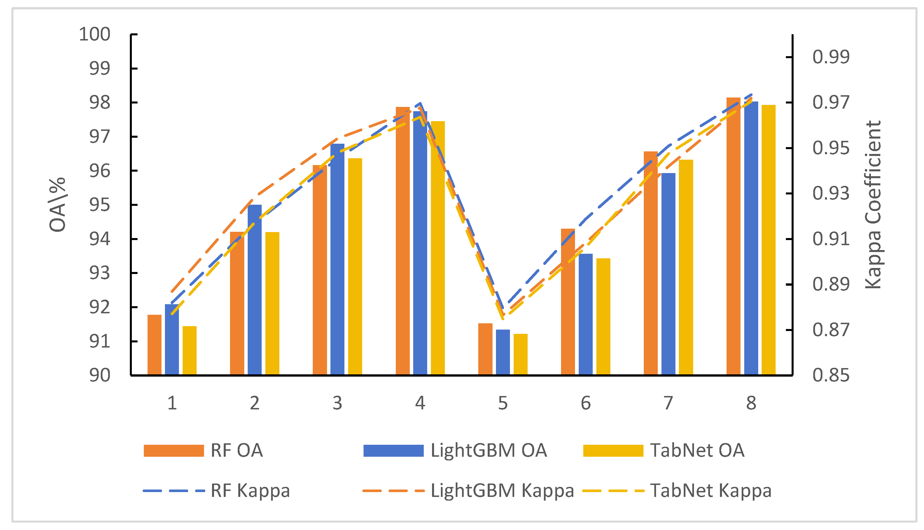
Across all schemes, RF, LightGBM, and TabNet demonstrate a high degree of consistency in classification performance. Fluctuations in OA, Kappa coefficient, and variety-specific F1-scores among different models are relatively minor. Furthermore, accuracy trends corresponding to changes in feature combinations remain consistent across models (Figure 4).
In terms of overall accuracy performance, Scheme 4 and Scheme 8, which incorporate red-edge information, perform best across all models, with OA consistently exceeding 97.45%. Among them, the RF classifier in Scheme 8 achieved the highest accuracy (OA = 98.14%, Kappa = 0.9735). In contrast, baseline schemes without red-edge information (Scheme 1 and Scheme 5) yield relatively lower accuracies, with OA fluctuating between 91.21% and 92.08%.
In terms of model performance, only marginal discrepancies are observed among RF, LightGBM and TabNet. Within each scheme, the OA difference between the best-performing and worst-performing models is generally less than 1%. By contrast, the OA discrepancy between the S2 and PS schemes ranges approximately from 3% to 6%. Specifically, Scheme 2 presents the largest model difference in OA at 0.8%, while Scheme 8 yields the smallest difference of 0.21%. This cross-model stability suggests that, within the context of this study, improvements in rice variety identification performance are primarily driven by input features, rather than the choice of classifier algorithm.

3.1.2. Impact of Red-Edge Features on Identification Accuracy

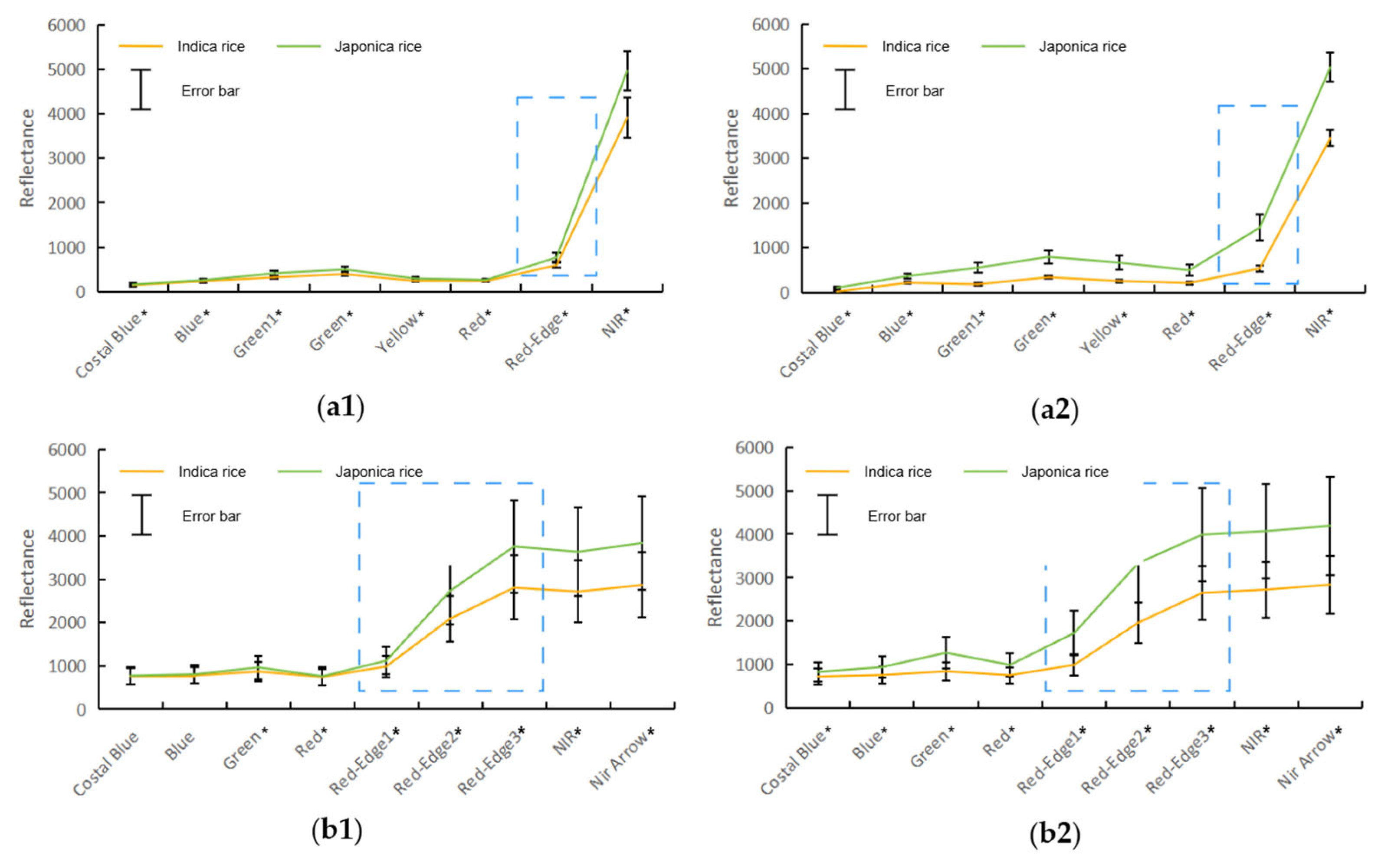
To analyze spectral discrepancies between Japonica and Indica rice, we extract the reflectance of each spectral band from both rice varieties across different phenological stages and datasets, as illustrated in Figure 5. Figure 5(a1,a2) show that the reflectance differences between Japonica and Indica rice in the red-edge and NIR bands of the PS data are more pronounced than in other bands. Furthermore, the reflectance discrepancy in the red-edge band during the Heading–Flowering stage is greater than that during the Tillering–Jointing stage. Figure 5(b1,b2) demonstrate that for S2 data, reflectance differences between the two varieties in the red-edge to NIR spectrum are also more pronounced than in other bands. Similar to PS data, these discrepancies increase notably as rice enters the Heading–Flowering stage.
Under the same sensor and phenological conditions, comparing feature schemes with and without red-edge information reveals that incorporating red-edge features substantially improves rice variety identification.
Specifically, relative to Scheme 1, Scheme 2 shows an average F1-score increase of 3.96% for Japonica rice and 3.28% for Indica rice. Compared to Scheme 3, Scheme 4 achieved increases of 1.16% and 1.02% for Japonica and Indica rice, respectively. Compared to Scheme 5, Scheme 6 resulted in improvements of 3.61% for Japonica and 2.97% for Indica. Finally, compared to Scheme 7, Scheme 8 led to gains of 2.52% for Japonica and 2.65% for Indica.
When comparing results across different phenological stages, for both PS and S2 data, the improvement in identification accuracy attributed to red-edge features during the Tillering–Jointing stage is notably higher than during the Heading–Flowering stage. This suggests that the efficacy of red-edge features is strongly influenced by the phenological stage.

3.1.3. Comparison of Classification Performance Across Different Phenological Stages

From the perspective of phenological stages, classification accuracies obtained by both sensors during the Heading–Flowering stage are consistently higher than those during the Tillering–Jointing stage. This trend remained consistent across all feature schemes, indicating that the phenological stage is a critical factor influencing the remote sensing identification of rice varieties. Particularly during the Heading–Flowering stage, combining red-edge features with conventional spectral and texture features demonstrates superior discriminative power, effectively enhancing the separability of Indica and Japonica rice within the feature space.
Synthesizing results from different sensors and feature schemes, the combination of Heading–Flowering stage with red-edge features shows optimal performance for rice variety identification in this study. Consequently, we base subsequent analysis of feature contributions and underlying mechanisms primarily on data from the Heading–Flowering stage.

3.2. Quantitative Analysis of Feature Contributions Based on SHAP

To further quantify the contribution of different features in the classification decision-making process, this study conducts interpretability analysis of representative classification schemes based on the SHAP method. Considering differences in classification accuracy and results representativeness, SHAP analysis focuses primarily on red-edge schemes at the Heading–Flowering stage, and their corresponding schemes without red-edge features (Table 5). Features extracted during this phenological phase show stronger discriminative ability for Japonica and Indica rice compared with other evaluated stages, which facilitates more informative interpretation of model behavior.

3.2.1. Global Feature Contribution Analysis

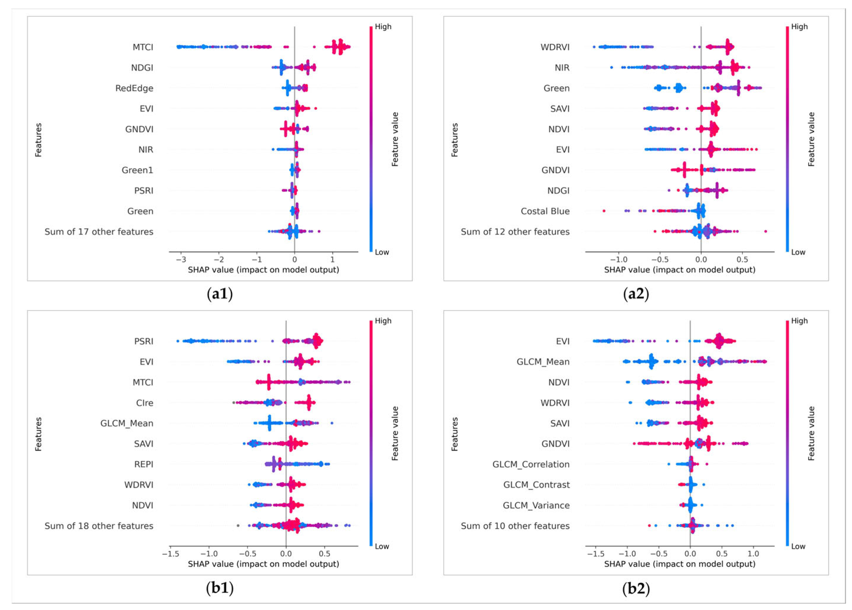
Figure 6 illustrates global SHAP results for PS and S2 red-edge schemes during the Heading–Flowering stage. Based on the overall ranking, red-edge-related indices consistently ranked among the top features in predictive contribution across both sensor conditions, indicating their strong association with rice variety identification.
In the PS scheme without red-edge features (Figure 6(a2)), WDRVI, NIR, and Green provided high predictive contributions. In the corresponding red-edge scheme (Figure 6(a1)), red-edge-related features show high contribution levels, with MTCI presenting the highest mean absolute SHAP value, suggesting its strong influence within the model. For the S2 scheme without red-edge features (Figure 6(b2)), EVI and mean texture features provided the highest predictive contributions, with their mean absolute SHAP values exceeding those of other features. In the red-edge scheme (Figure 6(b1)), PSRI, EVI, and MTCI exhibit the highest predictive contributions. Among the top three features ranked by predictive contribution, two are red-edge indices, and PSRI presents the foremost predictive contribution.
In contrast, in schemes excluding red-edge information, visible, NIR, and texture features exhibit relatively higher contributions. However, the overall magnitude of feature contributions is relatively lower, and the ranking structure is more dispersed. This pattern suggests that, in the absence of red-edge information, model predictions distribute across multiple spectral and texture features, which may explain the comparatively lower discriminative performance observed.

3.2.2. Feature Prediction Paths

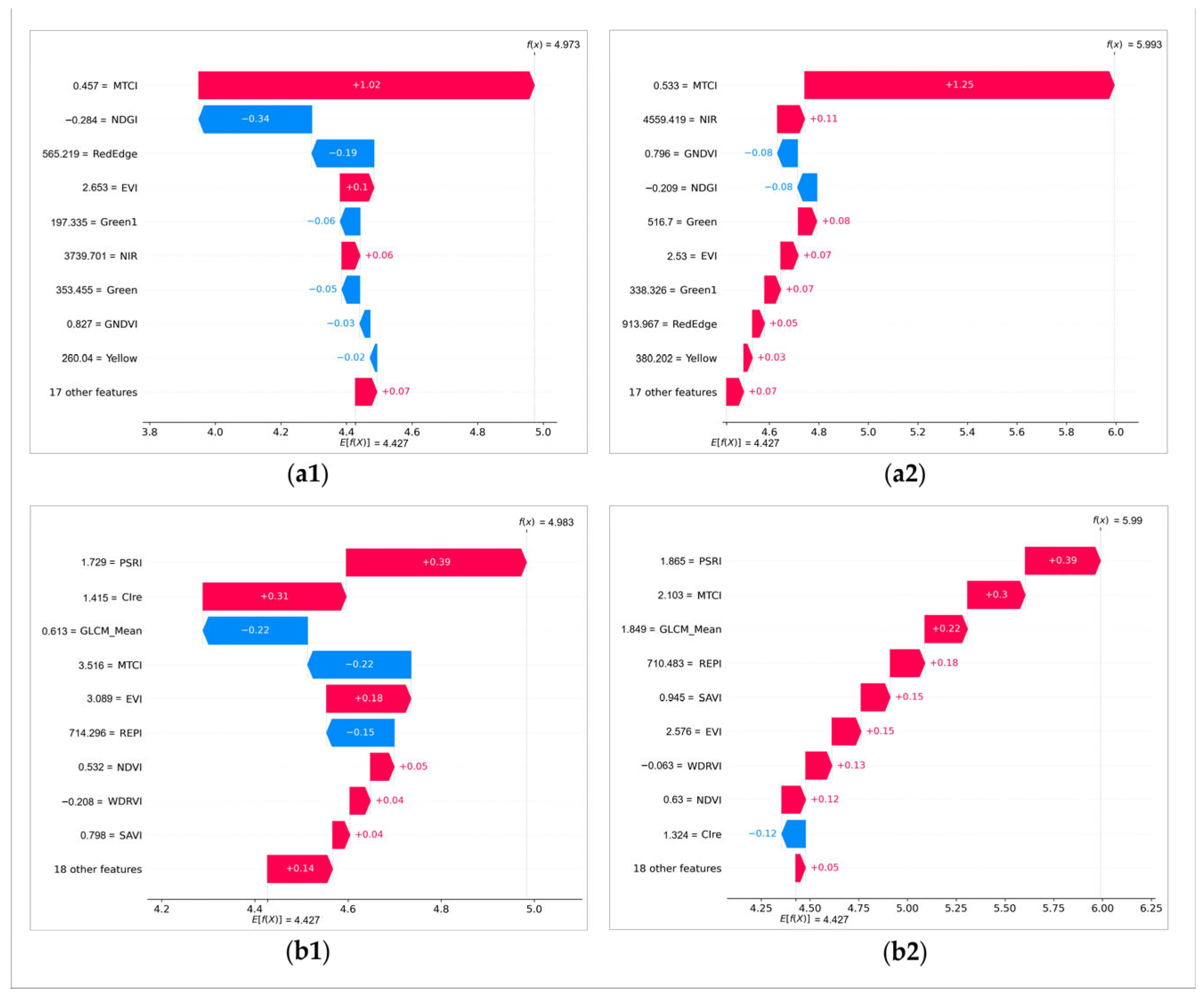
Building on global feature contribution analysis, we further select representative samples of Japonica and Indica rice for local SHAP analysis to explore prediction behavior at the individual sample level and reveal differences in decision paths among different models. The criterion for selecting representative samples is defined by the degree to which the sample predicted values approximate the average predicted value of the corresponding category. Specifically, samples with predicted values closest to the category-wise average are selected as representative samples for local SHAP analysis. Figure 7 illustrates local SHAP results.
Local SHAP analysis of the PS red-edge schemes (Figure 7(a1,a2)) shows that red-edge-related features, particularly MTCI, show strong positive contributions to the prediction probability for Japonica and Indica rice samples. Contribution patterns of typical samples for both varieties remain consistent, with individual red-edge features making major contribution, suggesting consistent contribution patterns across samples.
Local SHAP analysis of the S2 red-edge schemes (Figure 7(b1,b2)) demonstrates that multiple red-edge indices (such as PSRI, CLRE, and MTCI) simultaneously contribute to the prediction paths of Japonica and Indica rice. Although the degree of contribution varies among different indices, red-edge features collectively show the highest contribution levels in the model predictions. Local SHAP analysis indicates that red-edge features are among the most influential factors in sample-level discrimination of rice varieties for both sensors.

3.3. Comparison of Identification Performance Under Different Red-Edge Configurations

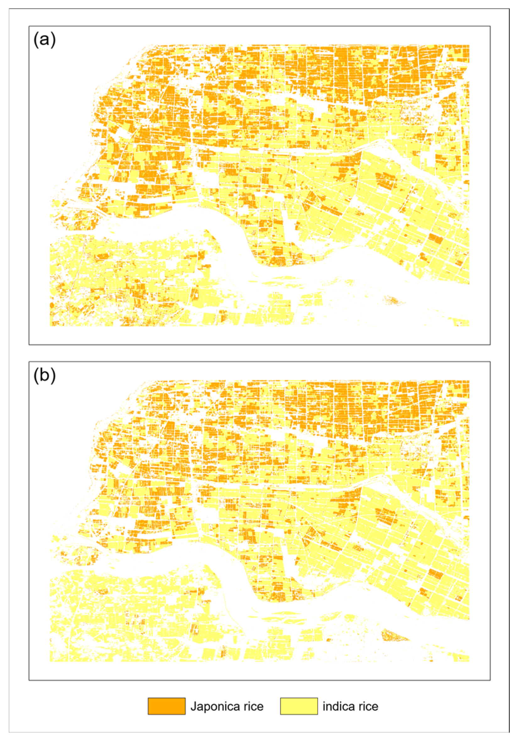
Based on the observed improvement associated with red-edge information for rice variety identification, we further compare classification performance under different red-edge configurations. Results indicate that although S2 imagery possesses multiple red-edge bands, its overall classification performance in rice variety identification is not substantially superior to the PS schemes that include only a single red-edge band. Specifically, at the Heading–Flowering stage, the F1-scores for Japonica and Indica rice obtained by the red-edge schemes of both sensors are similar. In Scheme 4, average F1-scores for Japonica and Indica rice are 98.24% and 98.49%, respectively, while in Scheme 8, they are 97.61% and 98.12%. We illustrate identification results for Scheme 4 and Scheme 8 in Figure 8; spatial structures of Japonica and Indica rice are similar across different results, both effectively representing the distribution of different rice varieties.
These results suggest that a single red-edge band, when coupled with appropriate feature construction, can achieve performance comparable to multi-band configurations, supporting classification requirements at the variety level. Given the consistency of results across different classifiers and feature combinations, this pattern remains generally consistent across classifiers and feature combinations in this study. This indicates that increasing the number of red-edge bands did not lead to proportional performance gains under the evaluated conditions, suggesting that multi-red-edge configurations may introduce partially overlapping spectral information for this specific task.

3.4. Comparison of Local Classification Results Under Different Spatial Resolutions

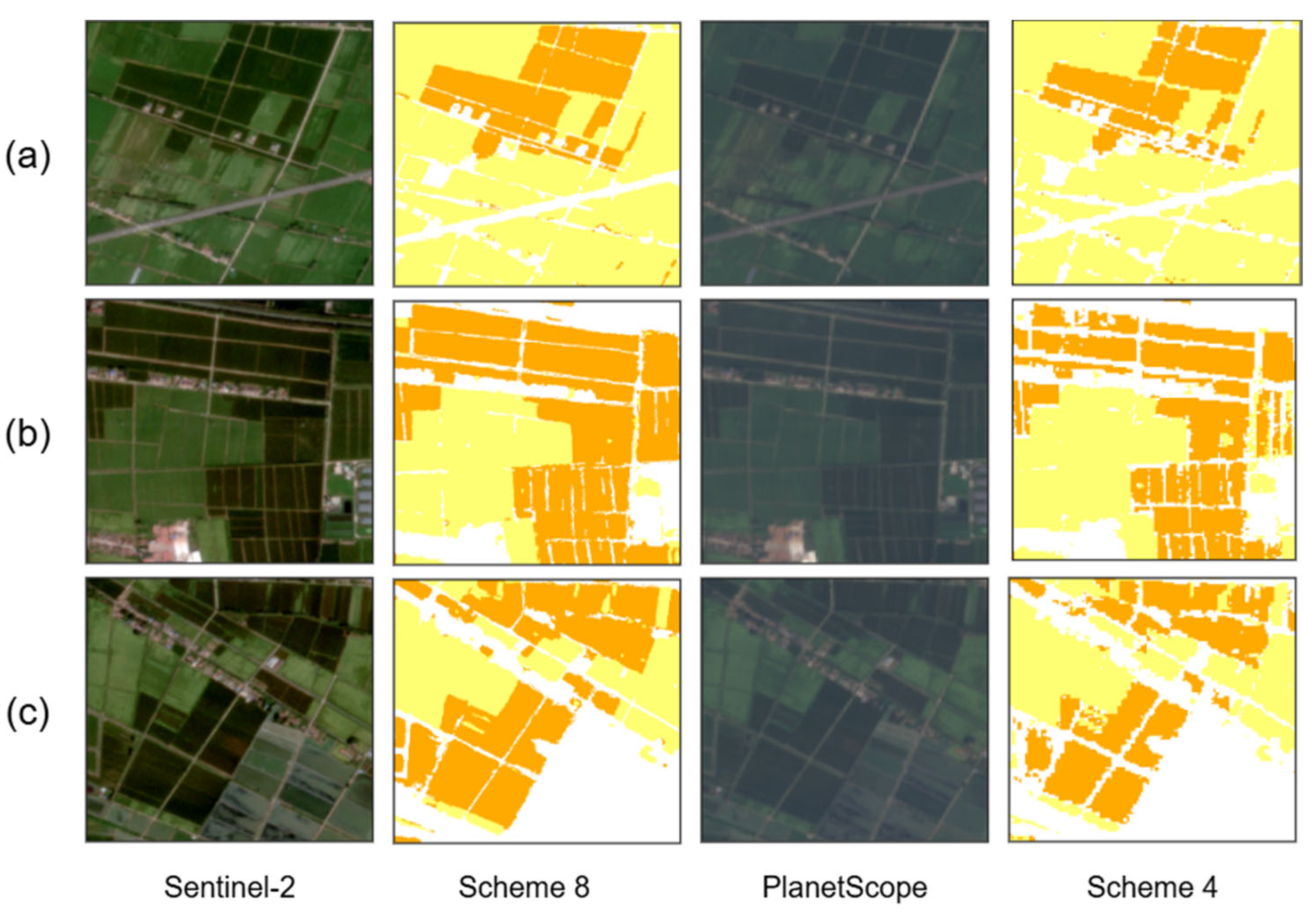
To visually demonstrate the spatial performance of rice variety identification under different sensor conditions, this study selects typical areas for local comparative analysis between PS and S2 classification results, as illustrated in Figure 9.
Results indicate that PS classification maps provide a clearer representation of field boundaries and small-scale planting structures, with classification results appearing more spatially continuous. In contrast, S2 classification results exhibit a certain degree of mixed pixel effect in some small plot areas, leading to relatively blurred classification boundaries. Regardless of the sensor used, red-edge schemes demonstrated more reasonable spatial distribution characteristics, reducing misclassification both within fields and along boundary areas.

3.5. Comparison with Previous Studies

To evaluate the reliability and scientific contribution of this research, we compare our results regarding classification accuracy, red-edge efficacy, and sensor performance with representative studies in the field (Table 6).
In terms of accuracy, discriminating intra-species cultivars is notably more challenging than identifying broad crop types. Islam et al. noted that cultivar discrimination rarely exceeds 95% due to high spectral similarity. By integrating red-edge information within an optimized scheme, our study achieved a 98.14% OA.
Regarding feature efficacy, our results support the findings of Kang et al. on red-edge gains but further reveal that increasing red-edge band counts does not yield proportional accuracy improvements. This aligns with the spectral redundancy theory proposed by Otunga et al., suggesting that for variety-level tasks, the sensitivity of red-edge information is more critical than band quantity. Furthermore, the comparison between PS and S2 echoes the views of Frazier and Hemingway and Andreatta et al.: in smaller size fields, PS’s superior 3-m spatial resolution provides clearer boundary delineation, successfully compensating for its lower spectral dimensionality.
Finally, the phenological sensitivity observed here is highly consistent with Rahmati et al. The heading–flowering stage exhibited the highest discriminative power across all experimental schemes due to the maximum divergence in canopy structure and physiological traits. This underscores that selecting the correct phenological window is a more fundamental prerequisite for high-accuracy cultivar mapping than sensor hardware specifications alone.

4. Discussion

4.1. Identification Advantages of the Heading–Flowering Stage

Analysis outcomes reveal that both PS and S2 imagery yield the highest accuracy in discriminating Indica and Japonica rice during the Heading–Flowering stage, whereas classification performance is evidently lower at the Tillering–Jointing stage. This consistent trend appears across all feature configuration schemes and classification algorithms, demonstrating that phenological stage acts as a core determinant of remote sensing-based rice variety identification performance. From the perspective of crop growth physiology, the Heading–Flowering stage marks a pivotal developmental transition for rice, where the crop shifts from vegetative growth to reproductive growth [43]. During this key phase, inherent differences in canopy architecture, leaf morphological traits, and physiological status between Indica and Japonica rice become significantly amplified, creating prominent and distinguishable spectral and spatial features that facilitate accurate remote sensing discrimination of the two rice varieties [44,45].
From the perspective of remote sensing observation, the rice canopy structure reaches a relatively stable state during the Heading–Flowering stage, which makes the intervarietal differences in Leaf Area Index (LAI) and leaf arrangement patterns highly detectable in the spectral and spatial features captured by remote sensing sensors [22]. In contrast, at the Tillering–Jointing stage, canopies of different rice varieties remain in the developmental stage and are not fully formed; meanwhile, the high level of internal spatial heterogeneity within rice fields leads to unstable and inconsistent spectral response characteristics between Indica and Japonica rice, which elevates uncertainty in remote sensing-based variety identification [46]. These findings further confirm that targeted selection of key phenological growth stages is a crucial and effective strategy to enhance the classification reliability of rice variety remote sensing mapping.

4.2. Mechanism of Red-Edge Information in Rice Variety Identification

Located in the spectral gap between the visible and near-infrared regions, the red-edge band exhibits ultra-high sensitivity to variations in vegetation chlorophyII content, nitrogen nutritional status, and canopy structural properties [47]. Across all experimental settings involving different sensors and phenological stages, this study consistently finds that integrating red-edge spectral information leads to a significant improvement in the accuracy of Indica and Japonica rice identification. Furthermore, both global and local SHAP interpretability analyses verify that red-edge-related features contribute most prominently to the model’s decision-making process, indicating that red-edge information holds stable and unique discriminative value for differentiating of rice varieties.
Comparative global SHAP analysis across different schemes reveals that for scenarios without red-edge bands, the models primarily rely on non-red-edge features and spatial texture features. After the introduction of red-edge information, the model dependence shifts toward red-edge-related indices such as PSRI and MTCI. This shift indicates that in the absence of red-edge bands the models have to rely on alternative features with relatively lower sensitivity.
There are inherent differences in vegetation physiological characteristics between Indica and Japonica rice, yet such differences cannot be effectively distinguished by less sensitive non-red-edge features. Consequently, these non-red-edge features generally yield low absolute SHAP values, accompanied by a flattened and scattered feature importance ranking. Such dispersed decision mechanisms force the model to integrate numerous weakly correlated features for classification inference, which not only reduces discriminative efficiency but also mechanistically explains the inferior overall classification accuracy of schemes without red-edge information.
Local SHAP analysis further demonstrates distinct feature utilization mechanisms in red-edge schemes of different sensors. For PS equipped with only a single red-edge band, the model presents a single-feature-driven prediction pattern, where highly correlated individual indicators dominate and determine the prediction probability of Indica and Japonica rice. This reflects that under the constraint of limited spectral dimensions, the model fully exploits the discriminative potential of the sole red-edge band and its derived vegetation indices. In contrast, the red-edge scheme of S2 adopts a multi-feature collaborative decision-making mode, in which multiple red-edge indices including PSRI, Clre and MTCI jointly contribute to sample classification and prediction.
In terms of physiological mechanisms, Indica and Japonica rice exhibit intrinsic differences in chlorophyII content, nitrogen uptake efficiency, and photosynthetic physiological characteristics, and these differences become increasingly pronounced during the middle and late stages of rice growth [48]. Such subtle yet essential physiological variations are often difficult to be fully capture and distinguish using traditional visible spectral bands alone [7]. In contrast, the red-edge band is highly sensitive to gradient changes in chlorophyII concentration in rice leaves, which endows it with an unparalleled advantage in the fine-grained discrimination of rice varieties. Additionally, red-edge vegetation indices can effectively mitigate interference from background soil reflectance and variable illumination conditions in the study area, which enhances the stability of vegetation signal expression in remote sensing imagery and strengthens the model’s ability to capture and respond to the inherent differences between rice varieties [49].
Notably, the discriminative effectiveness of red-edge information is not consistent across different rice phenological stages. This study finds that the improvement in rice variety identification accuracy brought by incorporating of red-edge features is significantly more pronounced at the Tillering–Jointing stage than at the Heading–Flowering stage. This phenomenon further illustrates that the practical utility of red-edge spectral information highly depends on precise matching between the physiological growth state of the crop and the timing of remote sensing observation. It also highlights that high-accuracy discrimination of rice varieties relies on the synergistic interaction between red-edge information and phenological stage selection, rather than standalone application of red-edge spectral features.

4.3. Insights into Sensor Red-Edge Configurations

A striking finding of this study is that PS imagery, equipped with a single red-edge band, achieves classification performance comparable to that of S2 imagery with its multi-red-edge band configuration in the task of rice variety identification. This result indicates that simply increasing the number of red-edge bands does not produce a linear or proportional improvement in the accuracy of variety-level crop remote sensing identification.
From the perspective of information utilization, multi red-edge bands may entail spectral information redundancy to a certain extent. The three red-edge bands of S2 are geographically adjacent in the spectral dimension, all located within the spectral range where vegetation reflectance rises sharply. Accordingly, a moderate linear correlation exists among these different red-edge bands [50]. In such cases, additional red-edge bands contribute very limitedly to improving of the model’s discriminative power. On the contrary, the superior high spatial resolution of PS imagery endows it with a distinctive advantage in delineating fine-scale field boundaries, complex rice planting structures, and detailed spatial texture characteristics of the study area, which effectively compensates for the limitation of having only a single red-edge band [51]. This demonstrates that the effectiveness of red-edge information in rice variety identification is not determined by the number of red-edge bands alone, but is jointly regulated by the complex interplay of spatial resolution, feature construction methods, and phenological stage selection.
This finding provides important practical insights for the selection and application of remote sensing sensors in agricultural monitoring: in complex and highly fragmented agricultural landscapes, a rational combination of high spatial resolution and key spectral information (e.g., a single red-edge band) is more conducive to improving the accuracy and reliability of crop variety mapping than merely pursuing an increase in spectral dimensionality by adding more red-edge bands. This discovery also offers valuable references for the design of future agricultural remote sensing satellite payloads and the development of remote sensing data application strategies, suggesting that on the premise of meeting the requirements of key spectral bands for agricultural monitoring, comprehensive and priority consideration should be given to the spatial resolution and observational frequency of satellite sensors during the design process.

4.4. Limitations and Potential for Promotion

Although this study systematically evaluates the impacts of different remote sensing sensors, red-edge band configurations, and phenological stages on rice variety identification, it still has certain inherent limitations that require addressing in subsequent research. First, the research is conducted based on remote sensing data and field survey samples from a single year and a single typical rice-growing region, and thus fails to fully account for the potential impacts of interannual climate variability (e.g., temperature, precipitation) and regional differences in agricultural management practices on the spectral characteristics of different rice varieties [52,53]. Second, different rice field management measures may lead to differences in the red-edge spectral responses of rice, yet this study does not separate and analyze the influence of such management factors independently [54].
Nevertheless, the analytical framework and core research conclusions proposed in this study exhibit strong applicability and promotion potential in the field of remote sensing-based rice variety mapping. By selecting key phenological growth stages of rice, fully exploiting the discriminative value of red-edge spectral information, and integrating the advantages of high spatial resolution remote sensing data, it is possible to achieve more reliable and accurate rice variety identification under existing multi-source remote sensing data conditions. This research can provide important technical support for the fine-scale monitoring of precision agriculture, dynamic assessment of regional rice variety planting structures, and scientific evaluation of food production capacity.

5. Conclusions

This study systematically evaluated the synergistic effects of spatial resolution, red-edge configuration, and phenological scheduling on rice cultivar identification. In response to the three research objectives proposed in the introduction, the main conclusions are summarized as follows:
First, regarding the overall capability of rice cultivar identification, both PS and S2 exhibited strong and highly accurate classification performance. The red-edge feature schemes and baseline feature schemes of the two sensors both achieved high overall accuracy (all above 97%), demonstrating their great potential in finely distinguishing Indica and Japonica rice.
Second, findings concerning the impacts of phenological stages and red-edge information indicated that the Heading and Flowering stage constitutes a critical period for cultivar differentiation, achieving higher identification accuracy than other periods for both sensors. Furthermore, the incorporation of red-edge features significantly enhanced the discriminative ability across all experimental schemes. Global and local SHAP analyses further confirmed that red-edge indices play a dominant role in the model decision-making process.
Third, the investigation into the efficiency differences of red-edge configurations revealed that merely increasing the number of red-edge bands may introduce spectral redundancy and does not guarantee a substantial improvement in cultivar identification performance. The PS schemes with only one red-edge band still achieved comparable classification performance to the multi red-edge schemes of S2, highlighting the importance of the synergistic interaction among high spatial resolution, red-edge information, and phenology.
For fragmented agricultural regions or small-scale farms, the use of PS for cultivar-level crop mapping enables high-precision identification at the plot scale. For large-scale and continuous mapping tasks, S2 provides a highly cost-effective alternative. Although this study validates the effectiveness of the proposed schemes, it is limited by data acquired from a single year and a specific region and insufficiently considers field-level management differences. Future research will focus on multi-year validation across broader agricultural regions and the integration of optical, SAR, and LiDAR data to more reliably map crop cultivar distributions under complex environmental conditions.

Author Contributions

Conceptualization, Y.W. and Y.Z.; methodology, K.S., Y.L. and H.M.; software, Y.X. and Y.C.; validation, Z.X. and L.H.; formal analysis, Y.W., Y.Z. and K.S.; investigation, Y.L. and H.M.; resources, Y.W., K.S. and Z.X.; writing—original draft preparation, Y.W. and Y.Z.; writing—review and editing, Y.L., Y.C. and L.H.; funding acquisition, Y.W., Y.Z. and Z.X. All authors have read and agreed to the published version of the manuscript.

Funding

This research was funded by 2024 Jiangsu Province Natural Resources Science and Technology Innovation Project (Research on the Construction of Jiangsu Province Natural Resources Satellite Application System), grant number JSZRKJ202417; Research on the Construction of Dynamic Monitoring Network for Natural Resources in Xinyi City, Jiangsu Province in 2024, grant number 2024007; Demonstration of Meteorological Risk Warning, Prevention, and Disaster Reduction Technologies for Grain and Oil Production in Jiangsu Province under Climate Change, grant number CTG[2025]01-5-2; the national key research and development project “fine monitoring and early warning and prevention and control measures for key areas of green tide of Enteromorpha prolifera in the Yellow Sea” Project 3 “Research on key technologies for early fine monitoring of green tide of Enteromorpha prolifera in the Yellow Sea”, grant number 2024YFC3109003; Natural Resources Research Projects of Jiangsu Province Project Name: Research on the Construction of Natural Resources Dynamic Monitoring Network in Xinyi City, grant number 2024007.

Institutional Review Board Statement

Not applicable.

Informed Consent Statement

Not applicable.

Data Availability Statement

Data are available under request from the authors.

Acknowledgments

The authors would like to express gratitude for the PlanetScope images provided by Planet Satellite Company and the Sentinel-2 images provided by the European Space Agency.

Conflicts of Interest

The authors declare that this study received support from Planet Satellite Company in the form of satellite imagery. The funder was not involved in the study design, collection, analysis, interpretation of data, the writing of this article, or the decision to submit it for publication.

References

  1. Fang, H.; Liang, S.; Chen, Y.; Ma, H.; Li, W.; He, T.; Tian, F.; Zhang, F. A comprehensive review of rice mapping from satellite data: Algorithms, product characteristics and consistency assessment. Sci. Remote Sens. 2024, 10, 100172. [Google Scholar] [CrossRef] [Scilit]
  2. Yuan, S.; Linquist, B.A.; Wilson, L.T.; Cassman, K.G.; Stuart, A.M.; Pede, V.; Miro, B.; Saito, K.; Agustiani, N.; Aristya, V.E.; et al. Sustainable intensification for a larger global rice bowl. Nat. Commun. 2021, 12, 7163. [Google Scholar] [CrossRef] [Scilit]
  3. Zhao, L.; Luo, Z.; Zhou, K.; Yang, B.; Zhang, Y. Fine classification of rice fields in high-resolution remote sensing images. Sci. Rep. 2024, 14, 20778. [Google Scholar] [CrossRef] [Scilit] [PubMed]
  4. Islam, M.M.; Himel, G.M.S.; Moazzam, M.G.; Uddin, M.S. Artificial intelligence-based rice variety classification: A state-of-the-art review and future directions. Smart Agric. Technol. 2025, 10, 100788. [Google Scholar] [CrossRef] [Scilit]
  5. Becker-Reshef, I.; Barker, B.; Whitcraft, A.; Oliva, P.; Mobley, K.; Justice, C.; Sahajpal, R. Crop type maps for operational global agricultural monitoring. Sci. Data 2023, 10, 172. [Google Scholar] [CrossRef] [Scilit] [PubMed]
  6. Zhou, Y.N.; Zhu, W.W.; Feng, L.; Gao, J.W.; Chen, Y.H.; Zhang, X.; Luo, J.C. Hierarchical classification for improving parcel-scale crop mapping using time-series Sentinel-1 data. J. Environ. Manag. 2024, 369, 122251. [Google Scholar] [CrossRef] [Scilit]
  7. Kang, Y.; Meng, Q.; Liu, M.; Zou, Y.; Wang, X. Crop classification based on red edge features analysis of GF-6 WFV data. Sensors 2021, 21, 4328. [Google Scholar] [CrossRef] [Scilit]
  8. Tufail, R.; Tassinari, P.; Torreggiani, D. Deep learning applications for crop mapping using Multi-Temporal sentinel-2 data and Red-Edge vegetation indices: Integrating convolutional and recurrent neural networks. Remote Sens. 2025, 17, 3207. [Google Scholar] [CrossRef] [Scilit]
  9. Xie, Y.; Zeng, H.; Li, J.; Zhao, H.; Yu, Q.; Qiu, B.; Ahmed, S.; Wu, B. Improving parcel level crop classification by integrating a novel red edge maize-cotton mapping index and machine learning: A case study in the Ebinur Lake Basin. Int. J. Appl. Earth Obs. Geoinf. 2025, 143, 104765. [Google Scholar] [CrossRef] [Scilit]
  10. Dong, T.; Liu, J.; Shang, J.; Qian, B.; Ma, B.; Kovacs, J.M.; Walters, D.; Jiao, X.; Geng, X.; Shi, Y. Assessment of red-edge vegetation indices for crop leaf area index estimation. Remote Sens. Environ. 2019, 222, 133–143. [Google Scholar] [CrossRef] [Scilit]
  11. Li, D.; Cheng, T.; Zhou, K.; Zheng, H.; Yao, X.; Tian, Y.; Zhu, Y.; Cao, W. WREP: A wavelet-based technique for extracting the red edge position from reflectance spectra for estimating leaf and canopy chlorophyll contents of cereal crops. ISPRS J. Photogramm. Remote Sens. 2017, 129, 103–117. [Google Scholar] [CrossRef] [Scilit]
  12. Otunga, C.; Odindi, J.; Mutanga, O.; Adjorlolo, C. Evaluating the potential of the red edge channel for C3 (Festuca spp.) grass discrimination using Sentinel-2 and Rapid Eye satellite image data. Geocarto Int. 2019, 34, 1123–1143. [Google Scholar] [CrossRef] [Scilit]
  13. Zeng, L.; Wardlow, B.D.; Xiang, D.; Hu, S.; Li, D. A review of vegetation phenological metrics extraction using time-series, multispectral satellite data. Remote Sens. Environ. 2020, 237, 111511. [Google Scholar] [CrossRef] [Scilit]
  14. Gara, T.W.; Darvishzadeh, R.; Skidmore, A.K.; Wang, T. Impact of Vertical Canopy Position on Leaf Spectral Properties and Traits across Multiple Species. Remote Sens. 2018, 10, 346. [Google Scholar] [CrossRef] [Scilit]
  15. Rahmati, A.; Zoej, M.J.V.; Dehkordi, A.T. Early identification of crop types using Sentinel-2 satellite images and an incremental multi-feature ensemble method (Case study: Shahriar, Iran). Adv. Space Res. 2022, 70, 907–922. [Google Scholar] [CrossRef] [Scilit]
  16. Tran, K.H.; Zhang, X.; Ketchpaw, A.R.; Wang, J.; Ye, Y.; Shen, Y. A novel algorithm for the generation of gap-free time series by fusing harmonized Landsat 8 and Sentinel-2 observations with PhenoCam time series for detecting land surface phenology. Remote Sens. Environ. 2022, 282, 113275. [Google Scholar] [CrossRef] [Scilit]
  17. Ouzemou, J.; Harti, A.E.; Lhissou, R.; Moujahid, A.E.; Bouch, N.; Ouazzani, R.E.; Bachaoui, E.M.; Ghmari, A.E. Crop type mapping from pansharpened Landsat 8 NDVI data: A case of a highly fragmented and intensive agricultural system. Remote Sens. Appl. Soc. Environ. 2018, 11, 94–103. [Google Scholar] [CrossRef] [Scilit]
  18. Frazier, A.E.; Hemingway, B.L. A technical review of planet smallsat data: Practical considerations for processing and using PlanetScope imagery. Remote Sens. 2021, 13, 3930. [Google Scholar] [CrossRef] [Scilit]
  19. Drusch, M.; Bello, U.D.; Carlier, S.; Colin, O.; Fernandez, V.; Gascon, F.; Hoersch, B.; Isola, C.; Laberinti, P.; Martimort, P.; et al. Sentinel-2: ESA’s optical High-Resolution mission for GMES operational services. Remote Sens. Environ. 2012, 120, 25–36. [Google Scholar] [CrossRef] [Scilit]
  20. Zhen, Z.; Quackenbush, L.J.; Stehman, S.V.; Zhang, L. Impact of training and validation sample selection on classification accuracy and accuracy assessment when using reference polygons in object-based classification. Int. J. Remote Sens. 2013, 34, 6914–6930. [Google Scholar] [CrossRef] [Scilit]
  21. Karasiak, N.; Dejoux, J.F.; Monteil, C.; Sheeren, D. Spatial dependence between training and test sets: Another pitfall of classification accuracy assessment in remote sensing. Mach. Learn. 2022, 111, 2715–2740. [Google Scholar] [CrossRef] [Scilit]
  22. Li, C.; Teng, X.; Tan, Y.; Zhang, Y.; Zhang, H.; Xiao, D.; Luo, S. Spatio-temporal mapping of leaf area index in rice: Spectral indices and multi-scale texture comparison derived from different sensors. Front. Plant Sci. 2024, 15. [Google Scholar] [CrossRef] [Scilit]
  23. Boiarskii, B. Comparison of NDVI and NDRE indices to detect differences in vegetation and chlorophyll content. J. Mech. Contin. Math. Sci. 2019, 4, 20–29. [Google Scholar] [CrossRef] [Scilit]
  24. Dash, J.; Curran, P.J. Evaluation of the MERIS terrestrial chlorophyll index (MTCI). Adv. Space Res. 2007, 39, 100–104. [Google Scholar] [CrossRef] [Scilit]
  25. Matsushita, B.; Yang, W.; Chen, J.; Onda, Y.; Qiu, G. Sensitivity of the enhanced vegetation index (EVI) and normalized difference vegetation index (NDVI) to topographic effects: A case study in high-density cypress forest. Sensors 2007, 7, 2636–2651. [Google Scholar] [CrossRef] [Scilit]
  26. Haralick, R.M.; Shanmugam, K.; Dinstein, I. Textural features for image classification. Stud. Media Commun. 1973, SMC-3, 610–621. [Google Scholar] [CrossRef] [Scilit]
  27. Kanan, C.; Cottrell, G.W. Color-to-grayscale: Does the method matter in image recognition? PLoS ONE 2012, 7, e29740. [Google Scholar] [CrossRef] [Scilit]
  28. Khatami, R.; Mountrakis, G.; Stehman, S.V. A meta-analysis of remote sensing research on supervised pixel-based land-cover image classification processes: General guidelines for practitioners and future research. Remote Sens. Environ. 2016, 177, 89–100. [Google Scholar] [CrossRef] [Scilit]
  29. García, M.A.; Puig, D. Supervised texture classification by integration of multiple texture methods and evaluation windows. Image Vis. Comput. 2007, 25, 1091–1106. [Google Scholar] [CrossRef] [Scilit]
  30. Hall-Beyer, M. Practical guidelines for choosing GLCM textures to use in landscape classification tasks over a range of moderate spatial scales. Int. J. Remote Sens. 2017, 38, 1312–1338. [Google Scholar] [CrossRef] [Scilit]
  31. Mohammadpour, P.; Viegas, D.X.; Viegas, C. Vegetation mapping with random forest using sentinel 2 and GLCM texture feature—A case study for lousã region, portugal. Remote Sens. 2022, 14, 4585. [Google Scholar] [CrossRef] [Scilit]
  32. Montero, D.; Aybar, C.; Mahecha, M.D.; Martinuzzi, F.; Söchting, M.; Wieneke, S. A standardized catalogue of spectral indices to advance the use of remote sensing in Earth system research. Sci. Data 2023, 10, 197. [Google Scholar] [CrossRef] [Scilit] [PubMed]
  33. Andreatta, D.; Gianelle, D.; Scotton, M.; Dalponte, M. Estimating grassland vegetation cover with remote sensing: A comparison between Landsat-8, Sentinel-2 and PlanetScope imagery. Ecol. Indic. 2022, 141, 109102. [Google Scholar] [CrossRef] [Scilit]
  34. Wei, Y.; Lu, M.; Yu, Q.; Li, W.; Wang, C.; Tang, H.; Wu, W. The normalized difference yellow vegetation index (NDYVI): A new index for crop identification by using GaoFen-6 WFV data. Comput. Electron. Agric. 2024, 226, 109417. [Google Scholar] [CrossRef] [Scilit]
  35. Gitelson, A.A.; Viña, A.; Ciganda, V.; Rundquist, D.C.; Arkebauer, T.J. Remote estimation of canopy chlorophyll content in crops. Geophys. Res. Lett. 2005, 32, L8403. [Google Scholar] [CrossRef] [Scilit]
  36. Arik, S.Ö.; Pfister, T. TabNet: Attentive interpretable tabular learning. Proc. AAAI Conf. Artif. Intell. 2021, 35, 6679–6687. [Google Scholar] [CrossRef] [Scilit]
  37. Rodriguez-Galiano, V.F.; Ghimire, B.; Rogan, J.; Chica-Olmo, M.; Rigol-Sanchez, J.P. An assessment of the effectiveness of a random forest classifier for land-cover classification. ISPRS J. Photogramm. Remote Sens. 2012, 67, 93–104. [Google Scholar] [CrossRef] [Scilit]
  38. Ke, G.; Meng, Q.; Finley, T.; Wang, T.; Chen, W.; Ma, W.; Ye, Q.; Liu, T. LightGBM: A Highly Efficient Gradient Boosting Decision Tree. In Proceedings of the NIPS’17: Proceedings of the 31st International Conference on Neural Information Processing Systems, Long Beach, CA, USA, 4–9 December 2017; pp. 3149–3157. [Google Scholar]
  39. Akiba, T.; Sano, S.; Yanase, T.; Ohta, T.; Koyama, M. Optuna: A next-generation hyperparameter optimization framework. In Proceedings of the KDD’19: The 25th ACM SIGKDD Conference on Knowledge Discovery and Data Mining, Anchorage, AK, USA, 4–8 August 2019; pp. 2623–2631. [Google Scholar]
  40. Lundberg, S.M.; Lee, S. A unified approach to interpreting model predictions. In Proceedings of the NIPS’17: Proceedings of the 31st International Conference on Neural Information Processing Systems, Long Beach, CA, USA, 4–9 December 2017; pp. 4768–4777. [Google Scholar]
  41. Chen, H.; Lundberg, S.M.; Lee, S. Explaining a series of models by propagating Shapley values. Nat. Commun. 2022, 13, 4512. [Google Scholar] [CrossRef] [Scilit]
  42. Ghalebikesabi, S.; Ter-Minassian, L.; Diazordaz, K.; Holmes, C.C. On locality of local explanation models. In NIPS ‘21; Curran Associates, Inc.: Red Hook, NY, USA, 2021; p. 13. [Google Scholar]
  43. Yoshida, A.; Ohmori, Y.; Kitano, H.; Taguchi-Shiobara, F.; Hirano, H. Aberrant spikelet and panicle1, encoding a TOPLESS-related transcriptional co-repressor, is involved in the regulation of meristem fate in rice. Plant J. 2012, 70, 327–339. [Google Scholar] [CrossRef] [Scilit]
  44. Zhang, H.; Wang, L.; Jin, X.; Bian, L.; Ge, Y. High-throughput phenotyping of plant leaf morphological, physiological, and biochemical traits on multiple scales using optical sensing. Crop J. 2023, 11, 1303–1318. [Google Scholar] [CrossRef] [Scilit]
  45. Yin, M.; Liu, S.; Zheng, X.; Chu, G.; Xu, C.; Zhang, X.; Wang, D.; Chen, S. Solar radiation-use characteristics of indica/japonica hybrid rice (Oryza sativa L.) in the late season in southeast China. Crop J. 2021, 9, 427–439. [Google Scholar] [CrossRef] [Scilit]
  46. Manohar Kumar, C.V.S.S.; Jha, S.S.; Nidamanuri, R.R.; Dadhwal, V.K. Precision crop mapping: Within plant canopy discrimination of crop and soil using multi-sensor hyperspectral imagery. Sci. Rep. 2024, 14, 24903. [Google Scholar] [CrossRef] [Scilit] [PubMed]
  47. Hallik, L.; Kuusk, A.; Lang, M.; Kuusk, J. Reflectance properties of hemiboreal mixed forest canopies with focus on red edge and near infrared spectral regions. Remote Sens. 2019, 11, 1717. [Google Scholar] [CrossRef] [Scilit]
  48. Zhou, N.; Sun, T.; Zhang, Y.; Shi, Q.; Zhou, Y.; Xiong, Q.; Hu, J.; Wang, S.; Zhu, J. Comparative analysis of yield and Grain-Filling characteristics of conventional rice with different panicle types in response to nitrogen fertilization. Agronomy 2025, 15, 1858. [Google Scholar] [CrossRef] [Scilit]
  49. Pinheiro, H.S.K.; Barbosa, T.P.R.; Antunes, M.A.H.; Carvalho, D.C.D.; Nummer, A.R.; Carvalho Junior, W.D.; Chagas, C.D.S.; Fernandes-Filho, E.I.; Pereira, M.G. Assessment of phytoecological variability by Red-Edge spectral indices and Soil-Landscape relationships. Remote Sens. 2019, 11, 2448. [Google Scholar] [CrossRef] [Scilit]
  50. Wang, B.; Jia, K.; Liang, S.; Xie, X.; We, X.; Zhao, X.; Yao, Y.; Zhang, X. Assessment of Sentinel-2 MSI Spectral Band Reflectances for Estimating Fractional Vegetation Cover. Remote Sens. 2018, 10, 1927. [Google Scholar] [CrossRef] [Scilit]
  51. Chen, K. High-resolution winter cover crop mapping with PlanetScope imagery: Comparative analysis of Random Forest, Convolutional Neural Network, and unsupervised classification. Sci. Remote Sens. 2026, 13, 100351. [Google Scholar] [CrossRef] [Scilit]
  52. Gurgel, H.C.; Author, N.J.F.C. Annual and interannual variability of NDVI in Brazil and its connections with climate. Int. J. Remote Sens. 2003, 24, 3595–3609. [Google Scholar] [CrossRef] [Scilit]
  53. Garcia, M.; Ustin, S.L. Detection of interannual vegetation responses to climatic variability using AVIRIS data in a coastal savanna in California. IEEE Trans. Geosci. Remote Sens. 2001, 39, 1480–1490. [Google Scholar] [CrossRef]
  54. Mutanga, O.; Skidmore, A.K. Red edge shift and biochemical content in grass canopies. ISPRS J. Photogramm. Remote Sens. 2007, 62, 34–42. [Google Scholar] [CrossRef] [Scilit]
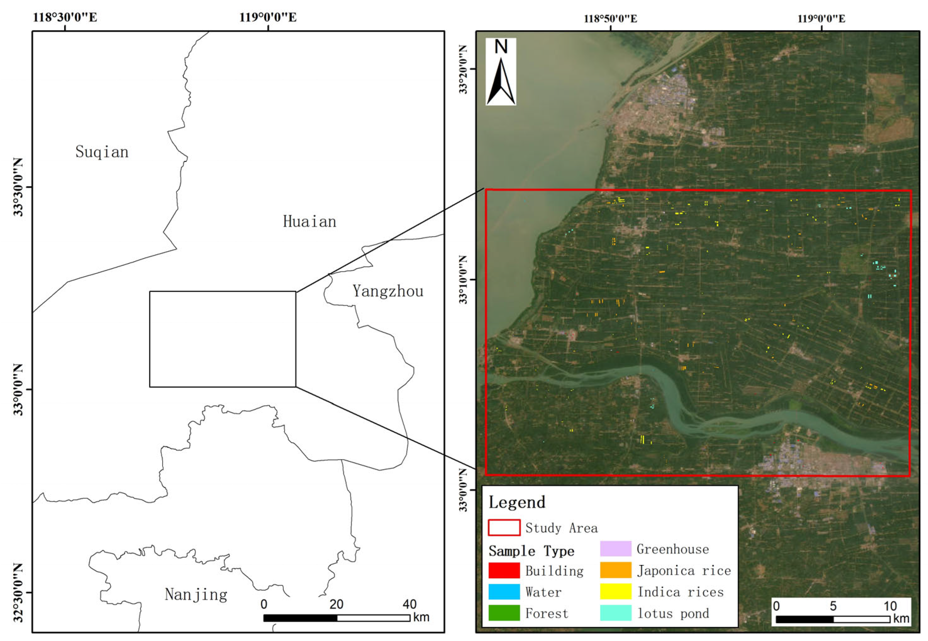
Figure 1. Geographical location of the study area and sample distribution.
Agriengineering 08 00187 g001
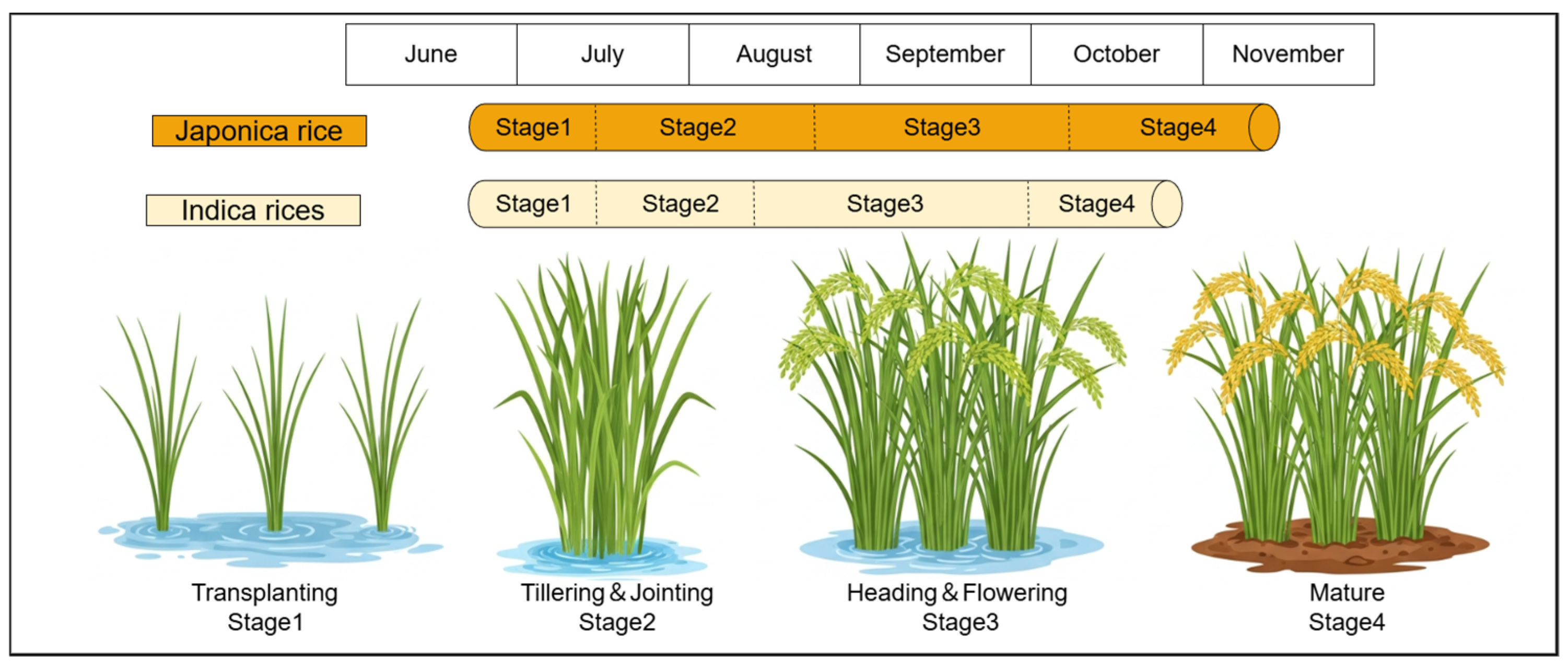
Figure 2. Rice phenological stages in the study area.
Agriengineering 08 00187 g002
Figure 3. Overview of the proposed workflow for evaluating red-edge band configuration for rice variety mapping.
Agriengineering 08 00187 g003
Figure 4. Comparison of classification accuracies across different classifiers.
Agriengineering 08 00187 g004
Figure 5. Spectral reflectance of Japonica and Indica rice at different phenological stages: (a1) reflectance of Japonica and Indica rice from PS data at the Tillering–Jointing stage; (a2) PS data at the Heading–Flowering stage; (b1) S2 data at the Tillering–Jointing stage; (b2) S2 data at the Heading–Flowering stage. The error bars represent the range of ±1 standard deviation. Bands marked with an asterisk (*) indicate significant differences between Japonica and Indica rice based on the two-tailed t-test, with a significance level of p < 0.05.
Agriengineering 08 00187 g005
Figure 6. Results of global SHAP analysis: (a1) SHAP summary plot for Scheme 8; (a2) SHAP summary plot for Scheme 7; (b1) SHAP summary plot for Scheme 4; (b2) SHAP summary plot for Scheme 3. The SHAP values correspond to the raw outputs of global SHAP analysis.
Agriengineering 08 00187 g006
Figure 7. Results of local SHAP analysis: (a1,a2) are the SHAP waterfall plots for Japonica and Indica rice in Scheme 8; (b1,b2) are the SHAP waterfall plots for Japonica and Indica rice in Scheme 4; E(f(x)), the base value, is defined as the expected output of the model over the background dataset, representing the reference prediction in the absence of feature information; f(x) is the final predicted value for the sample after accounting for all feature contributions.
Agriengineering 08 00187 g007
Figure 8. Identification results of Japonica and Indica rice: (a) RF identification results for Scheme 8; (b) RF identification results for Scheme 4.
Agriengineering 08 00187 g008
Figure 9. Spatial details of Japonica and Indica rice identification results: (a) Area 1; (b) Area 2; (c) Area 3; Identification results for Scheme 8 and Scheme 4 were obtained using the RF model.
Agriengineering 08 00187 g009
Table 1. Spectral bands and spatial resolution parameters of PS and S2.
Data TypeSpectral BandSpatial Resolution
PlanetScopeBand1: Coastal Blue (431–452 nm)3 m
Band2: Blue (465–515 nm)
Band3: Green1 (513–549 nm)
Band4: Green (547–583 nm)
Band5: Yellow (600–620 nm)
Band6: Red (650–680 nm)
Band7: Red-Edge (697–713 nm)
Band8: Near infrared (NIR) (845–885 nm)
Sentinel-2Band1: Coastal Blue (433–453 nm)60 m
Band2: Blue (458–523 nm)10 m
Band3: Green (543–578 nm)
Band4: Red (650–680 nm)
Band5: Red-Edge1 (698–713 nm)20 m
Band6: Red-Edge2 (733–748 nm)
Band7: Red-Edge3 (773–793 nm)
Band8: Near infrared (NIR) (785–900 nm)10 m
Band9: Near infrared narrow (NIRn) (855–875 nm)20 m
Band10: Water vapor (935–955 nm)60 m
Band11: Shortwave infrared1(SWIR1) (1565–1655 nm)20 m
Band12: Shortwave infrared2(SWIR2) (2100–2280 nm)
Table 3. Detailed descriptions of different feature combination schemes.
Scheme TypeSensorPhenological StageBaseline FeaturesRed-Edge FeaturesDesign Objective
Scheme 1Sentinel-2Tillering–Jointing×Baseline (S2-T1)
Scheme 2Tillering–JointingRE impact in S2-T1
Scheme 3Heading–Flowering×Baseline (S2-T2)
Scheme 4Heading–FloweringRE impact in S2-T2
Scheme 5PlanetScopeTillering–Jointing×Baseline (PS-T1)
Scheme 6Tillering–JointingRE impact in PS-T1
Scheme 7Heading–Flowering×Baseline (PS-T2)
Scheme 8Heading–FloweringRE impact in PS-T2
Note: Baseline features consist of spectral bands (excluding red-edge), vegetation indices, and texture features. Red-edge features comprise red-edge spectral bands and red-edge vegetation indices. T1: Tillering–Jointing stage; T2: Heading–Flowering stage.
Table 4. Classification accuracy comparison of different feature combination schemes.
Scheme TypeClassification Model
RFLightGBMTabNet
OA (%)/Kappa CoefficientJaponica F1-Scores (%)/
Indica F1-Scores (%)
OA (%)/Kappa CoefficientJaponica F1-Scores (%)/
Indica F1-Scores (%)
OA (%)/Kappa CoefficientJaponica F1-Scores (%)/
Indica F1-Scores (%)
Scheme 191.77/0.882090.23/91.33 92.08/0.886990.73/91.84 91.44/0.8771 90.33/91.86
Scheme 294.21/0.917193.35/94.28 95.00/0.928594.36/94.91 94.20/0.9173 94.31/94.87
Scheme 396.16/0.9452 96.86/97.21 96.79/0.954197.31/97.73 96.36/0.9479 97.17/97.53
Scheme 497.87/0.9696 98.62/98.68 97.74/0.967798.31/98.60 97.45/0.9636 97.79/98.18
Scheme 591.52/0.8795 88.90/91.20 91.34/0.876688.92/90.62 91.21/0.8747 89.01/90.99
Scheme 694.30/0.9188 92.70/94.17 93.56/0.908391.64/93.06 93.43/0.9063 92.12/93.68
Scheme 796.56/0.9509 95.44/95.85 95.93/0.941994.73/95.10 96.32/0.9475 95.46/95.81
Scheme 898.14/0.9735 97.67/98.41 98.03/0.971997.44/98.11 97.93/0.9705 97.72/97.85
Table 5. Schemes selected for SHAP interpretability analysis.
Scheme IDSensorPhenological StageRed-Edge Configuration
Scheme 3Sentinel-2Heading–Flowering×
Scheme 4
Scheme 7PlanetScope×
Scheme 8
Table 6. Quantitative and qualitative comparison between the current study and existing literature.
Comparison DimensionRepresentative StudiesPrevious Research Key ConclusionsThe Results of This Study DemonstrateContribution
Red-Edge EfficacyKang et al. [7],
Otunga et al. [12]
Red-edge bands are highly sensitive to vegetation physiology, significantly improving crop classification accuracy.The introduction of red-edge features increased the F1-score around 1–4% across all schemes.Confirmed the robust and stable accuracy gains of red-edge information specifically in intra-species cultivar discrimination.
Variety Discrimination AccuracyIslam et al. [4]Cultivar-level discrimination is highly challenging; conventional accuracies typically plateau between 90% and 95%.The optimal scheme achieved an overall accuracy of 98.14%.Broke through existing accuracy bottlenecks for rice variety mapping by synergizing optimal phenology and spectral features.
Sensor Comparison (PS vs. S2)Frazier & Hemingway [18],
Andreatta et al. [32]
PS possesses a strong spatial advantage in fragmented landscapes, whereas S2 offers richer spectral dimensions.PS’s single red-edge scheme performed comparably to S2’s multi-red-edge scheme, with superior boundary delineation.Revealed that high spatial resolution can effectively compensate for lower spectral dimensionality, indicating potential spectral redundancy in multi-red-edge configurations.
Phenological SensitivityRahmati et al. [15]Crop identification accuracy is significantly higher in mid-to-late growth stages compared to early stages.Accuracies at the heading–flowering stage were consistently higher than at the tillering–jointing stage across all sensors.Established the heading–flowering stage as the optimal window for Indica and Japonica rice discrimination.
Disclaimer/Publisher’s Note: The statements, opinions and data contained in all publications are solely those of the individual author(s) and contributor(s) and not of MDPI and/or the editor(s). MDPI and/or the editor(s) disclaim responsibility for any injury to people or property resulting from any ideas, methods, instructions or products referred to in the content.