Article

Multimodal Sensing to Estimate Soil Organic Carbon Using Limited Samples from Paddy Fields

by
Nelundeniyage Sumuduni L. Senevirathne
1,
Parwit Chutichaimaytar
1 and
Tofael Ahamed
2,*
1
Graduate School of Science and Technology, University of Tsukuba, 1-1-1 Tennodai, Tsukuba 305-8577, Japan
2
Institute of Life and Environmental Sciences, University of Tsukuba, 1-1-1 Tennodai, Tsukuba 305-8577, Japan
*
Author to whom correspondence should be addressed.
AgriEngineering 2026, 8(5), 185; https://doi.org/10.3390/agriengineering8050185
Submission received: 11 March 2026 / Revised: 2 May 2026 / Accepted: 6 May 2026 / Published: 8 May 2026

Abstract

The analysis of soil carbon helps various sectors, including agriculture, in the context of monitoring soil health. In precision agriculture, decisions are made on the basis of site-specific information and thus have the potential to increase crop productivity more than is possible with traditional high-input agriculture. Site-specific information-based nutrition management, pest and disease management, and water management are the main areas of interest in the era of precision agriculture. Soil organic carbon (SOC) is one of the main components of the carbon cycle and impacts soil physical and chemical properties. Soil color is considered an indicator of soil carbon. In relation to soil physical properties, soil color has been used to determine SOC level and classification throughout history in a qualitative manner, and recently, researchers have shown interest in relating soil color data to quantify soil chemical properties. From spectroscopy-based color analysis to image-based color analysis, research has shown strong relationships between SOC and color properties. Therefore, with the improvement of technology to create smaller and portable sensors, the potential exists to automate the processes of soil chemical analysis to use them in precision agriculture. Two of the major limitations of these methodologies in research are the number of known soil samples required to calibrate a model (the majority of the models require more than 100 samples) and the use of expensive spectrometers with complex processes. Thus, the potential of individual farmers to deploy these methods is limited. This research was conducted to develop a methodology with complete guidelines and a set of tools to allow farmers to analyze SOC themselves. Furthermore, by encouraging farmers to analyze their farmland soils for SOC and update the data, the research enables them to potentially use this information to manage their agronomic practices, including the addition of organic fertilizer to reduce soil carbon pool inefficiencies and decisions regarding the mode of tillage and water management. During this research, three sensors and different combinations of sensors were used to capture soil surface color, temperature, and reflectance and were considered for model development. The highest-model-fit equation was obtained from the thermal image and red, green, and blue (RGB) image combinations (R2 = 0.65 and MSE = 0.0335). The variables used for X from the color models were hue values and redness (a), and those from the thermal image minimum and maximum temperature data were used. Finally, using a regression equation along with the image data and SOC data from the chemical analysis, a farmer-feedback-based SOC prediction model was developed.

1. Introduction

Food security depends on optimizing crop yields while mitigating land degradation [1]. Effective soil testing specifically for macronutrients (P, K) and soil organic carbon (SOC) is the fundamental barrier against nutrient imbalance and the environmental costs of leaching [2]. However, some available SOC analysis methods produce waste contaminated with hazardous chromic iron. Furthermore, the high cost of these destructive methods restricts farmers from conducting frequent analyses, leading to a lack of updated information [3,4].
The in situ estimation of soil organic carbon (SOC) using portable and handheld devices offers a quicker, less destructive, and more cost-effective alternative to traditional ex situ methods. These approaches primarily rely on spectroscopic techniques, such as VNIR (visible and near-infrared), MIR (mid-infrared), LIBS (laser-induced breakdown spectroscopy), and INS (infrared spectroscopy), which are often supported by remote sensing to improve estimation accuracy. However, the accuracy of these methods is influenced by factors such as soil characteristics, environmental conditions, and calibration approaches. To ensure reliable results, it is essential to carefully consider calibration sample size, soil variability, climate conditions, moisture content, and vegetation cover, alongside rigorous validation and improved preprocessing methods [5].
Several classical machine learning algorithms are widely employed for soil organic carbon prediction from image-based data. Random Forest (RF) models consistently demonstrate strong performance across multiple studies, achieving R2 values ranging from 0.67 to 0.72 in various regional applications [6]. Support Vector Machine (SVM) and Support Vector Regression (SVR) models are also commonly applied, particularly when combined with hyperspectral data [7]. Additionally, Partial Least Squares Regression (PLSR) and Cubist models provide reliable predictions with higher performance in complex agricultural settings [8].
The rice botanically known as Oryza sativa, which belongs to the family Gramineae, is the staple food for more than half of the world’s population and is produced on approximately 153 million hectares of land. This crop is often cultivated under flooded conditions. These inundated conditions threaten global warming in two ways: accelerating Green House Gas (GHG) emissions and lowering water use efficiency [9]. Paddy cultivation contributes an estimated 31 to 112 Tgy−1 of global methane (CH4) emissions and requires the consumption of a significant amount of water [9,10]. Slight changes in paddy soil carbon caused by external factors can impact atmospheric carbon dioxide (CO2) levels, as the labile organic fraction can contribute to both carbon sequestration and carbon emission [9]. Site-specific SOC data can be helpful in this system for making decisions to ensure precision agronomic practices.
The information collected via sensors provides insights that can enhance productivity through cost and time saving. For farmers in the USA, the estimated savings associated with smart nutrient management are 30 USD per acre (0.405 ha) per season. These smart methods include soil testing and organic fertilizer testing, plant tissue testing, and many other practices [9]. Farmers who make decisions on the basis of data can avoid resource misuse and environmental pollution while improving land productivity [11]. Furthermore, spectroscopy and soil color-based models require more than 100 samples [3,12,13,14,15] to train a model, which limits their applicability for farmers.
This research focused on developing a methodology to quantify SOC indirectly via soil images captured using a smartphone camera and thermal camera. By moving from big data models to site-specific small-data models, we provide the pathway to social adoptability, economic viability, and environmental sustainability by allowing individual farmers or small farmer groups/organizations to monitor their soil carbon by themselves to ensure soil health while maintaining crop productivity. Furthermore, emphasis was placed on the formulation of clear guidelines for prospective users. The development of novel tools was initiated to improve user friendliness and the comparability of data.

2. Methodology

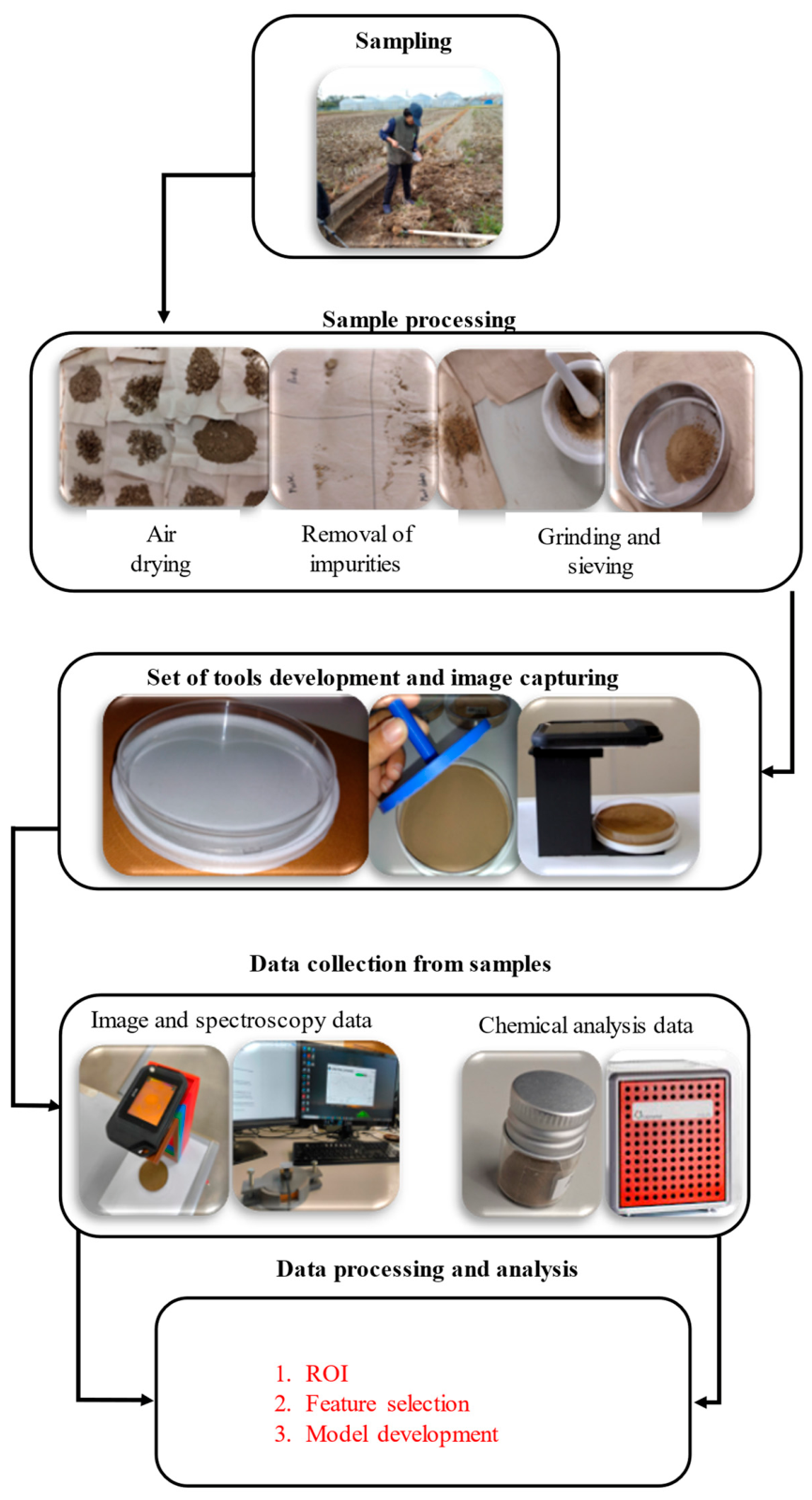
This research was divided into several sections: first, soil was sampled and processed. Then, the data (RGB and thermal images, spectral data) were recorded. Finally, a sub-sample from the processed soil was sent to an accredited laboratory for parallel chemical SOC analysis.

2.1. Soil Sampling and Analysis

Soil samples were collected from 0.2 ha of rice paddy fields located within the Tsukuba Plant Innovation Research Center, Japan, during April and September 2024. The Koshihikari rice variety is grown in a yearly monocropping pattern in Japan from April to November. Soil samples were randomly collected from 0–20 cm depth and prepared for analysis.
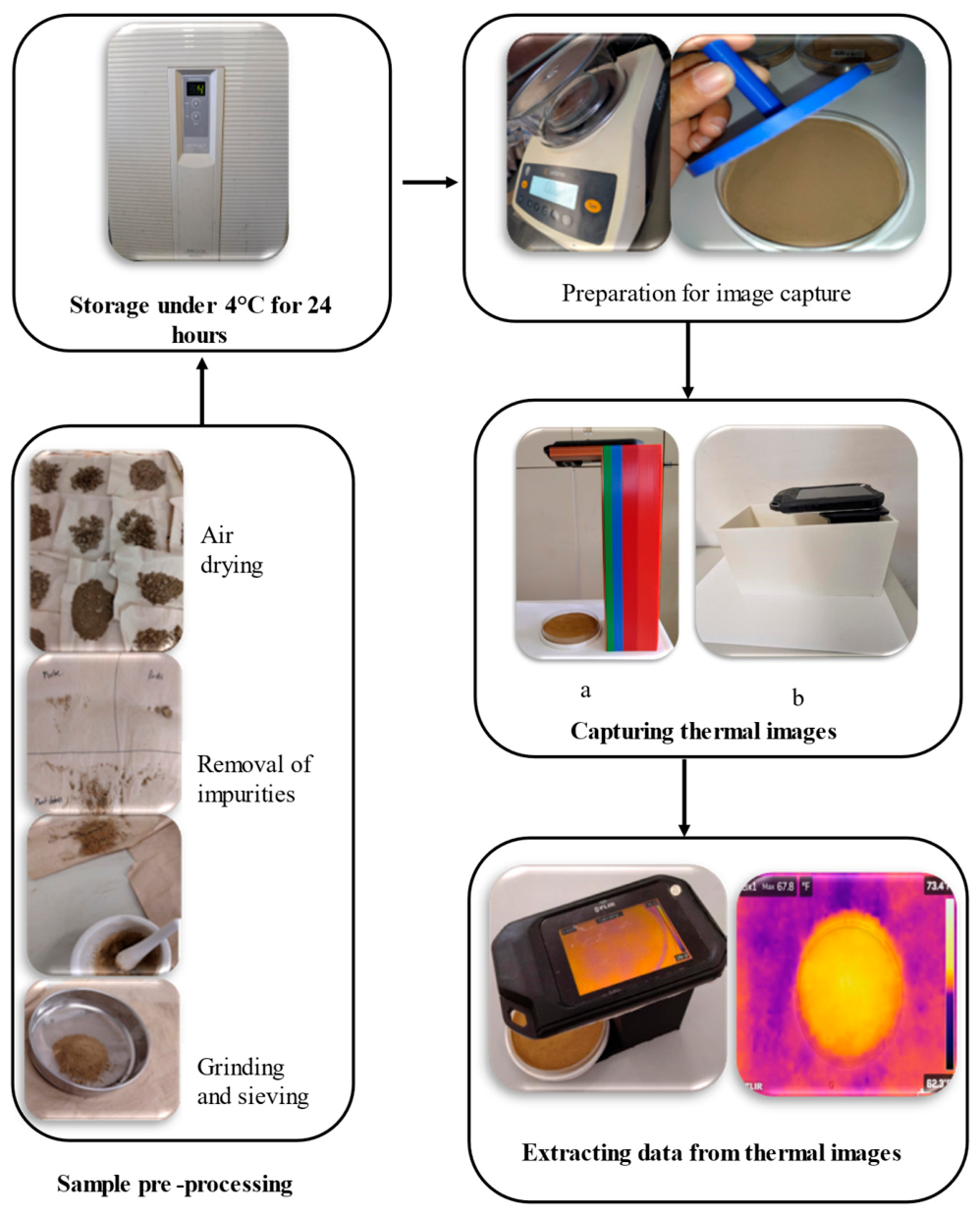
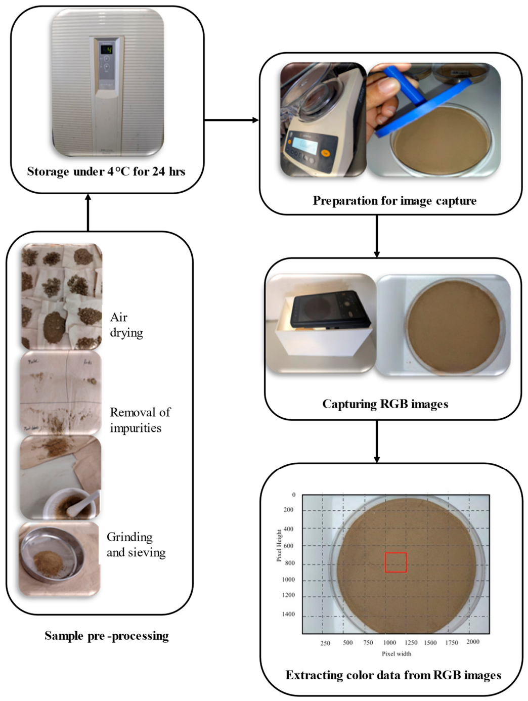
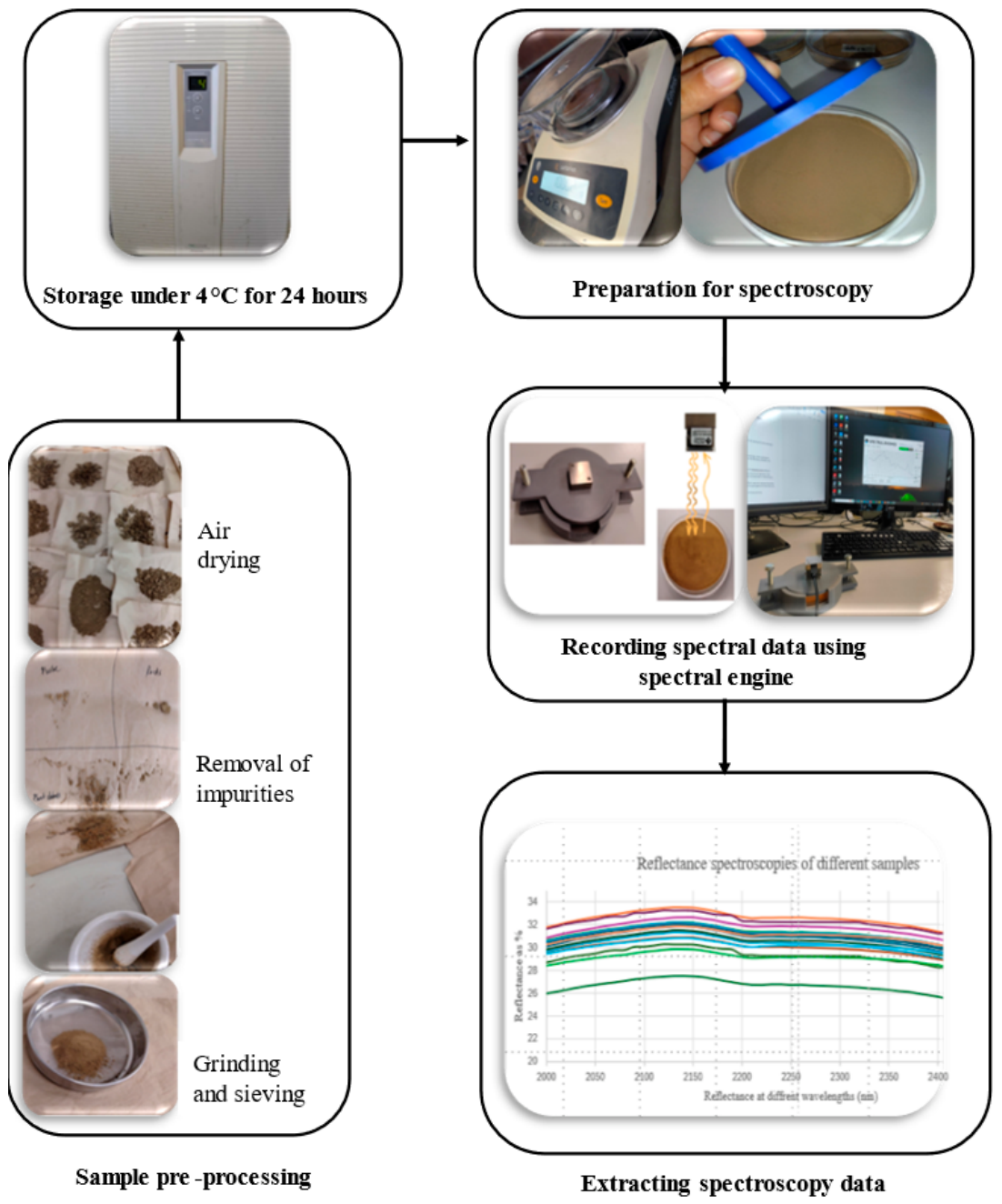
Sample processing included air drying to reduce the moisture below 10%, and portion of the dry sample was analyzed using gravimetric method to ensure dryness. Then the samples were sorted, and non-soil matter was removed (soil coarse fraction; particles larger than 2 mm, plastic residue, plant and animal residues). Then, the samples were ground using a mortar and pestle and sieved through a 0.2 mm standard sieve (Figure 1). Samples were only used to develop models and predict SOC. At this stage of the study, samples were considered as series of known samples to identify correlation with SOC to develop models and were not used for predicting soil conditions of rice paddy fields. This process is shown in Figure 1.
First, data were recorded from the processed soil samples, then sub soil samples (4 g) from each Petri dish were sent to an accredited chemical facility affiliated with the University of Tsukuba. The chemical analysis division, a research center for science and technology, uses UNICUBE (Elementar Analysensysteme GmbH, Langenselbold, Germany) elemental analysis to quantify the SOC values via dry combustion methods. An acid pretreatment of each sample was performed before determining the amount of organic carbon. The SOC data from chemical analysis and spectral data from the spectral engine were subsequently used to identify correlation via statistical analysis.

2.1.1. Thermal Image Processing and Analysis

During the initial stage, 12 randomly collected soil samples from rice fields were analyzed alongside several additional reference samples to investigate the behavior of thermal images in relation to soil organic carbon (SOC). The samples were first processed and stored in a refrigerator at 4 °C. This temperature is regarded as the optimal level for the reduction in microbial activity and is considered suitable for the short- to mid-term storage of soil samples [16,17]. After 24 h, 6 g of soil was transferred to Petri dishes, and thermal (infrared, IR) images were recorded under indoor conditions (uncontrolled).
Thermal images from air-dried samples were recorded using an FLIR C3 (Teledyne FLIR, Wilsonville, OR, USA) thermal camera (IR sensor 80 × 60; thermal sensitivity/NETD < 0.10 °C; image frequency 9 Hz; spectral range 7.5–14.0 µm; −10–150 °C object temperature range). Regarding emissivity, matte nonglossy condition was selected for all images. Images were captured using 25 cm stand (Figure 2a) to hold the camera to avoid differences due to distance. Samples were placed on top of a white sheet, and each sample was placed in the same positions. This was the primary study conducted to understand the correlation between SOC data and the thermal image properties. The process of image collection is shown in Figure 2.
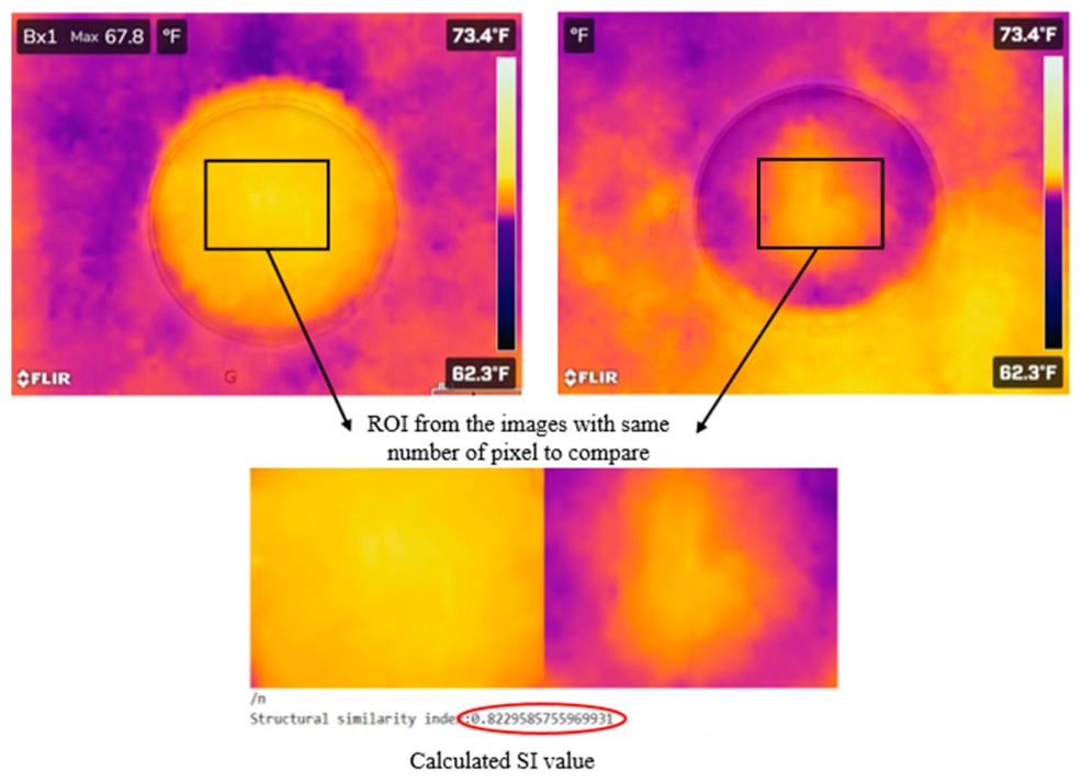
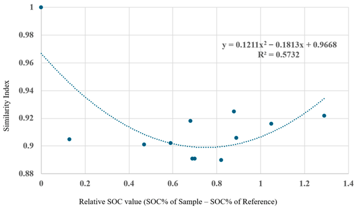
In the preliminary study, in addition to considering individual thermal image data, 12 rice field soil samples were compared with 8 reference samples using the captured thermal images to calculate the similarity index (SI) (Figure 3).
Then, the SI value with relative SOC change (where a positive SOC value difference between the sample being considered and the reference sample is used) was used to identify relationships to develop the SOC prediction model. During the second stage, 16 samples were sampled and preprocessed using the same procedure. Here, we reduced the distance from the soil to the camera further by using a 10 cm stand (Figure 2b) and increased the size of the soil samples from 6 g to 10 g. A white plastic box (3D printed) was used to hold the soil samples, and the camera stand while the images were being taken. With the use of Open-source computer vision (OpenCV (4.13.0) libraries in Python (3.10.12), thermal images were edited to resize the images without losing their properties using the region of interest (ROI) feature.
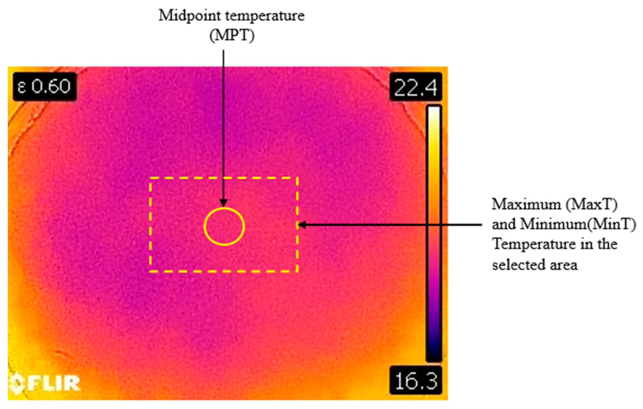
The analysis was conducted using the temperature data from the ROI of the thermal images (Figure 4), and here, compatible software (https://ignite.flir.com) was used to extract the midpoint temperature (MPT), minimum temperature (MinT), and maximum temperature (MaxT) for each sample IR image’s ROI.

2.1.2. Spectroscopy-Based Analysis

The same samples (used for RGB image recording and thermal image recording) were used to record reflectivity data using the NIRONE S2.5 (M-U-T GMBH, Wedel, Germany) spectral engine (spectral range: 2000–2450 nm; light source: built-in tungsten filament). The sensor was able to measure absorbance and reflectance data in the range of 2000 to 2450 nm. Reflectance data were collected at 10 nm intervals, and the average of three readings was used for analysis. The system was calibrated using a white reference and an auto-lamp with dark subtraction; the unit now automatically measures a new dark signal for each calibration. Here, we used a spectral engine holder and soil in a Petri dish. The spectral engine touched the soil but was not buried in the soil (Figure 5).

2.1.3. RGB Image Recording and Analysis

Red, green, and blue (RGB) images consist of pixels specified by the amounts of red, blue, and green and create a color with three coordinates [18]. All the images were captured using a primary Sony Ace III smartphone camera (13 megapixels, ƒ/1.8, and an ISO setting of 166) to ensure hardware consistency. To control the influence of ambient lighting and stabilize the camera’s auto-white balance, image acquisition was conducted in a controlled environment utilizing a full-spectrum LED light source (color temperature: 4323 K; illuminance: 2151 lux) fixed at a distance of 10 cm from the samples. And the camera stands and samples were kept inside a control box (white in color).
The soil samples corresponded to Muncel Soil Color Chart (MSCC) values of 7.5YR3/3. Therefore, a smartphone camera was used to record the image, and then Numerical Python (NumPy) libraries were used to calculate average values for three color models: hue saturation value (HSV); red, blue, and green (RGB) values; and Commission Internationale de l’Eclairage’ (CIE) lightness (L) (green (−a) to red (+a), blue (−b) to yellow (+b)) or CIELab [19]. We used a region of interest (ROI) function to select color from each image to avoid errors associated with the sample container and background color alteration (Figure 6).
The individual values from the color models and SOC values were subsequently subject to feature selection analysis to develop equations for a prediction model.

2.2. Multimodal Sensing Data Integration for SOC Quantification

Since we wanted to consider a model that used a limited number of soil samples for calibration, as well as individual sensor data-based correlation analysis, our focus was on developing a model that fused data from different systems. Further, cost of instruments (spectral engine: 0.45 million JPY; thermal camera: 0.1 million JPY) was also considered for the integration. Since smartphones are available for personal use, we considered RGB images along with each of above high-cost instruments.

2.2.1. Integration of RGB Image and Spectroscopy Data

In this stage, we used the data recorded from the spectral engine and the data from the RGB images to identify relationships with the SOC. Firstly, feature selection (F_regression) was performed by evaluating the significance and importance of all the variables in predicting the response variable (Y or SOC for the study). The variables of highest importance (p values and R2 values) were then selected for further analysis.
The values obtained from the color models and reflectance values (based on feature selection p values) analyzed over the SOC (with the H value from the HSV model and the ‘a’ value from the CIE Lab model; reflectance data spanned intervals from 2150 nm to 2300 nm) were used to develop a model to calculate the SOC values. Resulting model’s R2 values were not strong enough (R2 < 0.5) to use it further.

2.2.2. Integration of RGB Images and IR Images

The values obtained from the color models and the temperature values of the thermal image were individually compared with the SOC, the H value from the HSV model, and the MaxT from the thermal images. This analysis enabled the identification of a polynomial relationship with the SOC. Feature selection was used to understand the significance of 12 representative X values: R, G, B, H, S, V, L, a, b, MPT, MinT, and MaxT. Finally, the coefficient value for each variable and the R2 value were progressively used to evaluate ideal X values to develop a model to predict the SOC.
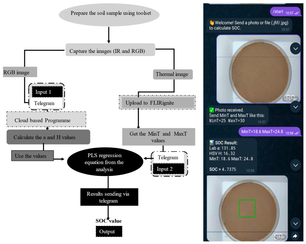
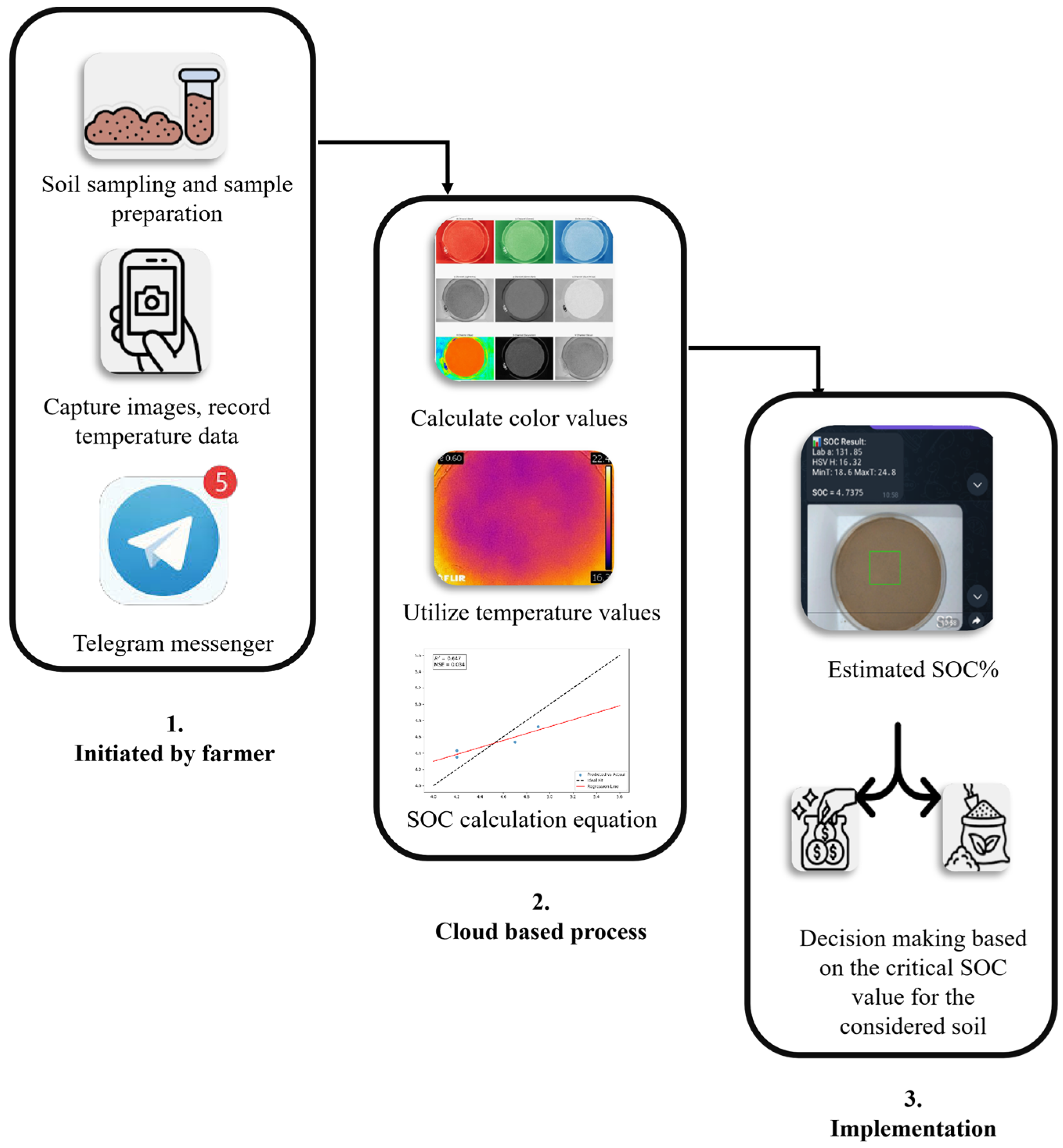
Then, on the basis of the regression model and using Google Colab IDE with Telegram messenger (v12.6.4 user interface), we created a farmer feedback model requiring only a limited number of known samples to estimate the SOC (Figure 6). Google Colab is a hosted Jupiter notebook service that has free access to computing resources and does not require a special setup to run (https://colab.google). Telegram Messenger is a cloud-based software program that provides instant messaging and social media services (https://telegram.org/). Our goal was to make customized models that were available to farmers at no cost. Step-by-step guidelines are illustrated in Figure 7.
This model includes a program to predict the SOC from RGB image and IR image data via a computational tool. This system uses two sensor-based datasets that farmers utilize through the Telegram messenger platform, in which an automated analysis script processes the inputs. The analysis follows a sequential multistep data acquisition and workflow process (Algorithms 1–4).
Algorithm 1: Main Event-Driven Logic
Users start by sending the ‘/start’ command to the system, and upon receiving the command script, they encounter the welcome message and the step-to-step guide to submit input data starting with the image captured by the smartphone.
PROCEDURE Main
BEGIN
REGISTER HANDLER for command “/start” to execute Procedure Handle_Start
REGISTER HANDLER for incoming “photo” messages to execute Procedure Handle_Image
REGISTER HANDLER for incoming “text” messages to execute Procedure Handle_Text
START POLLING for events
MAINTAIN IDLE state
END
Algorithm 2: Image processing
Upon receiving the image, the system enters a temporary state and waits for the other data submissions. Here, the system sends a request to the user to submit the MinT and MaxT from the IR image with an example guide text. These data are directly taken for the calculation of the SOC, and they are integral parts of the equation.
PROCEDURE Handle_Image(incoming_photo_message)
BEGIN
GET user_id FROM incoming_photo_message
SET local_image_path = GENERATE_UNIQUE_PATH_FOR_USER(user_id)
GET photo_file = SELECT_HIGHEST_RESOLUTION(incoming_photo_message)
DOWNLOAD photo_file TO local_image_path
CALL Store_Session_State(user_id, local_image_path)
SET prompt_message = “Image received. Please provide ancillary data in the format: MinT = 25 MaxT = 30”
SEND_MESSAGE (to user_id, with prompt_message)
END
Algorithm 3: Secondary data handling and computation
Once all the inputs are received, the system starts the calculation of the SOC. This involves converting the RGB image to an HSV value and employing the CIE Lab models, which selects of ROI, calculates the average “H” and “a” values from the ROI area. These two values with MinT and MaxT are subsequently used by the system to compute the SOC via the equation.
PROCEDURE Handle_Text(incoming_text_message)
BEGIN
GET user_id FROM incoming_text_message
GET text_content FROM incoming_text_message
SET session = Retrieve_Session_State(user_id)
IF session is NULL THEN
SEND_MESSAGE (to user_id, with “Error: Please send an image first.”)
RETURN
END IF
TRY
SET MinT = PARSE_NUMERIC_VALUE (from text_content, for key “MinT”)
SET MaxT = PARSE_NUMERIC_VALUE(from text_content, for key “MaxT”)
SET image_path = session.image_path
SET a, H, SOC, roi_path = CALL Compute_SOC_and_Image(image_path, MinT, MaxT)
SET result_text = FORMAT_RESULTS(a, H, MinT, MaxT, SOC)
SEND_MESSAGE(to user_id, with result_text)
SEND_PHOTO(to user_id, from roi_path)
CALL Delete_Session_State(user_id)
CATCH ParsingError
SET error_message = “Error parsing input. Use format: MinT = 25 MaxT = 30”
SEND_MESSAGE(to user_id, with error_message)
END TRY
END
Algorithm 4: SOC estimation and image handling
After the calculation is complete, together with the information of the data used to calculate the SOC and an image with the ROI, the calculated SOC is sent to the user via the automated analysis script.
PROCEDURE Compute_SOC_and_Image (image_path, MinT, MaxT)
BEGIN
SET img = READ_IMAGE_FROM_PATH(image_path)
SET lab_image = CONVERT_COLOR(img, from BGR to LAB)
SET hsv_image = CONVERT_COLOR(img, from BGR to HSV)
SET lab_roi = EXTRACT_REGION(lab_image, x_start, y_start, x_end, y_end)
SET hsv_roi = EXTRACT_REGION(hsv_image, x_start, y_start, x_end, y_end)
SET a_mean = CALCULATE_MEAN(channel ‘a’ of lab_roi)
SET H_mean = CALCULATE_MEAN(channel ‘H’ of hsv_roi)
CALCULATE ‘PLS regression equation for SOC’
DRAW_RECTANGLE(img, from (x_start, y_start) to (x_end, y_end))
SET result_img_path = GENERATE_PATH(image_path, suffix: “_roi”)
SAVE_IMAGE(img, to result_img_path)
SET data_record = [image_path, MinT, MaxT, a_mean, H_mean, SOC]
APPEND_RECORD_TO_CSV(“soc_results.csv”, data_record)
RETURN a_mean, H_mean, SOC, result_img_path
END

2.3. Instrument Design and Fabrication

This methodology involves data recording from soil samples and comparisons. Therefore, to ensure comparability, simplicity, and control of light- and height-related errors, it was necessary to provide guidelines and simple tools. Accordingly, in parallel with our planning of the analysis, we developed a set of new tools using 3D printing with low-cost materials. The imaging and spectroscopy data acquisition methodologies employed in earlier studies did not include information on surface conditions or on how they smoothed out soil layers for data collection.
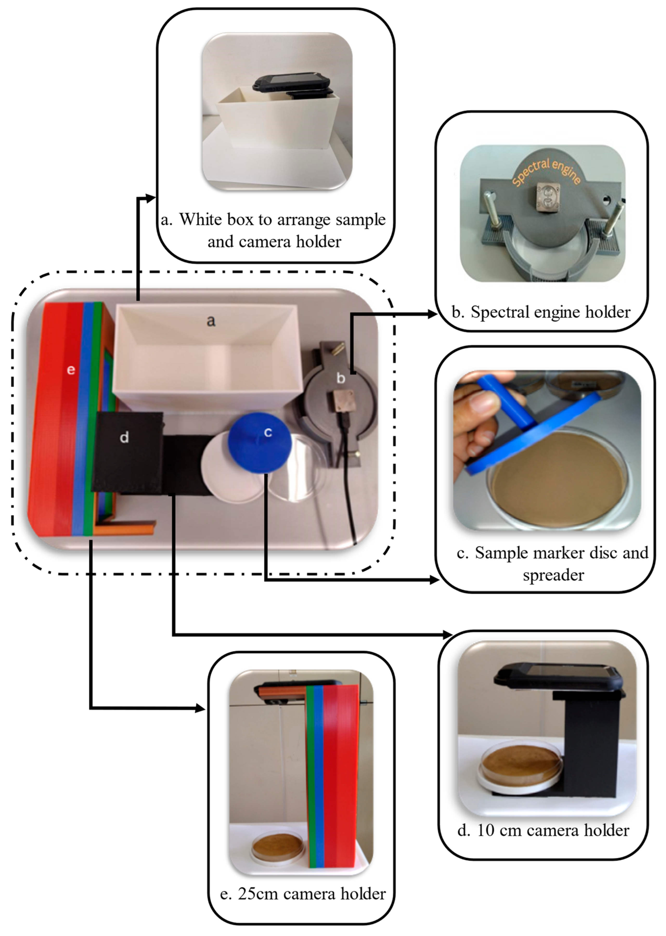
This process yielded six tools (Figure 8): (a) A white box was used to retain the sample during RGB image capture to prevent as much light as possible from coming in, (b) The soil sample holder The NIR sensor holder was designed to set the standard distance between the sensor and the soil layer (gray), (c) are the sample holder and spreader (blue) which are used to make soil layer. Height of the sample holder was chosen to use as a marker to ensure thickness of soil layer inside the Petri dish (d) and (e) are two different holders were designed to capture the IR image and RGB images of the soil sample from heights of 25 cm and 10 cm to set the distances between the camera and the sample.

3. Results

The results of the SOC analysis can be divided into main categories on the basis of which sensor was used to obtain data from the processed soil samples.

3.1. Soil Sampling Analysis

The following section presents the SOC data for the sample under consideration, as determined by chemical analysis (Table 1).

3.1.1. Thermal (IR) Images and SOC

Initially, we aimed to assess the significance of variations among the thermal images. Using Numerical Python library, differences between the image datasets were computed; however, the model initially interpreted these images as highly similar. Subsequently, the similarity index (SI) was calculated using NumPy-based algorithms to quantitatively evaluate the degree of similarity between the thermal images. The similarity index (SI), or structural similarity index, is a methodology developed by Wang et al. [20] to analyze the similarity of two images via an algorithm. The similarity index values range from 0% (completely different) to 100% (completely similar). To calculate the similarity index (SI), it was essential to first identify the most appropriate reference image. This was achieved by considering differences in soil organic carbon (SOC) levels among the samples. These reference samples included upland soil samples with low levels of SOC (1.96% to 3.61%), coral sand (MSCC white page 2.5Y 9/1 with 11.21%) samples with more carbonate carbon, and a rice husk biochar (MSCC 10YR 2/1 20.45%) sample. For instance, rice husk biochar (RHB), which exhibits relatively high SOC levels, was compared with rice field soil samples and upland soil samples, which have comparatively lower SOC values. The objective was to evaluate the correlation between image similarity and SI and subsequently use this relationship as a basis for developing a model to predict SOC content.
The highest correlation identified in the study was the SI values calculated for the paddy field samples with the paddy field sample (with lowest SOC) as a reference. The two-order polynomial relationship is shown in Figure 9, and the R2 value for the model was 0.57.
Apart from SI, three parameters extracted from the IR images that were used in the analysis were MPT, MinT, and MaxT, which were evaluated for SOC prediction. The calculated feature selection (F_regression) p values were larger than 0.05.

3.1.2. Reflectance Data from the Spectral Engine

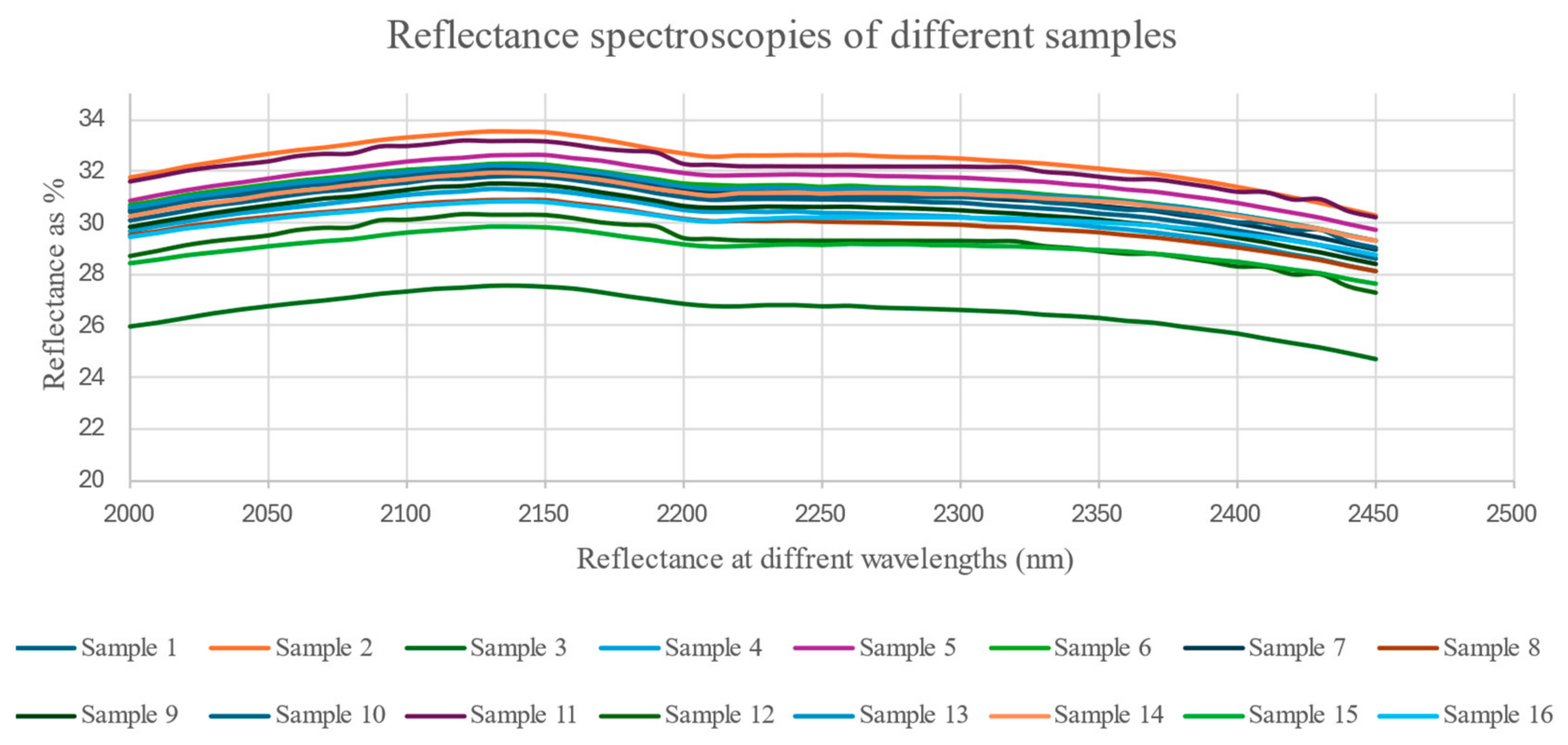
During the experiment, the reflectance data were collected from 2000 to 2450 nm with 10 nm intervals. The recorded reflectance data for 16 samples is shown in Figure 10. The datasets from these samples did not show strong enough co-linearity to develop a prediction model.

3.1.3. RGB Image Analysis

The significance of the relationship with individual values of each color model’s SOC was studied, and there was no significant correlation for a prediction model under the considered number of samples (p > 0.05 during p-value-based feature selection; F_regression).

3.2. Multi-Model Sensing Integration for SOC Determination

Since the identified relationships from the individual sensor datasets (IR image data, temperature, and SI; RGB image data: values from color models) with SOC data did not yield significant enough correlation possibilities (above 0.6 model fit R2 values) to use in a prediction model, we integrated data from individual models. Then, we focused on developing a multimodal prediction model with a minimum number of samples.
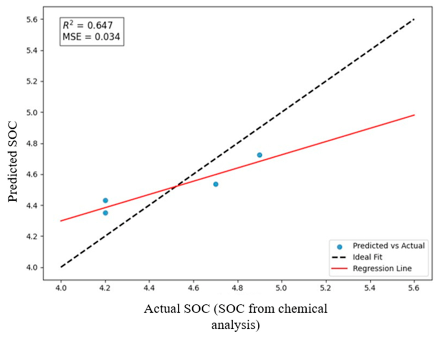
The data were analyzed using Python (3.10.12) and Microsoft Excel, and graphical figures were generated via math plot libraries. After the data from these two types of images were considered, we were able to predict the SOC with the PLS model, which had an R2 of 0.647 and an MSE of 0.034 (Figure 11). A partial least square regression model (PLS) analysis was conducted to develop the equation. Finally, one model was used to predict the SOC as a cloud-based application initiated via the Telegram messenger command.
The regression line matched the actual data at an SOC value of approximately 4.5, with lower predicted values above 5% (Figure 11). The variables used for X were from the color models; ‘a’ and ‘H’ were from the thermal image; and MinT, MaxT, and Y are the dependent SOC variables (Equation (1)).
S O C = 43.9205 + 0.0672 × M i n T + 0.1146 × M a x T + ( 0.3420 × a + 0.1209 × H )
Considering the four sample outcomes from the model and cross-validation with laboratory analysis, we evaluated the acceptability of the SOC value calculated via the new method. We conducted a paired sample t-test to determine whether the SOC values from the two analysis methods were significantly different (Table 2).
For these values, the calculated t value was 2.7094 and the critical value was 3.182, using a 95% confidence level and three degrees of freedom. Therefore, the values calculated via the new method and the SOC values from the chemical analysis were not significantly different for these samples. The accuracy was best near the mean SOC value of 4.6%, and going further from the mean SOC value led to greater deviation from the measured value.

4. Discussion

Individual sensor datasets, including infrared (IR) imagery (temperature and similarity index (SI)), RGB color model values, and spectral reflectance (2000–2450 nm), showed weak correlations with soil organic carbon (SOC) data as the p-values for feature selection (F_regression value) remained high. Consequently, we employed data fusion, integrating sensors and camera imagery to develop a prediction model optimized for a limited sample size. Since the F_regression provides p and R2 values for individual variables [21], these values were considered variables of importance in model prediction and were used in multimodal sensing. Throughout data collection, we used the same samples in Petri dishes to improve the comparability of multimodal data.
During our research, we used three sensors: a spectral engine, a thermal camera, and a smartphone camera. IR images were developed to capture images based on their unique emissivity. According to Kirchhoff’s Law of thermal radiation [22], the following is obtained (Equation (2)):
T +   R +   E   = 1
where R, T, and E represent reflectance, transmittance, and emissivity, respectively. In the context of thermal imaging systems, the emissivity coefficient was selected from the device (i.e., the FLIR C3 camera) in order to ensure the comparability of thermographic measurements. We set up the emissivity based on the nature of the material before capturing the images (the model has four options: matte, semi-matte, semi-glossy, and custom value). Therefore, for the collected images, we kept the emissivity as matte, thus increasing the reflectivity (R) and reducing T (if the surface conditions are similar, dark-colored soil is less reflective).
The spectral engine utilized an integrated light source to measure the reflectance and absorbance data within the 2000–2450 nm range from the soil samples. This specific spectral band was selected based on the established accuracy of previous research using near-infrared (NIR) and mid-infrared (MIR) spectroscopy for soil organic carbon (SOC) detection [5]. Furthermore, the selection process prioritized model compatibility with Internet of Things (IoT) frameworks and cost efficiency, ensuring the development of an affordable solution suitable for farm-level deployment.
Smartphone cameras, like other basic cameras, mimic the human eye in the digital world. These cameras record values from the visible spectrum (450 nm to 700 nm) to form an RGB image [18]. We used RGB images with either a spectral engine or a thermal camera in combination to avoid the higher cost associated with combining two IR sensors and to increase user friendliness. The soil we used was Gray lowland soil [23], and the 16 samples considered had the same Munsell soil color chart (MSCC) value of 10YR5/2. The color charts used in this study consisted of 450 chips from the 2009 revised edition, produced in 2024. These charts correspond to the Munsell Soil Color Charts manufactured by Munsell Color.
Recent advancements in proximal soil sensing have demonstrated the potential of digital image-based analysis to offer cost-effective alternatives to traditional laboratory methods [24,25]. The utilization of open-source computer vision libraries, such as OpenCV, has enabled researchers to extract textural and color features of soil that correlate with soil nutrient data [26].
Regarding the statistical analysis, we initially focused on a regression analysis, and for the regression analysis, X was applied such that the other factor was considered the dependent factor (Y). A regression analysis can be used to construct a calibration graph. Nonlinear higher-order relationships are also possible, and these relationships are more complex to analyze mathematically [27]. This study evaluated multiple modeling approaches, beginning with a linear regression and extending to a Lasso regression, and polynomial regression analyses. Based on model fit metrics and the assessment of multicollinearity among predictor variables, the partial least squares (PLS) regression model was identified as the most suitable for the given dataset. Compared with other statistical methods, the suitability of PLS regression analysis in spectroscopy-based SOC analysis has also been discussed in previous research [3,5,28].

4.1. Color Models and SOC Prediction

A material or object’s distinctive attributes can be characterized by its color [29]. Color models based on the MSCC can be used to provide soil color-associated information, including the SOC. Several studies have been conducted to use these models to predict the SOC. Some of the studies have produced reliable predictions, but the equations used differ across studies, indicating the unavailability of a universal equation. In previous studies, lightness (L) has been identified as a predictor of SOC [19,30,31]. Additionally, the value (V) in the HSV model is associated with SOC changes, and the potential of V as a predictor has been reported [19,31,32]. Some of the identified relationships with the RGB image data and SOC from the previous literature can be described as follows (Table 3).
The models from the previous research mentioned above have obtained higher accuracy levels with the increasing number of samples used. However, an edge application has not yet been developed for use in farming systems.
Three color models were considered in the present study: CIE Lab, RGB, and HSV. The models were able to provide nine variables for the X-axis to predict the SOC as the Y value. However, the reported data from the analyses were not enough to develop models with agreeable accuracy (the R2 values were less than 0.6). Further, the F_regression data did not support the lightness-related variables or value-related variables in the model for the considered set of samples.

4.2. Thermal Image Data and SOC Prediction

Compared with digital images, IR images and NIR spectroscopy can capture more of the details of a material. This detailed information can be used for analysis in the border context, and these methodologies can be used to replace high-cost laboratory analysis [32]. IR images are used in remote sensing and moisture data recording. Initially, we examined the thermal data using the SI to develop an SOC prediction model, and we observed a polynomial relationship. There is a possibility that the relationship would not be improved in a new set of images due to changes in image capturing distance and thickness; therefore, further studies are needed. Furthermore, we also used temperature data from the ROI of the IR images to study the relationship with the SOC. The analysis results were not strong enough to provide mathematical models to predict SOC using these data series.

4.3. Spectroscopy Data and SOC Analysis

Spectral analysis has been used for several decades to provide data on soil samples, but the application of SOC analysis still needs to be developed. Spectrophotometers have a built-in light source, but they can record measurements throughout the spectrum and provide the ratio between the light reflected from a sample and that from a calibrated working standard. The NIRONE S2.5 spectral engine we used in the experiment was able to record reflectance or absorbance data in the range of 2000 nm to 2300 nm, and we determined that the sensitivity was greater in the range of 2150 nm to 2300 nm compared to other ranges (based on F_regression R2 values). Narrowing down the spectral range is necessary when developing an edge device.

4.4. Multimodal Analysis with Integration of Sensors

The ability of this model to predict soil with an SOC of approximately 1% is significant when a small number of known samples (16) are used; this method combines two sensors (a smartphone camera and a thermal camera) and has an R2 of 0.62. Compared to previous studies, the reduction in the number of known samples is an advantage in this study, since the required number for the majority of available spectroscopy-based and image-based SOC prediction methods is more than 100 samples. Table 4 presents a summary of some of the previous work, the number of samples used, and the soil sample SOC range. We collected samples from 0.2 ha of land (one unit) used for paddy cultivation, where color and SOC changes were limited. Therefore, further research into different types of soil needs to be conducted to ensure model performance and applicability to small fields.

4.5. Implementation of the Developed Method and Applications of the SOC Value

According to Jamaluddin et al. [35], in regard to the digital literacy of farmers aged 31 years or above, 50% of them are categorized as having low digital literacy. They most commonly use digital technologies on their smartphones (90%), while the use of the internet of things (IoT) (50%) and decision support apps (15%) is lower. Therefore, this methodology focuses on farmers using smartphones or farmer organizations/communities with supportive, digitally literate extension staff. Furthermore, the use of SOC analysis data can serve several purposes in agricultural systems, such as irrigation scheduling, tillage control, and the addition of organic fertilizers, with potential for carbon sequestration and carbon credits.

4.6. Application of SOC Data

Research has revealed that yield increases with increasing soil organic carbon (SOC) until the mean optimum soil carbon is reached [36]. Therefore, the SOC value can be used to control the amount of organic fertilizer applied. SOC also has an optimum level below which soil degradation and productivity loss occur. Patric et al. suggested that the lower threshold is as low as 2% in 2013. Further, when SOC is below 0.75%, the soil is considered ‘depleted,’ with a limited ability to retain nutrients or support microbial structures. These very low levels also pose a high risk of erosion and compaction, necessitating restoration. Low SOC levels (0.75–1.5%) result in reduced biological and physical functioning, leading to lower productivity caused by recent degradation or a history of low inputs. SOC levels of 1.6–2.5% are considered adequate for moderate productivity, though they require continued carbon inputs to achieve long-term sustainability. Most of the world’s soils fall into this medium category. Levels of 2.6–3.5% are considered high; such fertile soils are biologically active and support resilient cropping systems. Finally, very high SOC levels (>3.5%) facilitate carbon sequestration and provide ecosystem services that extend beyond crop production [37,38,39]. However, the value can change based on the soil texture and structure. Therefore, when farmers see that their SOC values are categorized as low and depleted, they can make the decision to apply organic fertilizers to improve productivity, and if the calculated value is high or very high, they can avoid the costs associated with organic fertilizer applications. Additionally, tillage and mulching can improve the SOC value in SOC-deficient soil. Studies have shown that tillage and mulching significantly influence the SOC concentration [40]. Additionally, in 2006, Alvarez [41] reported that rainwater infiltration control improvement and SOC level increases can be achieved by tillage control. This is a sustainable option to improve water use efficiency while improving SOC. The availability of excess SOC can cause environmental degradation. The application of these operations can be guided by the SOC values to improve soil conditions. In this instance, site-specific factors are likely to exert a significant influence; consequently, it is imperative to consult with experts who are able to take into account the prevailing local conditions.
The addition of organic matter to meet an optimum SOC level improves soil biodiversity and improves pore space, leading to better infiltration and less water runoff [42]. Precision irrigation systems can be used to manage the water in the soil to ensure the availability of optimal amounts of water to crops without waste, which is important for sustaining all plant physiological processes [43]. SOC improves the water holding capacity and water use efficiency, so the SOC value has the potential to be used as an indicator to fine-tune irrigation practices along with other factors. In brief, we can use the proposed model to improve system efficiency (Figure 12).

5. Conclusions

There is no universal equation for color-based models or spectroscopy-based models; different soils have different relationships, so it is important to find methodologies to develop models with a minimum number of known samples with a reasonable accuracy for specific soils in order to analyze farmers’ fields. Compared with data collected from soil samples via one type of sensor or camera, the incorporation of two sensors has the potential to improve model fitness and reduce the number of known samples needed.
A new model was developed with the data collected from RGB images and IR images:
  • We were able to develop an SOC analysis method with reasonable accuracy (1% change in soil samples near the model’s mean value of SOC);
  • Combining data from thermal images and RGB images provides the potential to predict the SOC values of samples with similar MSCC colors with smaller SOC variations;
  • The process can be customized for individual farmers with digital literacy to conduct self-analyses in their fields.
A limitation of the current study is the reliance on a single smartphone model under controlled lighting conditions. Different smartphone cameras utilize varying image signal processors (ISPs) that apply proprietary color and contrast enhancements. Future development of this system for broader commercial use will necessitate the inclusion of a standardized color reference (such as a 50% gray card) within the camera’s field of view. This will allow for the mathematical normalization of RGB values, ensuring color constancy and reliable results regardless of the smartphone hardware or ambient lighting conditions. The authors strongly recommend the customization of models for farmers using available resources (their own mobile phones or a thermal camera). Further research involving model suitability tests using soil types with different colors and land use types needs to be conducted.

Author Contributions

Conceptualization, N.S.L.S., methodology, N.S.L.S. and P.C.; formal analysis, N.S.L.S.; writing—original draft preparation, N.S.L.S.; writing—review and editing, T.A.; visualization, N.S.L.S.; supervision, T.A.; writing—review and editing, conceptualization, T.A. All authors have read and agreed to the published version of the manuscript.

Funding

This research was funded by JSTSPRING program, grant number JPMJSP2124.

Institutional Review Board Statement

Not applicable.

Informed Consent Statement

Not applicable.

Data Availability Statement

The collected data belongs to an ongoing study and can be made available upon reasonable request.

Acknowledgments

The authors are grateful for the JST-SPRING fellowship and the Tsukuba Plant Innovation Research Center (TPIRC), University of Tsukuba for providing the research facilities used.

Conflicts of Interest

The authors declare no conflicts of interest. The founders had no role in the design of the study; in the collection, analyses, or interpretation of data; in the writing of the manuscript; or in the decision to publish the results.

References

  1. International Atomic Energy Agency. Agricultural Water Management. Joint FAO/IAEA Programme; Nuclear Techniques in Food and Agriculture. December 2024. Available online: https://www.iaea.org/topics/agricultural-water-management (accessed on 6 February 2025).
  2. Suchitra, M.S.; Pai, M.A. Improving the prediction accuracy of soil nutrient classification by optimizing extreme learning machine parameters. Inf. Process. Agric. 2019, 7, 72–81. [Google Scholar] [CrossRef] [Scilit]
  3. McCarty, G.W.; Reeves, J.B.; Reeves, V.B.; Follett, R.F.; Kimble, J.M. Mid-infrared and near-infrared diffuse reflectance spectroscopy for soil carbon measurements. Soil Sci. Soc. Am. J. 2002, 66, 640–646. [Google Scholar] [CrossRef] [Scilit]
  4. Anglopoulou, T.; Tziolas, N.; Balafoutis, A.; Zalidis, G.; Bochtis, D. Remote Sensing Techniques for Soil Organic Carbon Estimation: A Review. Remote Sens. 2019, 11, 676. [Google Scholar] [CrossRef] [Scilit]
  5. Loria, N.; Lal, R.; Chandra, R. Handheld in Situ Methods for Soil Organic Carbon Assessment. Sustainability 2024, 16, 5592. [Google Scholar] [CrossRef] [Scilit]
  6. Zhou, T.; Geng, Y.; Lv, W.; Xiao, S.; Zhang, P.; Xu, X.; Chen, J.; Wu, Z.; Pan, J.; Si, B.; et al. Effects of optical and radar satellite observations within Google Earth Engine on soil organic carbon prediction models in Spain. J. Environ. Manag. 2023, 338, 117810. [Google Scholar] [CrossRef] [Scilit]
  7. Kabiri, S.; O’Rourke, S.M. Coarse to superfine: Can hyperspectral soil organic carbon models predict higher-resolution information? Front. Environ. Sci. 2024, 12, 1392469. [Google Scholar] [CrossRef] [Scilit]
  8. Ou, J.; Wu, Z.; Yan, Q.; Feng, X.; Zhao, Z. Improving soil organic carbon mapping in farmlands using machine learning models and complex cropping system information. Environ. Sci. Eur. 2024, 36, 80. [Google Scholar] [CrossRef] [Scilit]
  9. Islam, S.F.; Van Groenigen, J.W.; Jensen, L.S.; Sander, B.O.; De Neergaard, A. The effective mitigation of greenhouse gas emissions from rice paddies without compromising yield by early-season drainage. Sci. Total Environ. 2018, 612, 1329–1339. [Google Scholar] [CrossRef] [Scilit]
  10. Xiao, Y.; Huang, R.; Zhang, Z.; Wong, V.N.L.; Li, X.; Tang, X.; Luo, Y.; Wu, Y.; Liu, J.; Li, S.; et al. Effects of soil labile carbon fractions and microbes on GHG emissions from flooding to drying in paddy fields. J. Environ. Sci. 2025, 158, 420–434. [Google Scholar] [CrossRef] [Scilit] [PubMed]
  11. USDA. Smart Nutrient Management Save Money and Protect Water Quality, United States of America Department of Agriculture (USDA), Factsheet. 2022; pp. 1–2. Available online: https://www.farmers.gov/sites/default/files/2022-09/farmersgov-fact-sheet-smart-nutr-mgnt-9-2022.pdf (accessed on 21 June 2025).
  12. Saiz-Rubio, V.; Rovira-Mas, F. From Smart Farming towards Agriculture 5.0: A Review on Crop Data Management. Agronomy 2020, 10, 207. [Google Scholar] [CrossRef] [Scilit]
  13. Shepherd, K.D.; Walsh, M. Development of Reflectance Spectral Libraries for Characterization of Soil Properties. Soil Sci. Soc. Am. 2002, 66, 988–998. [Google Scholar] [CrossRef]
  14. Fidêncio, P.H.; Poppi, R.J.; De Andrade, J.C. Determination of organic matter in soils using radial basis function networks and near infrared spectroscopy. Anal. Chim. Acta 2002, 453, 125–134. [Google Scholar] [CrossRef] [Scilit]
  15. Taneja, P.; Vasava, H.K.; Daggupati, P.; Biswas, A. Multi-algorithm comparison to predict soil organic matter and soil moisture content from cell phone images. Geoderma 2021, 385, 114863. [Google Scholar] [CrossRef] [Scilit]
  16. Tian, C.; Cui, D.; Cao, Y.; Luo, S.; Song, H.; Yang, P.; Bai, Y.; Tian, J. Temperature-dependent soil storage: Changes in microbial viability and respiration in semiarid grasslands. Soil Biol. Biochem. 2025, 202, 109673. [Google Scholar] [CrossRef] [Scilit]
  17. Fromin, N. Impacts of soil storage on microbial parameters. Soil 2024, 11, 247–265. [Google Scholar] [CrossRef] [Scilit]
  18. Pinhero, A.; Anupama, M.L.; Vinod, P.; Visaggioc, C.A.; Aneesh, N.; Abhijith, S.; AnanthaKrishnan, S. Malware detection employed by visualization and deep neural network. Comput. Secur. 2021, 105, 102247. [Google Scholar] [CrossRef] [Scilit]
  19. Rossel, R.A.V.; Walter, C.; Fouad, Y. Assessment of two reflectance techniques for the quantification of the within-field spatial variability of soil organic carbon. Precis. Agric. 2003, 697–703. [Google Scholar] [CrossRef] [Scilit]
  20. Wang, Z.h.o.u.; Bovik, A.C.; Sheikh, H.R.; Simoncelli, E.P. Image quality assessment: From error visibility to structural similarity. IEEE Trans. Image Process. 2004, 13, 600–612. [Google Scholar] [CrossRef] [Scilit] [PubMed]
  21. Scikit-Learn Developers. f_regression. In Scikit-Learn Documentation. Available online: https://scikit-learn.org/stable/modules/generated/sklearn.feature_selection.f_regression.html (accessed on 13 June 2024).
  22. Kirchhoff, G.R. Radiative Transfer. California Institute for Technology, 1891; pp. 51–55. Available online: https://web.gps.caltech.edu/~mbrown/classes/ge108/week3/lec6.pdf (accessed on 13 March 2025).
  23. NARO Japan Soil Inventory. 2023. Available online: https://soil-inventory.rad.naro.go.jp/offer.html (accessed on 4 February 2025).
  24. Taneja, P.; Vasava, H.B.; Fathololoumi, S.; Daggupati, P.; Biswas, A. Predicting soil organic matter and soil moisture content from digital camera images: Comparison of regression and machine learning approaches. Can. J. Soil Sci. 2022, 102, 767–784. [Google Scholar] [CrossRef] [Scilit]
  25. Morais, P.A.d.O.; de Souza, D.M.; Madari, B.E.; Soares, A.d.S.; de Oliveira, A.E. Using image analysis to estimate the soil organic carbon content. Microchem. J. 2019, 147, 775–781. [Google Scholar] [CrossRef] [Scilit]
  26. Rajalingam, B.; Mohamed, S.A.; Arshath, A.H.; Dinesh, K.S. Tamil Nadu Seed Image Dataset with OpenCV Preprocessing for Precision Agriculture. Int. J. Sci. Strateg. Manag. Technol. 2026, 2, 1–9. [Google Scholar] [CrossRef] [Scilit]
  27. Food and Agriculture organization (FAO). Basic Statistical Tools. 2023. Available online: https://www.fao.org/4/w7295e/w7295e08.htm (accessed on 20 December 2024).
  28. Senevirathne, N.S.L.; Ahamed, T. Rapid analysis of Soil Organic Carbon in Agricultural Lands: Potential of Integrated Image Processing and Infrared Spectroscopy. AgriEngineering 2024, 6, 3001–3015. [Google Scholar] [CrossRef] [Scilit]
  29. Ibraheem, N.A.; Hasan, M.M.; Khan, R.Z.; Mishra, P.K. Understanding Color Models: A Review. ARPN J. Sci. Technol. 2012, 2, 265–275. Available online: https://www.researchgate.net/publication/266462481 (accessed on 18 December 2024).
  30. Rossel, R.A.V.; Minasny, B.; Roudier, P.; McBratney, A.B. Color space models for soil science. Geoderma 2006, 133, 320–337. [Google Scholar] [CrossRef] [Scilit]
  31. Jorge, N.F.; Clark, J.; Cárdenas, M.L.; Geoghegan, H.; Shannon, V. Measuring soil color to estimate soil organic carbon using a large-scale citizen science-based approach. Sustainability 2021, 13, 11029. [Google Scholar] [CrossRef] [Scilit]
  32. Konen, M.E.; Burras, C.L.; Sandor, J.A. Organic Carbon, Texture, and Quantitative Color Measurement Relationships for Cultivated Soils in North Central Iowa. Soil Sci. Soc. Am. J. 2003, 67, 1823–1830. [Google Scholar] [CrossRef] [Scilit]
  33. Igne, B.; Reeves, J.B., III; MaCarty, G.; Hively, W.D.; Lund, E.; Hurburgh, C.R., Jr. Evaluation of Spectral Pretreatments, Partial Least Squares, Least Squares Support Vector Machines and Locally Weighted Regression for Quantitative Spectroscopic Analysis of Soils. J. Near Infrared Spectrosc. 2010, 18, 167–176. [Google Scholar] [CrossRef] [Scilit]
  34. Fu, Y.; Taneja, P.; Lin, S.; Ji, W.; Adamchuk, V.; Daggupati, P. Asim Biswas Predicting soil organic matter from cellular phone images under varying soil moisture. Geoderma 2020, 361, 114020. [Google Scholar] [CrossRef] [Scilit]
  35. Jamaluddin, S.P.S.; Hati, D.M.; Sahudin, N.A.; Yusof, S.M.; Redzuan, N.A.L.; Ishank, N.A.; Baharin, A.T. Exploring the Level of Digital Literacy and the Adoption of Precision Farming Technologies Among Smallholder Paddy Farmers in Kedah. J. Inf. Syst. Eng. Manag. 2025, 10, 829–843. Available online: https://jisem-journal.com/index.php/journal/article/view/7524/3473 (accessed on 20 January 2025). [CrossRef] [Scilit]
  36. Ma, Y.; Woolf, D.; Fan, M.; Qiao, L.; Li, R.; Lehmann, J. Global crop production increase by soil organic carbon. Nat. Geosci. 2023, 16, 1159–1165. [Google Scholar] [CrossRef] [Scilit]
  37. Parvej, M.R.; Brandt, D.; Myers, R.; Nelson, K.; Singh, G.; Reinbott, T. Soil Organic Carbon: A Foundational Indicator of Soil Health; Extention University of Missouri: Columbia, MO, USA, 2025; Available online: https://extension.missouri.edu/publications/g9071 (accessed on 20 January 2026).
  38. Patrick, M.; Tenywa, J.S.; Ebanyat, P.; Tenywa, M.M.; Mubiru, D.N.; Basamba, T.A.; Leip, A. Soil Organic Carbon Thresholds and Nitrogen Management in Tropical Agroecosystems: Concepts and Prospects. J. Sustain. Dev. 2013, 6, 31–43. [Google Scholar] [CrossRef] [Scilit]
  39. Lal, R.; Negassa, W.; Lorenz, K. Carbon sequestratiln in soil. Curr. Opin. Environ. Sustain. 2015, 15, 79–86. [Google Scholar] [CrossRef] [Scilit]
  40. Nisar, S.; Benbi, D.K. Tillage and mulching effects on carbon stabilization in physical and chemical pools of soil organic matter in a coarse textured soil. Geoderma Reg. 2024, 38, e00827. [Google Scholar] [CrossRef] [Scilit]
  41. Alvarez, R. A review of nitrogen fertilizer and conservation tillage effects on soil organic carbon storage. Soil Use Manag. 2005, 21, 38–52. [Google Scholar] [CrossRef] [Scilit]
  42. Hugar, G.M.; Sorganvi, V.; Hiremath, G.M. Effect of organic carbon on soil moisture. Indian J. Nat. Sci. 2012, 3, 1991–1997. Available online: https://tnsroindia.org.in/JOURNAL/ISSUE%2015.pdf (accessed on 7 June 2025).
  43. Matteau, J.-P.; Célicourt, P.; Létourneau, G.; Gumiere, T.; Walter, C.; Gumiere, S.J. Association between irrigation thresholds and promotion of soil organic carbon decomposition in sandy soil. Sci. Rep. 2021, 11, 6733. [Google Scholar] [CrossRef] [Scilit]
Figure 1. Soil sample collection and processing flowchart showing the main steps of the methodology.
Agriengineering 08 00185 g001
Figure 2. Camera arrangement for thermal image capture ((a): 25 cm stand, (b): 10 cm stand inside white box).
Agriengineering 08 00185 g002
Figure 3. Calculation of the SI value via the ROI from two images.
Agriengineering 08 00185 g003
Figure 4. Thermal image processing to determine the MPT, MinT, and MaxT values.
Agriengineering 08 00185 g004
Figure 5. Process of collecting spectroscopy data.
Agriengineering 08 00185 g005
Figure 6. RGB image recording and processing for analysis.
Agriengineering 08 00185 g006
Figure 7. Farmer feedback-based SOC estimation using digital color images and IR thermal images.
Agriengineering 08 00185 g007
Figure 8. 3D-printed tool set ((a) white box to arrange the camera holder and sample, (b) spectral engine holder, (c) sample marker and spreader, (d) 10 cm camera holder, (e) 25 cm camera holder).
Agriengineering 08 00185 g008
Figure 9. Similarity index vs. relative SOC two-order polynomial relationship.
Agriengineering 08 00185 g009
Figure 10. Reflectance spectra of different samples from 2000 nm to 2450 nm at 50 nm intervals.
Agriengineering 08 00185 g010
Figure 11. PLS regression model developed from the observed values.
Agriengineering 08 00185 g011
Figure 12. Proposed soil management system based on smart SOC analysis.
Agriengineering 08 00185 g012
Table 1. SOC values from the chemical analysis.
Sample NumberSOC%
14.4
25.2
35.6
45.1
55.0
64.9
74.9
85.0
94.0
104.6
114.7
124.2
134.3
144.3
154.2
164.2
The sample SOC values ranged from 4.00% to 5.6%, with an average of 4.6%.
Table 2. Calculation of the difference between the two methods used to calculate the SOC.
Chemical AnalysisSOC Value from Proposed MethodDifferenceSOC% Difference from Mean
5.44.90170.4983−0.8%
6.04.97211.0279−1.4%
5.04.28470.7153−0.4%
4.34.24400.0560.3%
Average5.24.60060.5745−0.6%
Table 3. Color and SOC relationships identified by previous research for different soils.
EquationParametersReferences
S O C = 0.883 + 68.65 ( 1 L ) L; lightness (CIE Lab model)[19]
S O C = 4.843 1.139 l o g ( L ) L; lightness (CIE Lab model)[30]
L = 0.44 ( S O C ) + 40.08 L; lightness (CIE Lab model)[31]
S O C = 9.934 + 3.074 l o g ( V ) V; value in HSV color model[19]
V = 0.7128 log S O C + 5.8669 V; value in HSV color model[32]
V = 0.04 S O C + 3.92 V; value in HSV color model[31]
Table 4. Previous work and the number of samples used to develop prediction models.
Number of Samples UsedSOC Range (%)Reference
2000.54% to 4.00%[14]
1000Majority < 3%[13]
2730.023% to 9.8%[3]
2090.55% to 2.04%[33]
253.3% to 62.7%[34]
1203.3% to 62.7%[15]
16 (initial study to accuracy test 40)4.03% to 5.64%Present Study
Disclaimer/Publisher’s Note: The statements, opinions and data contained in all publications are solely those of the individual author(s) and contributor(s) and not of MDPI and/or the editor(s). MDPI and/or the editor(s) disclaim responsibility for any injury to people or property resulting from any ideas, methods, instructions or products referred to in the content.