2D Kinematic Modelling and Visualisation of Composite-Curve Headland Turns

Abstract

The study addresses the challenge of accurately simulating and visualising the kinematics of agricultural machinery during field operations. The research is motivated by the current lack of comprehensive guidelines for selecting optimal movement and turning modes under varying forward speeds, working widths, and field geometries. A spreadsheet-based environment was utilised to perform simultaneous kinematic simulation and trajectory visualisation. Turning manoeuvres were modelled using smooth composite curves, consisting of straight segments, clothoids, and circular arcs, with trajectories represented in a Cartesian coordinate system through geometric transformations including translation, rotation, and mirror symmetry. Continuity between curve elements was ensured by dimensional chains linking abscissas, ordinates, and direction angles at their start and end points. The influence of key operational factors—forward speed, angular turning velocity, working direction, and field boundaries—was evaluated for a range of turn types, including semicircle, pear-shaped, figure-eight, side exit, U-turn, and P-turn manoeuvres. Field experiments conducted on selected patterns confirmed that the proposed approach can reproduce actual trajectories with sufficient practical accuracy. These results demonstrate that spreadsheet-based kinematic modelling is a robust and accessible tool for optimising tractor–implement movement, enhancing operational planning, and providing a reliable framework for further research into machinery performance under complex field conditions.

1. Introduction

Efficient headland manoeuvring is critical to agricultural field operations, directly influencing non-productive time, fuel consumption, and soil compaction. The kinematics of tractor–implement trajectories are highly sensitive to operational parameters (forward speed, working width, and angular turning velocity) and field geometry (boundary orientation, shape, and uncultivable edge zones). Proper turn planning must also accommodate implement-specific “run-in” and “run-out” distances to ensure full soil engagement and a clean exit from the working strip. Furthermore, when working passes are not perpendicular to field boundaries, manoeuvre lengths increase, demanding precise geometric adjustments to avoid redundant cultivation and excessive headland width. Optimising these turns is essential for maximising field efficiency, preserving soil structure, and supporting both conventional and precision farming workflows.

Despite this importance, systematic methods for mathematically modelling and visualising the kinematics of tractor–implement trajectories in aspect of farm management under varying operational and field conditions remain insufficiently developed. This assertion is substantiated by the following observations in the literature. Except for general recommendations regarding the selection of appropriate field patterns and turns [1,2], there are no dedicated computational procedures or specialised software tools for this purpose. While earlier mechanisation standards noted relative field patterns [3], contemporary sources such as [4] omit kinematic considerations for agricultural aggregates entirely. In another sector of the economy with similar conditions to those in agriculture—transport—there are quite a few normative documents regulating the conditions for driving mobile vehicles. Such are, for example [5,6]. Since the conditions there are different (hard road surface, higher speed, etc.), it is not possible to apply them directly. However, individual specific ideas and implementations, such as the use of clothoids in design, can be successfully applied in the modelling of agricultural machinery turns.

Particular attention in the last decade has been paid to the theoretical justification for the autonomous navigation of tractors, combines, and other self-propelled machines [7,8,9]. An impressive review of the achievements in this scientific area can be seen in [10]. The authors emphasise its crucial role in advancing smart agriculture by enhancing operational efficiency, optimising resource utilisation, and reducing labour dependency. However, if we want to comprehensively evaluate the navigation of agricultural machinery in the field, it is not enough to take only turns into account. In other words, it is good to search a global optimum for all field operations, for all plants.

In this sense, we positively evaluate the attempt to consider turns as part of the path planning of agricultural machinery, individually and collectively [11,12,13,14]. It is very important that the entire route of the machines takes into account the shape and size of the fields, the presence of uncultivable area at the edge of the fields (for example, for field roads, another obstacle), the geographical orientation, and the need to prevent soil erosion. This requires additional information from the cadastre, the farm’s production plan, crop requirements and rotation, etc.

We also accept that it is useful to pay special attention to the direction of cultivation relative to field boundaries. The movement of tractors in a direction that is not perpendicular to the field boundary leads to lengthening of manoeuvres at the end of the field, additional expenditure of time and energy, including to re-process part of the turning strip [15,16]. For a more accurate description of the problem, it seems to us that it is necessary to clarify the terms in advance. For example, the authors of [17,18] use terms as fields with a complex configuration or irregular shape. Other researchers [19] also include the specifics of such a problem in their models, and that is a useful approach.

In order to have more accurate results, instead of representing the curves only by straight lines and circles (according to Dubin’s), we find it appropriate to include transitional curves, such as clothoids. Our [20] and other authors’ [13,21,22,23] experiences in this area are encouraging. We assume that the integration of transition curves with field and agricultural unit characteristics will describe better the real object and its functions. It is known also that kinematically smooth (in other words with transition curves) turns are more efficient and gentler to soil, which is preferred for almost all field operations.

And last but not least, one must consider the choice of tools for automatic calculation between spreadsheets, specialised applications (such as Matlab and Autopath), and programs in object-oriented languages. Because of their simplicity, versatility, and accessibility, our choice becomes spreadsheets. They are suitable for easily and quickly visually verifying intermediate results too. This analysis examines the applicability of Microsoft Excel as a modelling and visualisation tool for trajectory planning in agricultural engineering. Its key advantages lie in widespread availability, ease of use, and computational transparency, which allow users without advanced programming expertise (e.g., in ROS, Python, or MATLAB) to conduct rapid parameter verification and visualise key variables such as velocity profiles and turning radii directly under field conditions. Nevertheless, Excel is inherently limited in terms of scalability and real-time integration with autonomous machinery. Its restricted capacity for dynamic, high-frequency data processing constrains its suitability for advanced automation tasks. Consequently, future work will focus on transitioning the proposed modelling framework to more robust computational environments, i.e., based on object-oriented languages.

To address the identified gaps in agricultural kinematic modelling, the main objective of this study is to develop a comprehensive procedure for simulating headland manoeuvres. The specific research tasks include developing a 2D kinematic model that utilises clothoid-based transition curves to ensure smooth transitions between rectilinear and circular motion; establishing computational algorithms for calculating “run-in” and “run-out” distances, specifically accounting for non-perpendicular angles between the working pass and field boundaries; and implementing the model within a spreadsheet environment to provide a versatile and accessible tool for the visual verification of complex composite curve trajectories.

2. Materials and Methods

2.1. Designing the Simulation Methodology

We assume that manoeuvres at the end of the field or outside it can be divided into straight-line exit, turn, and straight-line entry [2,15,20]. These are the distances between the end of the turn and the entry point in main field area (field body) and between the exit point from the main field area and the start of turn. These run-in and run-out distances are needed during soil cultivation so that the working elements (for example, a plough or a seeder) have time to fully penetrate at the beginning of the strip and completely emerge from the soil at the end of the strip. They are calculated by a coefficient for their ratio to the working width, for example, as stated in [2]. When the direction of the working pass is not perpendicular to the field boundaries [15], these distances increase by:

Adjusted distance = Ba × cot(αг)/2,

(1)

where Ba is working width of the agricultural unit, and αг is the angle between the working pass and perpendicular to the boundary of the field.

The trajectories of the turns also can be represented by their components: one or more combined curves. A typical combined curve includes an input transition curve, an arc of a circle, and an output transition curve. Applying a transition curve, such as a clothoid (Euler or Cornu spiral), provides a smooth transition between rectilinear and circular motion. Another combined curve includes two arcs and a transition curve (i.e., again, a clothoid) between them. As is known, the clothoid can be represented by their scale, A, or normalised parameter, t. The last one is A/L, where L is the length of the clothoid. The normalised parameter determines the radius R, the curvature, coordinates in a Cartesian coordinate system, and θ, the tangent angle for each point.

Θ = t²/2,

(2)

R = A/t,

(3)

The coordinates of the clothoid point are determined by the Fresnel integrals. Since Excel spreadsheets do not include standard functions for such calculations, we used numerical approximations of these integrals, namely Tayler expansions. It is the most straightforward approach for the small normalised parameter of a clothoid (<1).

The input transition curve (forward) is presented by the start point—Cartesian coordinates X0 and Y0, tangent angle θ0, and the direction of turning—and the end point: Cartesian coordinates X1 and Y1 and tangent angle θ1. When the clothoid is the first part of the curve, usually the initial radius is infinity. The radius at the last point of the clothoid is also the radius of the arc of circle, and the centre of the arc lies on the perpendicular line to the tangent at the same point. This guarantees a smooth transition. The last part of a combined curve has the same length to exit in a straight line, but it is a reverse (backward) clothoid. Usually, it is known for such a transition curve the end point tangent angle ψ2. Then, the central angle of the arc is determined by the formula:

φ = ψ2 − 2 × θ1,

(4)

In other words, the tangent at the last point of the arc is:

θ1 + φ,

(5)

As it is difficult to describe the turning radius by its radius for right-linear movement (∞), we characterise it by the tangent angle.

The next step in modelling and visualising manoeuvres when agricultural units are working in the field is to connect the combined curves. Here, we apply the method of chain dimensioning. It concerns chain of tangent angles, abscissas, and ordinates of start and end points.

We present two examples: As you know, the start and the end combined curves of U-turns are identical only when the working pass is perpendicular to the boundary. In other cases, it is necessary to determine the coordinates of the starting point of the second composite curve. The coordinates of the last point of the first composite curve (on the left in the corresponding illustrations) are determined from the starting point of the run-out. The second combined curve has a determinate abscissa, and its ordinate is calculated. It needs the last point of the first composite curve and the first point of the second composite curve to lie on the same line, for example, perpendicular to the field boundaries. The connecting straight line is shown in the corresponding figure with a thin line.

More complicated is to connect two parts of the arc ends of reverse clothoids by an additional internal tangent. Of course, if the connection is in a point instead of a straight line, the turn length is shorter. However, connecting via a tangent allows drivers to make small changes in direction to compensate any eventual deviations. This reduces turn complexity and makes it accessible even to less experienced drivers. Translation, rotation, and creation of a symmetrical image of points and lines were also used in the visualisation. These fundamental geometric transformations are used in combination mainly for chain dimensioning of angles of tangents.

2.2. Study Area and Experimental Field Characteristics

To assess the effectiveness of the proposed methodology, experimental studies were conducted on 5 December 2025 in the fields of the agricultural cooperative “Zlatno Zarno”, located near the village of Kalipetrovo. The cooperative operates in northeastern Bulgaria within the Silistra district, a region widely recognised for its strong agricultural potential due to its fertile soils and favourable geographical characteristics. The experimental site is situated at coordinates 44°04′50.96″ N latitude and 27°14′11.89″ E longitude, at an average elevation of 82 m above sea level.

The soils in the study area are classified as slightly leached chernozems, characterised by high inherent fertility and a well-developed humus horizon reaching 60–80 cm in depth. These soils are suitable for cultivating a wide range of crops, including cereals, industrial crops, and perennial species. However, as reported in [24], intra-annual variability and the uneven spatial distribution of precipitation frequently result in temporary water deficits during critical phenological stages of crop development. This hydrological instability necessitates the implementation of sustainable soil and crop management practices, particularly those aimed at enhancing soil moisture retention, improving soil structure, and promoting robust root system architecture in order to increase crop resilience under water-limited conditions.

The selection of this site ensures that the methodology is validated in a standard agricultural environment characterised by highly representative soil profiles and flat topography, making the results applicable to similar grain-producing regions globally.

Considering the regional specificities, the cooperative implemented two tillage technologies: conventional tillage (ploughing and discing) and subsoil deepening. In addition, subsoil deepening, designed to disrupt compacted soil layers, was evaluated as a potential strategy to enhance water infiltration and facilitate root penetration, thereby mitigating the adverse effects of drought stress.

The experiment was conducted in a field located approximately 0.5 km from the cooperative’s farmyard (Figure 1).

Figure 1. Geographic location of the experimental field area. Subfigure (a) shows the location of the settlement within Bulgaria, while subfigure (b) presents the experimental field situated near the settlement.

The total area of the field was 1.87 ha and was divided into two approximately equal sections for experimental purposes. Ploughing was performed using a Case IH Magnum 340 tractor (Racine, WI, USA) equipped with a Lemken Diamant plough (Alpen, Germany) (Figure 2). Subsoil deepening was carried out with the same Case IH Magnum 340 tractor fitted with a Lemken Karat 9 deep loosening cultivator (Alpen, Germany) (Figure 3).

Figure 2. Ploughing operation in the experimental field.

Figure 3. Subsoil deepening operation in the experimental field.

2.3. Trajectory and Kinematic Data Acquisition

Two types of turns were observed: pear-shaped turns during deep ploughing and reversible turns with backward motion during subsoil deepening. Tractor trajectory, speed, and acceleration were recorded using a high-precision GPS device (VB20SL, RaceLogic Ltd., Buckingham, UK). Local weather conditions were monitored with a portable agrometeorological station (Meteobot^®, Varna, Bulgaria), measuring wind speed at 2 m, soil volumetric moisture at 40 cm depth, and air temperature. GPS data included speed (0.1–1609 km/h), distance (accuracy 0.05%), and acceleration (up to 20 g), processed with VBOX Tools (v. 2.2.2, Racelogic Ltd., Buckingham, UK) for trajectory visualisation.

2.4. Statistical Analysis

Experimental data were analysed using SPSS Statistics 19, applying descriptive statistics, ANOVA, correlation, and regression analyses to identify patterns and relationships within the dataset. This approach ensured accurate evaluation of the proposed kinematic simulation methodology against actual field trajectories.

The statistical analysis was conducted within a systematic validation framework designed to test the convergence between theoretical kinematic simulations and empirical field data. This approach ensures that the proposed 2D trajectories maintain high predictive power under real-world operational constraints.

3. Results

Incorporating clothoid-based transition curves as part of the curve requires determining the time for their execution tc:

tc = Vc/ωc,

(6)

where Vc is the average forward speed, and ωc is the average steering rate for the same clothoid.

Thus, the clothoid parameter depends on these factors in different ways:

A = Vc × (Rc/ωc)½,

(7)

where Rc is the average radius of the clothoid.

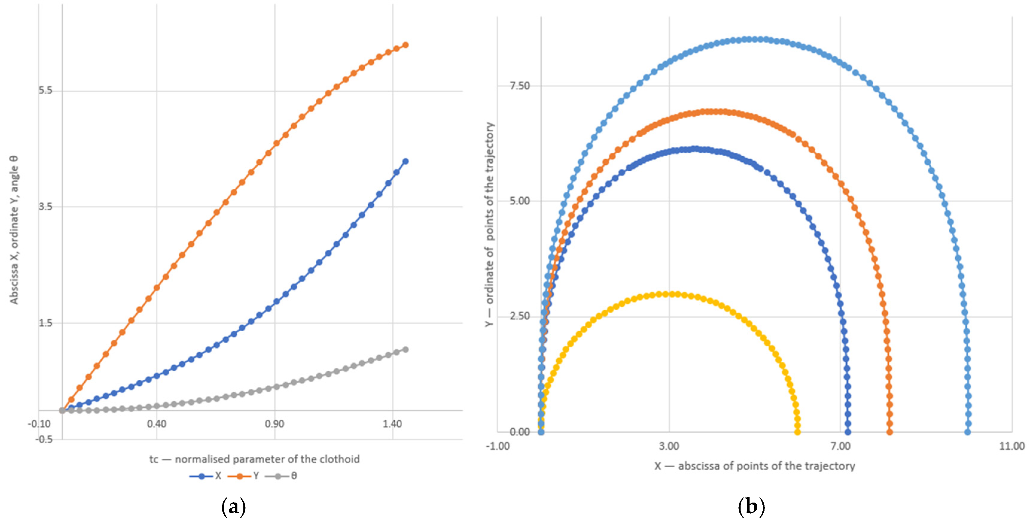
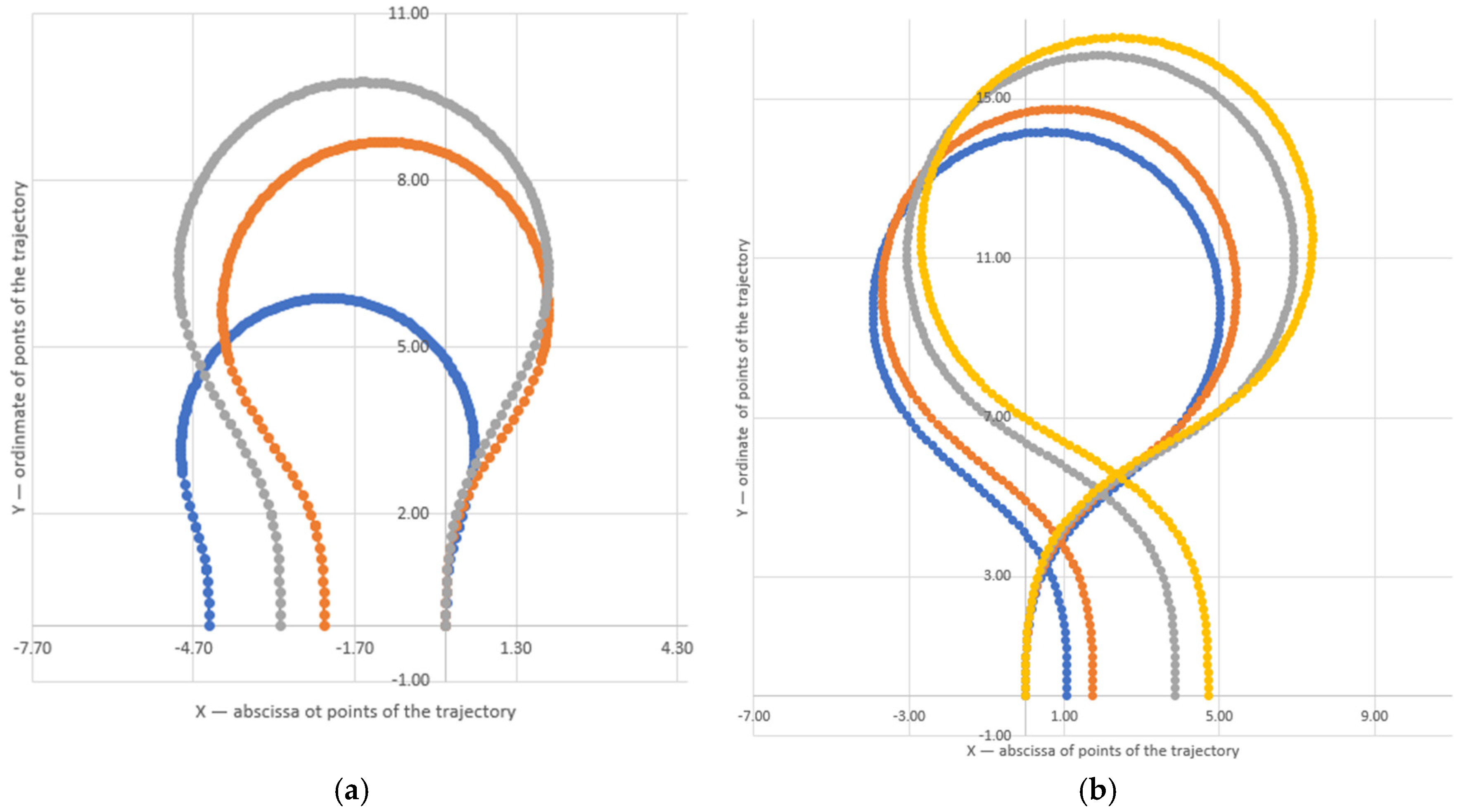
Of course, this also affects the points’ coordinates of this type of curve, for example, as is shown in Figure 4.

Figure 4. Relations for clothoids as part of the turn: (a) the abscissas—X, the ordinates—Y, and the angles of the tangents—θ, on the normalised parameter t; (b) its shape on the forward velocity Vc from 0—a semicircle, 0.84 m s⁻¹, 1.40 m s⁻¹, and 1.94 m s⁻¹ for the large curve. Starting point 0, 0. Steering rate ωc = 0.20 rad/s.

While the direction of movement changes in a relationship close to linear, the coordinates of the points are significantly affected, especially the ordinates (Figure 4a). The differences in curves—up to two times, when taking into account the influence of the velocity Vc—prove the usefulness of applying transition curves with clothoids for higher accuracy of the modelling (Figure 4b). Shown in Figure 4b are semicircle turns that consist of a forward right clothoid, arc, and backward right clothoid, with the exception of the smallest one. It is a semicircle stationary (pivot or zero-forward speed at the very beginning and at the very end) turn. The complexity of these relationships did not allow for obtaining statistically significant equations for them. Therefore, they remain to be obtained using numerical procedures.

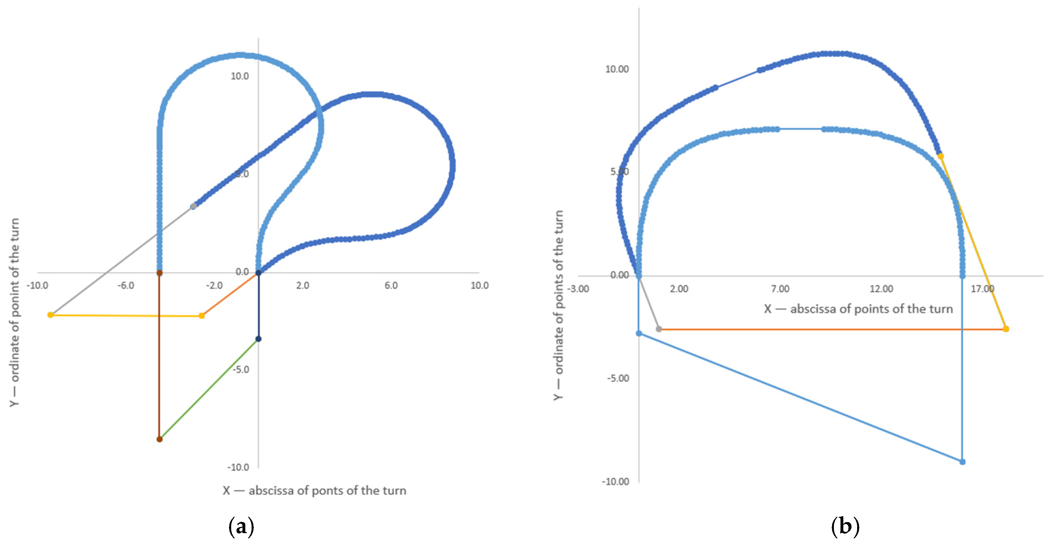
As expected, higher forward speed at the same steering rate results in longer turns. The explanation is the same as for semicircular turns. Higher speed leads to a later start for the arc movement. For this reason, in addition to the maximum steering angle, the distance between the entry and exit points for work passes can be adjusted by speed too. In the figure, there are two trajectories with the same distance: in (a), in blue colour, and in (b), in yellow colour. Of course, it is correct in such a case also to take into account the length and height of the turns. The height of the turns, determined by the greatest distance of the trajectory from the abscissa, also determines the minimum required width of the headland.

The greater possibilities for managing the parameters of such turns (mentioned above) also predetermine their wider use in agriculture. Of course, they cannot be replaced by semicircular turns, but they have other “competitors”.

Another type of turn, similar to those shown in Figure 5, is a P-turn (aka hook turn). Its basic characteristics are not much different from those of a light bulb and eight-formed turns. At the same time, motion in a straight line, if it is before the point of entry for work in the main area, allows for easily correcting any inaccuracies in guiding the tractor or self-propelled machine. This makes this turn accessible even to less experienced drivers.

Figure 5. Impact of forward speed on shape and dimensions of (a) light bulb turns and (b) eight-shaped turns. Starting points 0, 0. Forward speed in (a): 0.84 m s⁻¹, 1.40 m s⁻¹, 1, 95; in (b): 0.84 m s⁻¹, 1.40 m s⁻¹, 1, 95, 2.50 m s⁻¹. Higher forward speed = larger turns. Steering rate ωc = 0.20 rad/s.

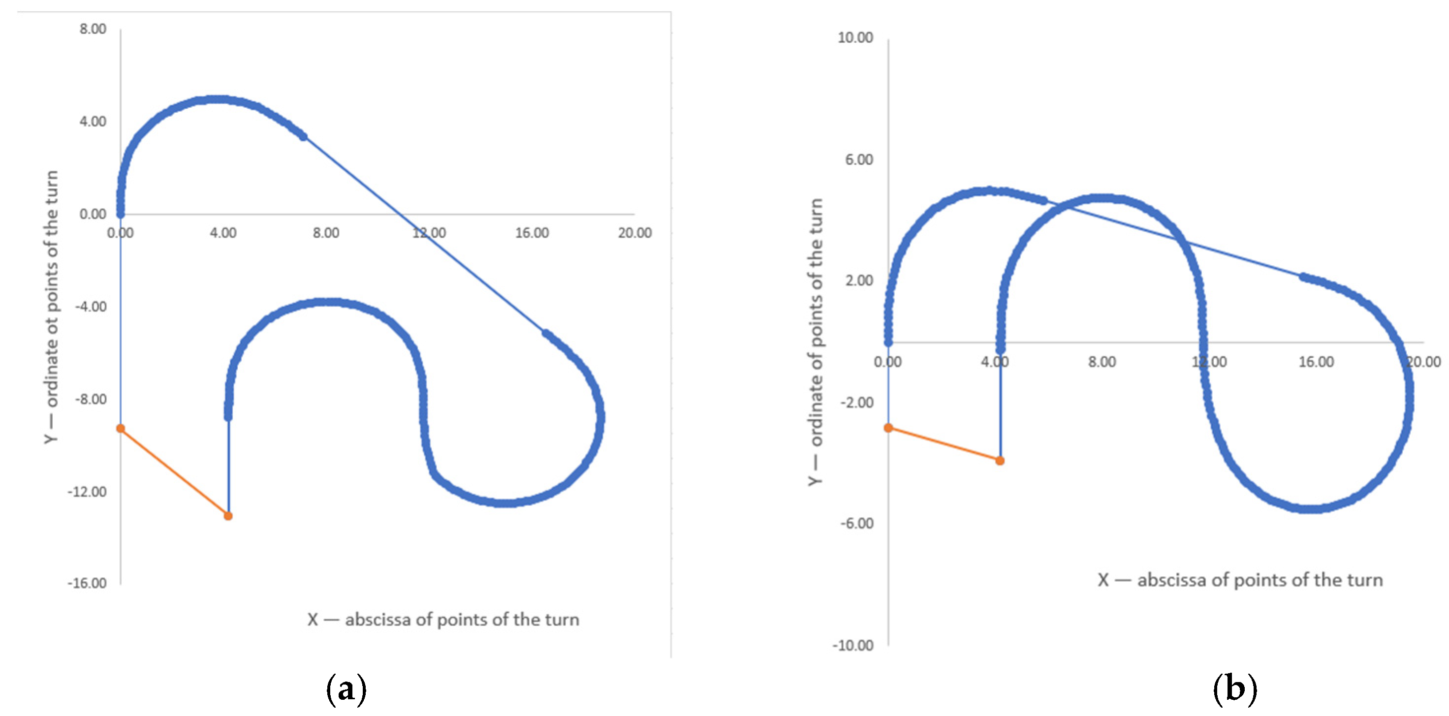
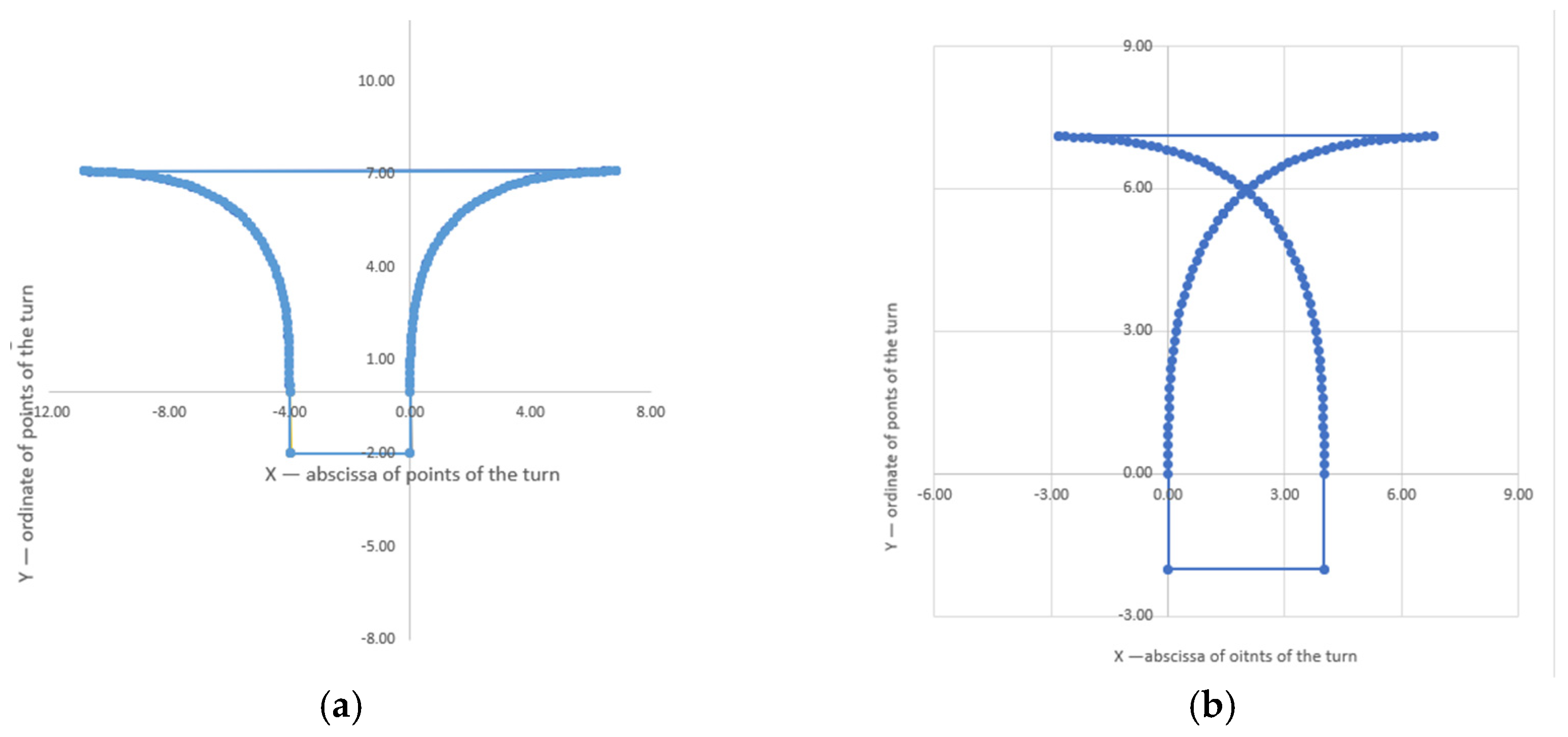
Such a turn is shown in Figure 6a in motion not perpendicular to the field boundaries conditionally to the north. The calculation of the height of this turn can be facilitated if the trajectory is simply translated so that the entry and exit points become parallel to the abscissa in the same figure.

Figure 6. Models of P-turn (a) and U-turn (b) with their rotated images when working passes are not perpendicular to the field boundaries. The red lines are parallel to the field boundaries.

The turns considered so far are related to the shuttle field pattern, aka a continuous alternation field pattern. Clarification is needed, as there are also other interpretations of these movements in the field. The authors assume that this refers to travel in which equipment moves back and forth across the field and where each pass is adjacent to the previous one. This field pattern with a light bulb turn, eight-formed turn, and R-turn is suitable for field operations such as sowing, spraying, and fertilising row crops. It makes it easier to guide the machines even in the absence of GPS navigation tools.

For a straight alternation field pattern (aggregates move also back and forth but skip one or more neighbouring tracks before turning) the U-turn is better (Figure 6b). If it is symmetric, it can show two symmetric left parts of the P-turn connected by a straight line. The last one makes it easier to have a necessary distance between the exit and entry points in the main field area by extending or shortening this line. At the same time, it needs wider turns (i.e., U-turns), planning, or a GPS for skips. That is why it is better for precision tasks like planting with autosteer.

The turns, shown in Figure 7, sometimes are good when an agricultural unit is traveling in the main field area in a direction not perpendicular to the field boundaries. In such cases, the length of the straight-line movement increases after exiting the main field and before entering it. Moreover, the double-cultivated area in the headland and the width of the headland are increasing. Using turns, as shown in Figure 4, can reduce the width of the headland and, respectfully, the area of the headlands, cultivated in a different way as the main field area. This happens if those used in other cases, like light bulb turns, eight-formed turns, or P-turns, are replaced by this, as mentioned above. However, it can be seen that such turns are quite complicated, especially in the absence of GPS navigation. In such cases, the part of P-turns in these turns can also be replaced with some of the previously discussed turns except for U-turns.

Figure 7. P-turns with side exit: (a) with a large deviation of the direction of the work pass relative to the field boundaries and (b) with a small one.

A special type of manoeuvre is the fishtail turn. Compared to the U-turn, the length of its straight segment can besignificantly shorter. Usually, in extended turns, three or more working passes are skipped. In fishtail turns, the field patterns may be continuous alternation (shuttle) or straight alternation with one, two, or more skipped passes. As a rule, three or more strokes are not preferred, since the time for the manoeuvre is significantly extended. This extension is a consequence of the necessary gear shifting and possible deceleration and acceleration. Such a fishtail turn can often be performed in two ways (Figure 8). Naturally, in such a case of shorter working width of the agricultural unit, the manoeuvre with a short length would be preferred (Figure 8b). The different scale of the figures requires that the comparison be made with particular attention to the numbers on the abscissa.

Figure 8. Fishtail turns with backward (reverse) travel and equal distance between the “run-out” and “run-in” points for the working field area: (a) with a long straight-line reverse travel; (b) with a short straight-line reverse travel.

The preceding simulations and kinematic analyses have demonstrated the significant impact of forward speed, steering rate, and the use of clothoid-based transition curves on the shape, dimensions, and spatial characteristics of various headland turns, including semicircular, light bulb, eight-shaped, P-turn, and U-turn trajectories. The results highlighted how these parameters affect not only the turning path and entry–exit alignment relative to field boundaries but also the minimum required width of headlands and the efficiency of shuttle or straight alternation field patterns. In the subsequent field experiments, reversible manoeuvres with backward motion were included to replicate realistic operational conditions and to assess their effect on the turning dynamics. While the simulations provide a detailed understanding of the geometric and kinematic properties of these manoeuvres, practical verification is required to evaluate their dynamic performance under real field conditions.

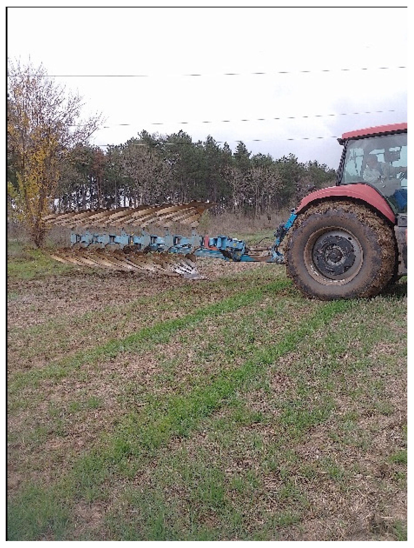
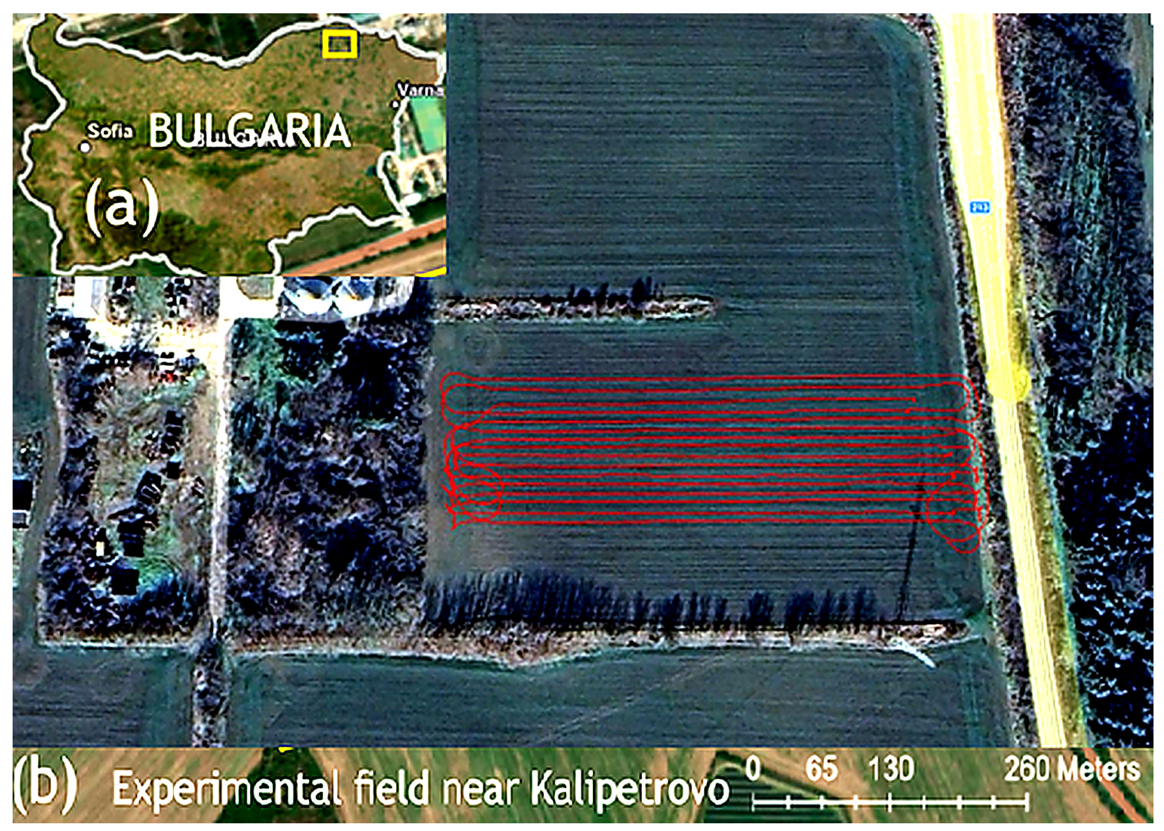
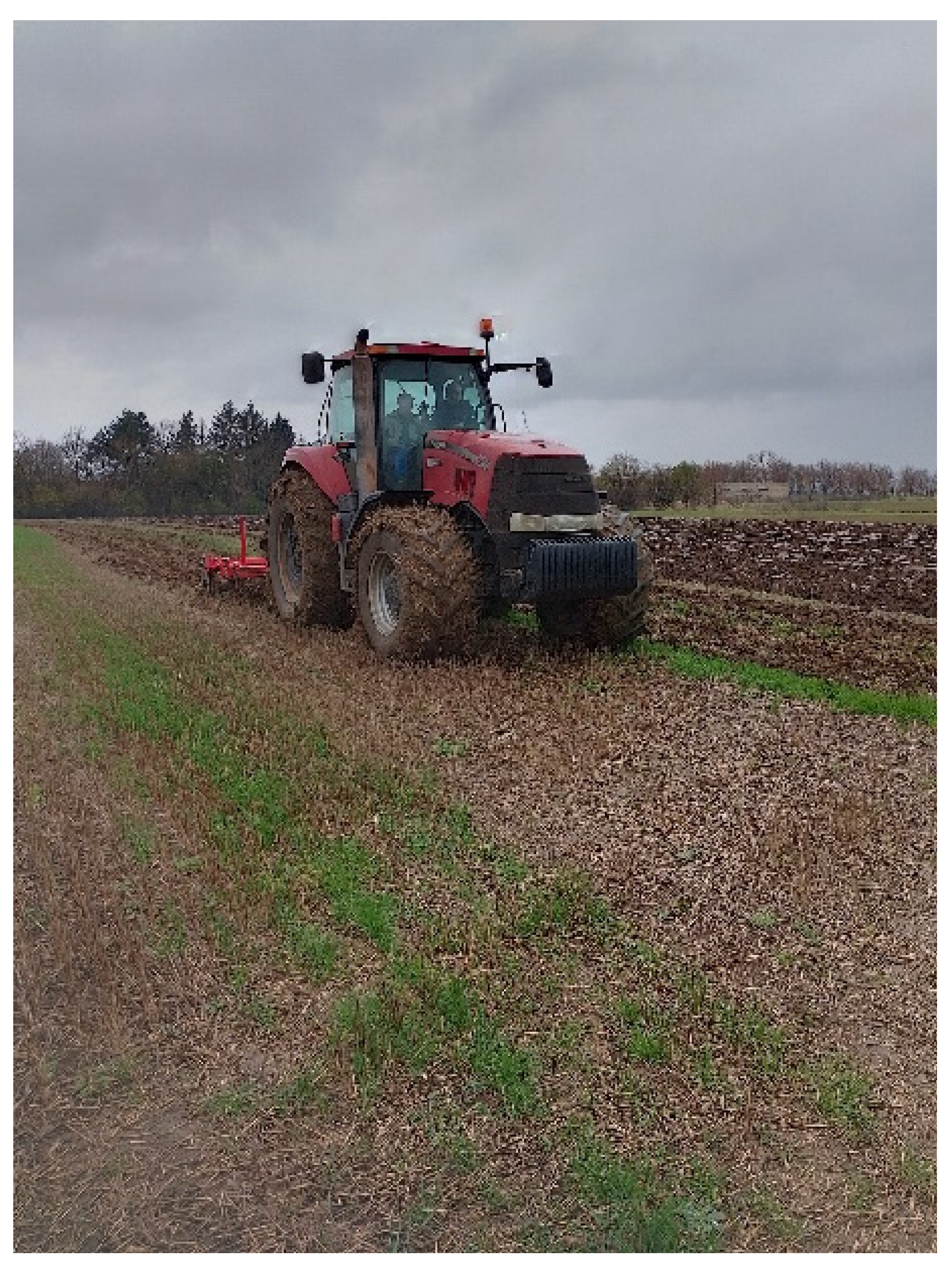
To analyse the characteristics of the investigated turning manoeuvres and to optimise the operational cycle, field experiments were conducted at the experimental site of the “Zlatno Zarno” cooperative. Two fundamentally different headland turning strategies were evaluated.

During ploughing operations, a continuous pear-shaped headland turn was applied, characterised by uninterrupted forward motion and a relatively large turning radius. In contrast, during subsoiling operations, a reversible turning manoeuvre involving a reverse motion segment was performed.

These turning strategies resulted in distinct velocity profiles and trajectory lengths, which are key parameters for assessing the operational productivity and energy consumption of the field operations. The quantitative differences in manoeuvre dynamics provide critical input for optimising both work cycle efficiency and energy management in mechanised tillage.

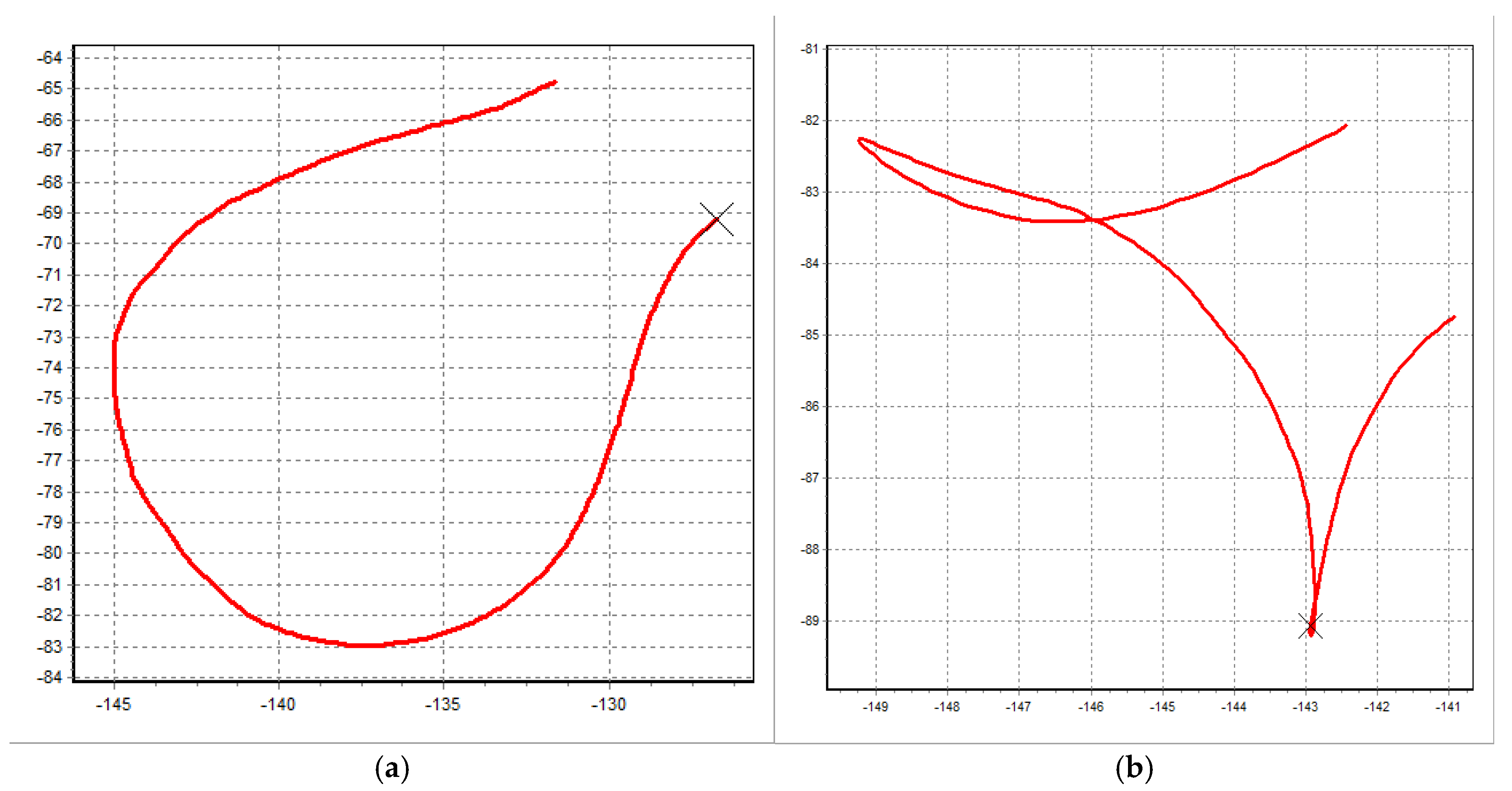
Figure 9 presents the actual movement trajectories of the two headland turning strategies, recorded using a GPS receiver. To assess the manoeuvring characteristics of the machine–tractor unit under different technological operations, two specific movement models were analysed.

Figure 9. GPS-recorded turning trajectories from field experiments represented via local trajectory mapping: (a) ploughing operations with a continuous pear-shaped headland turn and (b) subsoiling operations with a reversible turning manoeuvre.

Figure 9a illustrates the trajectory during ploughing operations, where a continuous pear-shaped headland turn is applied, characterised by uninterrupted forward motion and a smooth change in direction. Figure 9b shows the trajectory during subsoiling operations, performed using a reversible turning manoeuvre that involves two complete stops of the unit to change direction.

The differences in trajectory geometry and manoeuvring dynamics between these two approaches are critical for determining the total duration of idle strokes and the overall efficiency of the work cycle.

To quantitatively assess the accuracy of the developed model, the simulated trajectory coordinates were directly compared with the experimentally recorded GPS coordinates using root mean square error (RMSE) analysis. The RMSE values were calculated separately for longitude and latitude coordinates, as well as for the overall spatial trajectory deviation.

Table 1 summarises the statistical comparison between the theoretical model and the experimental GPS data.

Table 1. Regression-based statistical comparison of simulated and GPS trajectories.

Model Summary
Model	R	R Square	Adjusted R Square	Std. Error of the Estimate
Longitude, m	0.470	0.221	0.217	0.0412386
Latitude, m	0.616	0.379	0.377	0.0929374

The main indicator of the model’s accuracy is the root mean square error (RMSE), presented in the “Std. Error of the Estimate” column.

The calculated RMSE values were 0.041 m for longitude and 0.093 m for latitude, indicating a high level of spatial agreement between the simulated and observed machine trajectories. These low error values demonstrate that the developed model provides sufficient practical accuracy for simulating agricultural machinery manoeuvres at field headlands.

Additionally, the coefficient of determination (R²) values, together with the statistical significance level (p < 0.001), indicate a moderate to strong correspondence between the modelled and measured coordinates, further supporting the reliability of the proposed simulation framework.

The achieved accuracy (RMSE < 0.1 m) can be attributed to the controlled experimental conditions and the relatively constant machine operating speed, which reduced dynamic disturbances and GPS signal noise during trajectory recording.

The obtained correlation coefficients indicate moderate agreement between the simulated model and the GPS-measured trajectories, which is expected given the inherent noise and multipath effects in GNSS-based field measurements, as well as the dynamic nature of agricultural machinery operation. Therefore, model performance should be primarily assessed using spatial error metrics (e.g., RMSE), which provide a more direct and reliable measure of positional accuracy and confirm the practical validity of the proposed approach.

Table 2 and Table 3 present detailed descriptive statistics for the operational speed and the turning path length, respectively. The reported results include not only the mean values (Mean) and standard deviations (Std. Deviation), but also distribution shape indicators (Skewness and Kurtosis), as well as the range and 95% Confidence Intervals (CIs).

Table 2. Descriptive statistics for turning speed (km h⁻¹) according to manoeuvre type.

Type of Operation	Descriptives		Statistic	Std. Error
Ploughing	Mean		5.4835	0.05300
	95% Confidence Interval for Mean	Lower Bound	5.3726
		Upper Bound	5.5944
	5% Trimmed Mean		5.4672
	Median		5.4200
	Variance		0.056
	Std. Deviation		0.23703
	Minimum		5.14
	Maximum		6.12
	Range		0.98
	Interquartile Range		0.37
	Skewness		1.078	0.512
	Kurtosis		1.258	0.992
Subsoiling	Mean		3.5745	0.09388
	95% Confidence Interval for Mean	Lower Bound	3.3780
		Upper Bound	3.7710
	5% Trimmed Mean		3.5761
	Median		3.6350
	Variance		0.176
	Std. Deviation		0.41983
	Minimum		2.86
	Maximum		4.26
	Range		1.40
	Interquartile Range		0.63
	Skewness		−0.203	0.512
	Kurtosis		−0.747	0.992

Table 3. Descriptive statistics for turning path length (m) according to manoeuvre type.

Type of Operation	Descriptives		Statistic	Std. Error
Ploughing	Mean		44.3020	0.95585
	95% Confidence Interval for Mean	Lower Bound	42.3014
		Upper Bound	46.3026
	5% Trimmed Mean		44.3733
	Median		45.3000
	Variance		18.273
	Std. Deviation		4.27469
	Minimum		38.17
	Maximum		49.15
	Range		10.98
	Interquartile Range		8.29
	Skewness		−0.330	0.512
	Kurtosis		−1.633	0.992
Subsoiling	Mean		22.1625	0.41066
	95% Confidence Interval for Mean	Lower Bound	21.3030
		Upper Bound	23.0220
	5% Trimmed Mean		22.1756
	Median		22.3100
	Variance		3.373
	Std. Deviation		1.83651
	Minimum		19.30
	Maximum		24.79
	Range		5.49
	Interquartile Range		3.65
	Skewness		−0.236	0.512
	Kurtosis		−1.322	0.992

The data are stratified according to the type of manoeuvre: pear-shaped headland turn and reversible turning manoeuvre. This comprehensive statistical characterisation enables a detailed comparison of the stability and efficiency of the two technological approaches and provides a solid basis for the subsequent comparative analysis.

The statistical evaluation of the performance indicators (Table 2 and Table 3) demonstrates a clear and systematic divergence in the operational behaviour of the two headland turning strategies, confirming that their efficiency is strongly condition dependent rather than universally applicable.

Under ploughing conditions (Table 2), the pear-shaped turn enables a significantly higher operational turning speed of 5.48 km h⁻¹, which is a direct consequence of its continuous forward motion and elimination of stopping phases. This uninterrupted kinematic behaviour not only increases productivity but also ensures a highly stable dynamic response, as reflected by the low speed variability (SD = 0.24). Such stability indicates minimal control effort and reduced mechanical stress on the transmission system, making this strategy particularly suitable for high-intensity operations where efficiency and motion continuity are critical design objectives.

In contrast, subsoiling operations (Table 3) reveal a fundamentally different performance regime. The reversible turning strategy reduces the average turning speed to 3.57 km h⁻¹ and introduces substantially higher variability (SD = 0.42), which is a direct consequence of discrete operational phases including stopping, reversing, and gear shifting. Although this results in reduced kinematic smoothness, it should not be interpreted as inefficiency in a global sense, since the same strategy achieves a nearly twofold reduction in trajectory length (22.16 m vs. 44.30 m), significantly improving spatial efficiency and reducing non-productive field boundary usage.

This trade-off between dynamic efficiency and spatial efficiency defines the core operational distinction between the two manoeuvres. The pear-shaped turn maximises productivity at the cost of increased spatial demand, whereas the reversible turn sacrifices kinematic smoothness in favour of minimising land loss and improving headland utilisation.

From a systems engineering perspective, these results strongly indicate that no single turning strategy is universally optimal. Instead, the optimal choice is strictly governed by field geometry and operational priorities: the pear-shaped turn is optimal in large, regular fields, where speed and continuity dominate performance requirements, while the reversible strategy becomes superior in constrained or irregular field geometries, where spatial efficiency and land preservation are dominant constraints.

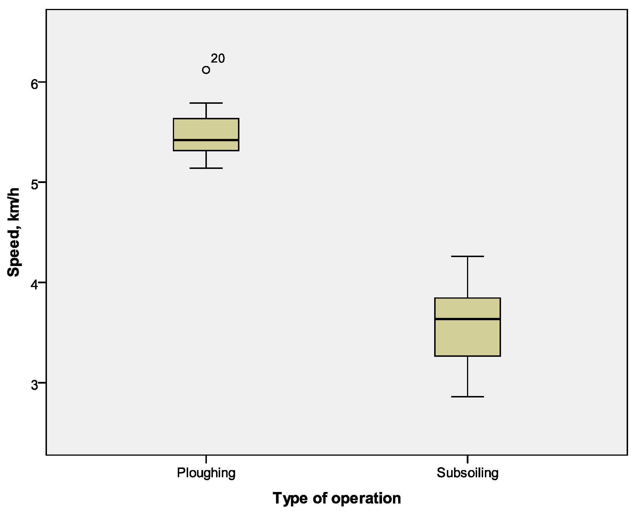
The skewness and kurtosis values further confirm that for ploughing, the turning speed data are more tightly concentrated around the mean, whereas for subsoiling, a more uniform distribution of turning speeds is observed across the entire range, reflecting the variable dynamics inherent to this operation. The graphical representation of turning speed using a Boxplot diagram (Figure 10) clearly illustrates the significant differences in the dynamic patterns of the two operations.

Figure 10. Variation of turning speed during ploughing and subsoiling operations.

The Boxplot for ploughing operations is positioned significantly higher along the speed axis, with the median turning speed concentrated around 5.42 km h⁻¹. In contrast, the Boxplot for subsoiling operations is shifted downward to the interval 3.20–3.90 km h⁻¹. The greater height of the subsoiling Boxplot reflects a larger interquartile range (IQR = 0.63) and a higher degree of variability associated with this manoeuvre.

For ploughing, a characteristic outlier (marked as 20) is observed, corresponding to a speed above 6.00 km h⁻¹. This confirms the presence of a single deviation beyond the typical operating range for this type of turn. Notably, the two Boxplots do not overlap, clearly indicating that the differences in turning speed between the two operations are statistically significant.

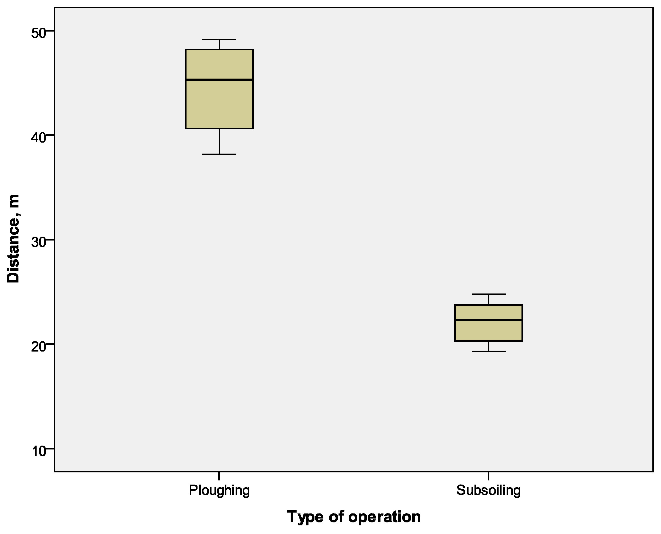
For a comprehensive characterisation of the two approaches, it is essential to compare not only the speed but also the geometric scale of the turns. Figure 11 presents a comparison of the turning path length for the two technological operations using a Boxplot diagram.

Figure 11. Turning path length during ploughing and subsoiling operations.

The graph in Figure 11 reveals a significant difference in the spatial parameters of the studied manoeuvres. While in a “pear” turn the median trajectory length is about 45.30 m, in a reverse turn with a backward manoeuvre it is reduced to nearly 22.31 m. It should be noted that despite the lower operating speed during deepening, this method allows the turn to be performed within significantly more compact limits. The lack of overlap between the two “boxes” and the whiskers on the diagram is a clear visual indicator that the two types of turns form two statistically different groups in terms of the distance travelled.

After the descriptive statistics and Boxplot analysis indicated observable differences in the mean values of the two groups, it was necessary to determine whether these differences are statistically significant or merely the result of random variation. To this end, an Independent Samples t-test was applied, comparing the mean values of the two independent groups (ploughing and subsoiling) with respect to the quantitative variables of turning speed and turning path length.

The primary objective of the test is to evaluate the null hypothesis (H₀), which states that no true difference exists between the two methods. A significance level (p-value) below the conventional threshold of 0.05 provides scientific evidence that the choice of technological approach (pear-shaped headland turn versus reversible turning manoeuvre) has a measurable impact on the operational performance of the machine–tractor unit. The test results, presented in Table 4, confirm the statistical significance of the differences in turning speed and turning path length between the two types of manoeuvres.

Table 4. Independent Samples test.

		Levene’s Test for Equality of Variances		t-Test for Equality of Means
		F	Sig.	t	df	Sig. (2-Tailed)	Mean Difference	Std. Error Difference	95% Confidence Interval of the Difference
									Lower	Upper
Speed, km/h	Equal variances assumed	6.946	0.012	17.708	38	0.000	1.90900	0.10781	1.69076	2.12724
	Equal variances not assumed			17.708	29.995	0.000	1.90900	0.10781	1.68883	2.12917
Distance, m	Equal variances assumed	33.962	0.000	21.281	38	0.000	22.13950	1.04033	20.03346	24.24554
	Equal variances not assumed			21.281	25.783	0.000	22.13950	1.04033	20.00019	24.27881

The results of the Independent Samples T-test strongly reject the null hypothesis. The values in the “Sig. (2-Tailed)” column for both indicators (turning speed and turning path length) are 0.000, indicating that the probability that the observed differences are due to chance is less than 0.1% (p < 0.001).

For turning speed, the calculated t-value of 17.708 demonstrates a substantial difference in favour of the pear-shaped headland turn, with an average speed difference of 1.91 km h⁻¹. Regarding turning path length, the t-value of 21.281 and an average difference of 22.14 m confirm that the pear-shaped turn is significantly longer than the reversible turning manoeuvre.

Furthermore, Levene’s Test for Equality of Variances shows a significance below 0.05, confirming that the two operations exhibit different variability. Overall, the statistical analysis provides robust evidence that the choice between the two types of turns results in fundamentally different performance indicators for the machine–tractor unit.

4. Discussion

In the present work, the transient processes of change in the direction of motion described by clothoids were shown to lead to a significant increase in both the length and height of headland turns compared to idealised instantaneous direction changes. This finding aligns with previous research emphasising the importance of accounting for realistic steering kinematics rather than simplistic geometric approximations. For example, Boryga [25] demonstrated that employing trigonometric transition curves in headland trajectory planning ensures smooth changes in curvature and steering angles, improving manoeuvre smoothness compared with traditional circular arc approximations. Similarly, He et al. [26] highlighted that dynamic path planning methods for unmanned agricultural vehicles can significantly reduce trajectory length and manoeuvre time, reinforcing the benefits of kinematic-aware modelling.

When compared with classical methods such as the tabulated equivalent turning radius [2], several limitations become apparent. The tabulated data cover a narrow range of implement sizes and lack information on specific turn types and steering dynamics, particularly for equipment with large working widths (e.g., sprayers and spreaders). Consequently, direct comparison with complex turn models, such as clothoid-based transitions, is challenging. Li et al. [27] further demonstrated that real-time trajectory planning using panoramic vision and sequential frame correlation enables agricultural vehicles to adapt to varying field conditions, reducing operational inefficiencies and confirming the shortcomings of static radius tables. Yang et al. [28] also showed that multi-objective adaptive path planning frameworks effectively optimise headland manoeuvres in dynamic field environments, further validating the importance of advanced kinematic modelling.

The application of modern machine learning methods, such as reinforced learning, shows the possibility and effectiveness of such approaches [9,29,30,31]. However, the last three suggested papers primarily focus on wireless communications and sensor applications, not on agricultural machinery trajectory planning or soil–implement interactions. While the proposed methodology is technically valuable, it does not fully align with the scope of our research, which focuses on field turns for agricultural machinery management, not fully autonomous manoeuvres.

The experimental results obtained in this study provide strong empirical support for these theoretical findings. As summarised in Table 1, Table 2 and Table 3 and illustrated in Figure 9, Figure 10 and Figure 11, the choice of manoeuvre substantially impacts operational performance. During ploughing, the pear-shaped headland turn allows for maintaining a significantly higher average turning speed (5.48 km h⁻¹) with greater stability, as indicated by the low interquartile range and standard deviation (Figure 10, Table 1). In contrast, the reversible turn with backward motion applied during subsoiling is associated with technological pauses, reducing the average speed to 3.57 km h⁻¹.

A clear trade-off between speed and spatial compactness is evident. Although slower, the reversible turn occupies on average half the distance (22.16 m) compared to the continuous pear-shaped trajectory (44.30 m) (Figure 11, Table 2), making it more suitable for operations in confined headlands or narrow field strips. The results of the Independent Samples T-test (Table 3) confirm with 100% confidence (p < 0.001) that these differences are not random but are a direct consequence of the geometry and kinematics of the two types of turns.

Previous studies have emphasised that headland traversal strategies significantly influence the total non-working distance travelled by agricultural machines, and algorithmic approaches can drastically reduce idle travel distances by optimising traversal sequences rather than relying on operator judgment or simplistic lookup tables. In particular, Bochtis and Vougioukas (2008) [12] framed field coverage as a graph traversal optimisation problem, demonstrating reductions in non-working distances of up to 50% through optimal routing. This finding aligns closely with our experimental observations: reversible manoeuvres, although slower, minimise spatial footprint and idle movement, whereas continuous pear-shaped turns maximise operational speed but require more space at the headland.

These findings underscore that for optimising the performance of machine–tractor units and considering specific field geometries, the proper selection of turn type is crucial. For long work passes, where maintaining high and consistent speed is prioritised, continuous trajectories such as the pear-shaped turn are more efficient for reducing manoeuvring time. Conversely, in fields with limited turning strips, reversible manoeuvres are preferred to minimise idle travel and optimise spatial usage, despite their lower dynamic speed.

Nevertheless, the limitations of the current modelling framework should be acknowledged. Processing large input datasets—characterised by numerous spreadsheet rows or columns—imposes computational challenges, particularly when high-resolution turn profiles are required. Visualisation of model outputs currently requires manual specification of axis scales and plot dimensions, which can become cumbersome for extensive comparative studies or real-time systems.

Future research directions include automating the computational workflow, integrating the clothoid-based model with autonomous navigation stacks, and exploring machine learning approaches to adapt turn parameters based on historical field performance. Such developments would further enhance efficiency beyond deterministic models and bridge the gap between theoretical trajectory planning and field implementation.

In conclusion, while traditional tables of equivalent radii may offer simplicity, they are insufficient for capturing the nuanced steering behaviour of modern agricultural machinery. The clothoid-based modelling procedure, complemented by real-world experimental verification and supported by advanced trajectory planning frameworks [25,26,27,28], provides improved accuracy, flexibility, and relevance for precision field operations. The experimental evidence clearly demonstrates that turn type selection significantly affects operational speed, spatial efficiency, and overall performance, underscoring the importance of integrating both kinematic modelling and field testing in the optimisation of headland manoeuvres.

5. Conclusions

Modelling headland manoeuvres using transition curves based on clothoids effectively captures the significant influence of forward speed and steering velocity on the geometry and dynamics of turns. Incorporating the tangent angle (direction of motion) in the description and visualisation of trajectories within a spreadsheet environment provides a practical and accessible tool for analysing complex headland turns, enabling both simulation and visual verification.

The experimental verification conducted in the field demonstrates that the choice of turn type has a substantial impact on operational performance. Pear-shaped continuous turns, as observed during ploughing, allow for higher average speeds (5.48 km h⁻¹) and greater stability, with low variability in speed and path length. Conversely, reversible turns with backward manoeuvres, applied during subsoiling, result in lower average speeds (3.57 km h⁻¹) but occupy significantly less space at the headland, reducing the distance travelled during the turn by approximately 50% (22.16 m vs. 44.30 m for pear-shaped turns).

Statistical analysis using the Independent Samples T-test confirmed with high significance (p < 0.001) that these differences are not random but directly result from the geometry and kinematics of the two types of manoeuvres. The results clearly illustrate a trade-off between speed and spatial compactness: continuous turns maximise operational velocity and minimise manoeuvring time on long field passes, whereas reversible turns optimise space utilisation in constrained headlands or narrow field strips, thereby minimising non-productive travel.

The combination of kinematic modelling and real-world experiments highlights the importance of selecting the appropriate headland turning strategy based on field geometry and operational objectives. The proposed clothoid-based modelling procedure offers improved accuracy for estimating turn length and height, which is crucial for optimising field efficiency, reducing fuel consumption, and minimising machine wear. Moreover, integrating simulation results with statistical verification strengthens the reliability of operational recommendations.

Future research should focus on further extending the modelling framework to support a broader range of headland manoeuvres and operational conditions beyond those examined in the current simulations. Such developments would provide a more comprehensive tool for evaluating headland strategies, particularly in confined fields where manoeuvring space is limited. Additional directions include the development of automated workflow tools, integration with autonomous navigation systems, and adaptation of turn parameters through machine learning algorithms based on historical field performance.