Article

Predicting Venue Popularity Using Crowd-Sourced and Passive Sensor Data

Chair of Transportation Systems Engineering, Department of Civil, Geo and Environmental Engineering, Technical University of Munich, 80333 Munich, Germany
*
Author to whom correspondence should be addressed.
Smart Cities 2020, 3(3), 818-841; https://doi.org/10.3390/smartcities3030042
Submission received: 21 June 2020 / Revised: 30 July 2020 / Accepted: 4 August 2020 / Published: 6 August 2020
(This article belongs to the Special Issue Feature Papers for Smart Cities)

Abstract

:
Efficient and reliable mobility pattern identification is essential for transport planning research. In order to infer mobility patterns, however, a large amount of spatiotemporal data is needed, which is not always available. Hence, location-based social networks (LBSNs) have received considerable attention as a potential data provider. The aim of this study is to investigate the possibility of using several different auxiliary information sources for venue popularity modeling and provide an alternative venue popularity measuring approach. Initially, data from widely used services, such as Google Maps, Yelp and OpenStreetMap (OSM), are used to model venue popularity. To estimate hourly venue occupancy, two different classes of model are used, including linear regression with lasso regularization and gradient boosted regression (GBR). The predictions are made based on venue-related parameters (e.g., rating, comments) and locational properties (e.g., stores, hotels, attractions). Results show that the prediction can be improved using GBR with a logarithmic transformation of the dependent variables. To investigate the quality of social media-based models by obtaining WiFi-based ground truth data, a microcontroller setup is developed to measure the actual number of people attending venues using WiFi presence detection, demonstrating that the similarity between the results of WiFi data collection and Google “Popular Times” is relatively promising.

1. Introduction

The popularization of social media due to recent progress in broadband networks and mobile device technology has brought about enhanced interest in location-based services for the travel demand modeling domain and transport planning. Location-based services and their integration within social media (e.g., Facebook, Twitter, Foursquare) have contributed to the advent of “location-based social networking” (LBSN), providing accurate location and trip purposes to connected users of the same platform. Such data can potentially deal with the drawbacks of conventional data sources used for mobility pattern inference (e.g., travel surveys and GPS or phone signal traces), such as cost of collection, privacy issues and missing data [1,2]. The major advantage of LBSN in travel demand modeling is that each geographical trace is coupled with its trip purpose, i.e., a “check-in” at a specific bar indicates a recreational visit, while a trace at a university mostly reflects an educational activity. The vast majority of studies on the exploitation of LBSN have used Twitter and Foursquare, e.g., [1,3,4]. However, traces are often accompanied by a systematic temporal error and there is a temporal and spatial bias in the appearance of digital traces for venue visits [5].
Scellato et al. [6] carried out comprehensive research to investigate the spatial characteristics of the social networks arising among users of different popular LBSNs: Brightkite, Foursquare and Gowalla. The results showed that LBSNs can provide universal spatial features across them, irrespective of the service, its number of users or the adopted sampling approach. Muhammad et al. [7] have attempted to explore the LBSN data to analyze gender-based check-in behavior during weekdays and weekends by focusing on the most popular Chinese local social network site, Sina Weibo, with their research area defined as Guangzhou, China. The findings indicated that female users are more inclined to use Weibo compared to male users during the weekdays. Nevertheless, both male and female users follow roughly the same check-in trend during the weekend.
Google “Popular Times” [8] provide information on when a venue is mostly visited, live waiting time, as well as average visit duration, based on aggregated and undisclosed data from users who have opted to share their geotrace using their mobile devices. Such information could potentially improve real-time demand estimation for transportation planning applications, thus enhancing traffic management around hotspots. Nevertheless, to date, “Popular Times” have not yet been widely utilized for transport planning purposes but rather for high-level descriptive impacts on traffic [9].
Venue popularity modeling is a trending topic in the literature which has recently attracted considerable attention. The aim of this paper is to (i) exploit several data sources including Yelp, Google Maps, OpenStreetMap (OSM), as well as population and workplace information for venue popularity modeling and (ii) overcome the drawbacks of aggregated geo-locating data by providing an alternative measuring methodology based on cost-efficient WiFi microcontrollers.
The potential of using geospatial information to the advantage of users was highlighted by Meeks and Dasgupta [10], evaluating the use of information for decision-makers and users of systems. Geospatial data have become widely available through open-source platforms (e.g., OSM) and social media and have been used in a wide variety of venue-related research since then.
For example, Kisilevich et al. [11] used OSM data for predicting hotel room prices and hotel values. Based on information on location, places of interest (museums, landmarks, restaurants and bars in the vicinity etc.) and hotel and business characteristics, the authors developed an easily extendable decision support tool for hotel brokers and demonstrated that the most influential parameter for determining the value of a hotel room was the proximity of the hotel to the city center. On the same principle, Wang et al. [12] investigated the effect of Foursquare “check-ins” and Yelp reviews and price ranges on venue success and failure. These two location and social services were combined with business features (e.g., number of direct competitors in the vicinity, number of special promotions of business and competitors) in order to identify business failures of restaurants in New York. The authors used a plethora of machine learning approaches, such as neural networks (NNs), k-nearest neighbors (k-NN) and binary logit, and concluded that the odds of failure of a restaurant are closely linked with the number of check-ins at that particular restaurant and the number of check-ins in nearby places of interest.
Geospatial information and LSBN data are often used in shared mobility studies [5,13,14] and mainly in estimating demands, flows or travel behavior purposes [15,16,17,18,19]. However, there remains a paucity of evidence on the utilization of LBSN for venue popularity and recommendation.
With regard to venue popularity, Wang et al. [12] analyzed the influence of Foursquare check-ins on business failure. Several features from Yelp and Foursquare were studied, including business features (e.g., price range, rating, the number of direct competitors within a certain area, the number of special promotions of business and competitors within a certain area) and check-in data (e.g., average daily check-ins of business and neighbors, growth rate). They showed that the increase in a restaurant’s average daily check-in rate and the number of days on which the growth rate has increased are associated with a significant decrease in the odds of failure. They also found that rating was positively correlated with failure, which can be attributed to higher business costs and therefore lower profit margins. Interaction between rating and the number of competitors within an area was also significant. Li et al. [4] explored three venue characteristics: venue profile information, venue category and venue age. The main findings indicated that the popularity of older venues is higher than newer ones (with some exceptions); the most mentioned venues belong to the food category; the transport category (e.g., airports) has the highest amount of check-ins. More recently, Yang and Durarte [20] investigated the influence of Foursquare check-ins on the popularity of a venue, as well as the spatiotemporal relationship between venues in Barcelona, Spain, and highlighted the importance of using WiFi sensors to identify the density of venue popularity. Moreover, with point of interest (POI) data as an approximation of places in cities, Liu et al. [21] developed representation learning models to explore place niche patterns, generating two main outputs: distributed representations for place niche by POI category (e.g., restaurant, museum, park) in a latent vector space and conditional probabilities of POI appearance of each place type in the proximity of a focal POI. With case studies using Yelp data for four U.S. cities, they showed that some POI categories have more unique surroundings than others. Van Weerdenburg et al. [22] also proposed a method to extract leisure activity potentials from web data on urban space using semantic topic models. Finally, based on geolocated webtexts and place tags, three supervised multi-label machine learning strategies were tested to estimate whether a given type of leisure activity is afforded or not.
On the other hand, research on venue recommendation systems is usually concerned with developing prediction mechanisms of venue attractiveness according to user’s preferences, as well as time and location restrictions [23,24]. Noulas et al. [25] suggested several mobility features, e.g., popularity (the total number of venue check-ins), geographic distance, rank distance, activity and place transitions for venue prediction, and outlined that popularity and distance are the most important factors for venue decision.
In the domains of venue popularity and recommendation, data collection is usually carried out with video recognition systems, as well as wireless sensing such as WiFi and Bluetooth. For example, Abrishami et al. [26] collected data with WiFi monitoring devices in over 100 places in the USA and used it to predict actual foot traffic for the next 168 h (week). Data from past traffic observations were used to predict future states. Bluetooth was utilized by Yoshimura et al. [27] to analyze museum visitors’ behavioral patterns. However, the main drawback of this approach was the detection of only mobile devices with Bluetooth turned on, which could lead to possible biases in the results, as only 8.2% of visitors had activated this function. In the paper of Nunes et al. [28], the authors used WiFi tracking technology to analyze tourist mobility patterns. In this research, authors had ground truth data from tourist authorities and were able to correlate it with sensor data and, for certain places, with Google “Popular Times”. Their results showed that there is a strong correlation between ground truth and sensor data, as well as quite a high correlation between sensor data and Google “Popular Times”.
Understanding human check-in behavior within a city and crowd dynamics in urban environments using social media check-ins is essential for several applications, such as urban planning, activity analysis, traffic prediction and location-based services [29]. Up until now, researchers have mainly developed travel demand models based on traditional travel surveys, which are expensive and can lead to issues such as short survey duration, high respondent burden and small sampling rates. By contrast, emerging data collection methods can support researchers to leverage state-of-the-art machine learning methods with a large amount of mobility data for extracting daily check-in behavior and latent mobility patterns. The main aim of this research is to investigate the quality of location-based social media data, especially Google “Popular Times” data, by obtaining WiFi-based ground truth data, Indeed, the capability of Google “Popular Times” data in modeling venue popularity is quantified by comparing them with WiFi device presence detection. To achieve this goal, this paper contains two main analyses: firstly, using geospatial properties of venues to predict their popularity, represented by Google “Popular Times” data; secondly, quantifying whether Google “Popular Times” data are a good measure of venue popularity by leveraging data collected from WiFi devices.
In summary, LBSNs have attracted significant attention in mobility studies and venue-related research. What remains unclear, however, is how to use Google “Popular Times” with WiFi sensors to identify venue popularity and recommendation. This combination forms the motivation for the present research and will be investigated in order to overcome the aforementioned limitations.
This research is designed to evaluate the possibility of using several information sources, including Google “Popular Times” and venue catalogues such as Yelp, as well as OpenStreetMap (OSM) data, for estimating venue popularity. Initially, data from the above-mentioned data sources are used to model venue popularity. In order to estimate hourly venue occupancy, two different classes of models are employed, including linear regression with lasso regularization and gradient boosted regression (GBR). Since Google “Popular Times” data can merely represent relative venue attendance, a cost-effective WiFi microcontroller setup is developed and tested to measure the actual number of people attending a particular venue using WiFi device presence detection. Finally, our real-world tests in Munich, Germany, demonstrate a promising similarity between the results of WiFi data collection and Google “Popular Times”.
The remainder of this paper is organized as follows: Section 2 presents the methodology, followed by Section 3 encompassing the modeling process. Section 4 includes a discussion of venue popularity measuring. Finally, Section 5 draws conclusions and provides insights for further research.

2. Methodology

As Figure 1 shows, the present research was comprised of two main parts, including venue popularity modeling and venue popularity measuring, which are described in the forthcoming sections. Nowadays, several novel sources of information with an unprecedented volume, termed ‘‘big data”, are being leveraged to supplement or substitute traditional survey data to extend human travel behavior research. This can provide a tremendous opportunity to revolutionize the transportation field due to the considerable data volume collected on the real-time location and dynamics of users. Accordingly, in the first part of the study, we used OSM data and data from Yelp and Google Places to generate independent variables and to predict hourly relative popularity indices obtained from Google’s “Popular Times” data, based on gradient boosted regression and linear regression with lasso feature selection. In the second part of the paper, we compare the “Popular Times” index data with WiFi-based crowding measurements obtained in a handful of venues.

2.1. Research Area

Real-world tests were conducted in Munich, which is the capital and the most populated city in the German state of Bavaria, with a population of around 1.5 million (https://www.muenchen.de/rathaus/Stadtinfos/Statistik/Bev-lkerung.html), and the third largest city in Germany. Regarding the study area, we considered the central point of activities in the city (with the majority of them related to food), located quite close to Marienplatz (https://www.muenchen.de/sehenswuerdigkeiten/orte/120347.html), Karlsplatz (Stachus) (https://www.muenchen.de/sehenswuerdigkeiten/orte/120328.html) and Hauptbahnhof (https://en.wikipedia.org/wiki/M%C3%BCnchen_Hauptbahnhof) (main train station), which are also in the city center and historical center.

2.2. Data Sources

As can be seen in Table 1, several different data sources, accessed in August 2018, were used in this study, including Google Maps, Yelp, OpenStreetMap (OSM), Google application programming interface (API) and government data on workplaces and population.
Yelp: At the first step of data collection, basic data were collected based on available venues and the Yelp website (see Figure 2). Here, it was possible to extract venue name, price level, rating, number of reviews and venue tags and address. Extraction was made based on venue type (for example, restaurants).
Google Maps: Based on names and addresses from yelp.com, additional information was extracted from Google Maps (see Figure 3 and Figure 4), e.g., price level (available at few venues), rating, number of reviews, “Popular Times” and opening hours.
Google location API: Geocoding (obtaining latitude and longitude) of venues based on name and address (this is also possible with OSM; however, results could be relatively inaccurate) was necessary for the next project step (referencing of objects). Geocoding was conducted with a simple request to the Google server. It was also necessary to obtain a free developer API key to make these requests. The main drawback of Google location API is the limitation of requests for a free account.
Referencing of objects: To assign spatial information to the venues collected in previous steps, several procedures were implemented. OSM data were loaded with the osmread library (https://github.com/dezhin/osmread) to obtain only ways and nodes related to Munich area. Then, the road graph was loaded with the osmnx library (https://github.com/gboeing/osmnx) (via the OSM API) and projected on a map. Venue coordinates, loaded in the previous step, were used to obtain central points. Then, the road graph was used to obtain all roads within the venue’s surrounding area. Two distances of influence were tested, 400 and 800 m, with the former being quite common among the literature, e.g., see review in [13]. Road endpoints were used to construct convex hulls. All nodes, ways, population grid cells and sum of workplace values from buildings and intersecting/within convex hulls were added to appropriate variables. Note that, since population data were available in the form of grid cells with an adequate spatial resolution, no disaggregation steps were needed. However, workplace data are relatively aggregate; therefore, a disaggregation algorithm was used to distribute workplaces among Munich administrative areas.

2.3. Data Structure

Variables were defined based on tag names from Yelp, classes and class groups of OSM and venue type. A number of variables such as rating and reviews were combined, and some others such as latitude and longitude were converted to proper projections. Regarding working hours, current hour and two hours in each direction were used in order to limit collinearity (see Table 2). All Google “Popular Times” values were assigned to dependent variables.
It should be noted that all the experiments in this research were implemented using the Python programming language and several Python libraries (Table 3), as well as others included in Anaconda (https://www.anaconda.com/download/) distribution.

3. Modeling

Two different classes of prediction model, including multiple linear regression with lasso and gradient boosted regression (GBR), were tested. Moreover, the performance of models with and without transformation was evaluated. Each model group tested comprised 168 dependent variables (i.e., the number of hours in a week), place parameters (e.g., rating, the number of related comments, type of service provided) and locational properties (e.g., the number of stores, hotels, attractions). Overall, we saw that GBR (Table 4) could provide a significantly better fit for the training set in comparison with linear regression (Table 5). Moreover, Figure 5 and Figure 6 give information regarding Box–Cox parameter selection for GBR and multiple linear regression models, respectively. The most important features for all GBR models are shown in Figure 7, Figure 8 and Figure 9. The number of features with the sum of importance of higher than the threshold (0.6 was used here to limit their number to a manageable level) was decreased for transformed models, declining from 51 to 35 with logarithm transformation (Figure 8) and from 51 to 34 with Box–Cox transformation (Figure 9). Some venue features, such as “burgers”, also achieved significant importance, especially at certain hours, e.g., early in the morning. This might be due to an activity transition from clubs or bars to fast-food venues, which may serve burgers and may be opened at this time. The relatively small significance of spatial features may arise from the fact that a large number of venues with available popularity values are located close to each other. Nonetheless, “nodes_osm_accomodation” (the variable including hotels, hostels and short term rented apartments) was quite significant.
A cross-validation method with 10 folds was used for each output (for number of trees selection and separately for cross-validation). To reduce computational complexity, a relatively high learning rate of 0.01 was used. After running a GBR model, residuals were tested for several problems (see Figure A1 and Figure A2 in Appendix A). Since GBR models are quite robust to outliers, and due to the fact that the elimination of outliers has no influence on linear model test results, it was decided to skip testing models without outliers. As it is clear, the prediction process could be carried out at an appropriate level of accuracy during daytime, while we saw poor prediction during late evening and early morning hours.
Overall, models with transformation of dependent variables outperformed models without transformation. As can be seen in Figure 10, delineating the differences between transformed GBR models and models without transformation, the performance of the former in most cases was better by a significant margin. Turning to details, we can see that GBR models with Box–Cox transformation were slightly better than those with logarithm transformation; however, for certain hours at the end of the week, GBR with logarithm transformation achieved better results. Moreover, regarding linear and GBR models with Box–Cox transformation, we can see that, in some cases, GBR outperformed linear models by a significant margin (see Figure 11). Therefore, it may be concluded that the GBR method with Box–Cox transformation can provide the best performance among the reviewed models.

4. Discussion of Venue Popularity Measuring

Since Google “Popular Times” data can merely represent venue shares, a microcontroller setup was developed and tested to measure the actual number of people attending a particular venue using WiFi device presence detection. In other words, we investigated the quality of social media-based models by obtaining WiFi-based ground truth data. Our real-world tests show that the setup can work well in practice.

4.1. Setup Description

A Raspberry Pi Zero W microcontroller was used, by which WiFi and a Bluetooth chip (Broadcom bcm43430a1) were integrated with the help of a firmware patch [30]. MAC ((media access control) is a part of the data link layer (layer 2) of the open systems interconnection (OSI) model of computer networking that describes data transfer between system nodes (for details refer to ISO/IEC 7498-1 standard)) address was used here as a device original identifier, broadcasted periodically with other data from probe requests (a probe request is a special frame (information block) that is sent by a client (mobile) station to discover networks in proximity. It requests information about access point parameters and, normally, all access points in the area respond to it (for details, refer to IEEE 802.11 standard)). The power was provided to the microcontroller through a 5000 mAh power bank that was connected to the pwr port (#1) via micro-USB cable (see Figure 12). Operating system and necessary scripts were installed on an SD card (#2). A mini HDMI port (#3) was also used to connect the microcontroller to the external monitor for the initial setup. Table 6 gives information on the price of each item.
WiFi signal sensors can discover the signals produced from WiFi modules installed in different mobile devices. The WiFi modules are defined based on IEEE 802.11 standard [31]. The basic unit for data exchanged between devices is known as a frame. Several different types of frame are defined in the standard protocol, namely beacon, acknowledgment (ACK), data and probe. Each access point periodically sends beacon frames to show its availability. If a mobile device is connected to an access point, information is transferred using data or ACK frames; otherwise, it sends probe frames to look for existing access points. The information that can be detected using WiFi signal sensors includes the following: media access control (MAC) addresses of the mobile device and the access point, frame type, time stamp and signal strength correlated directly with the distance between WiFi sensor and mobile device. Accordingly, by detecting the MAC address at multiple locations over time, a person will be tracked unless he/she turns off WiFi or switches to airplane mode [32].

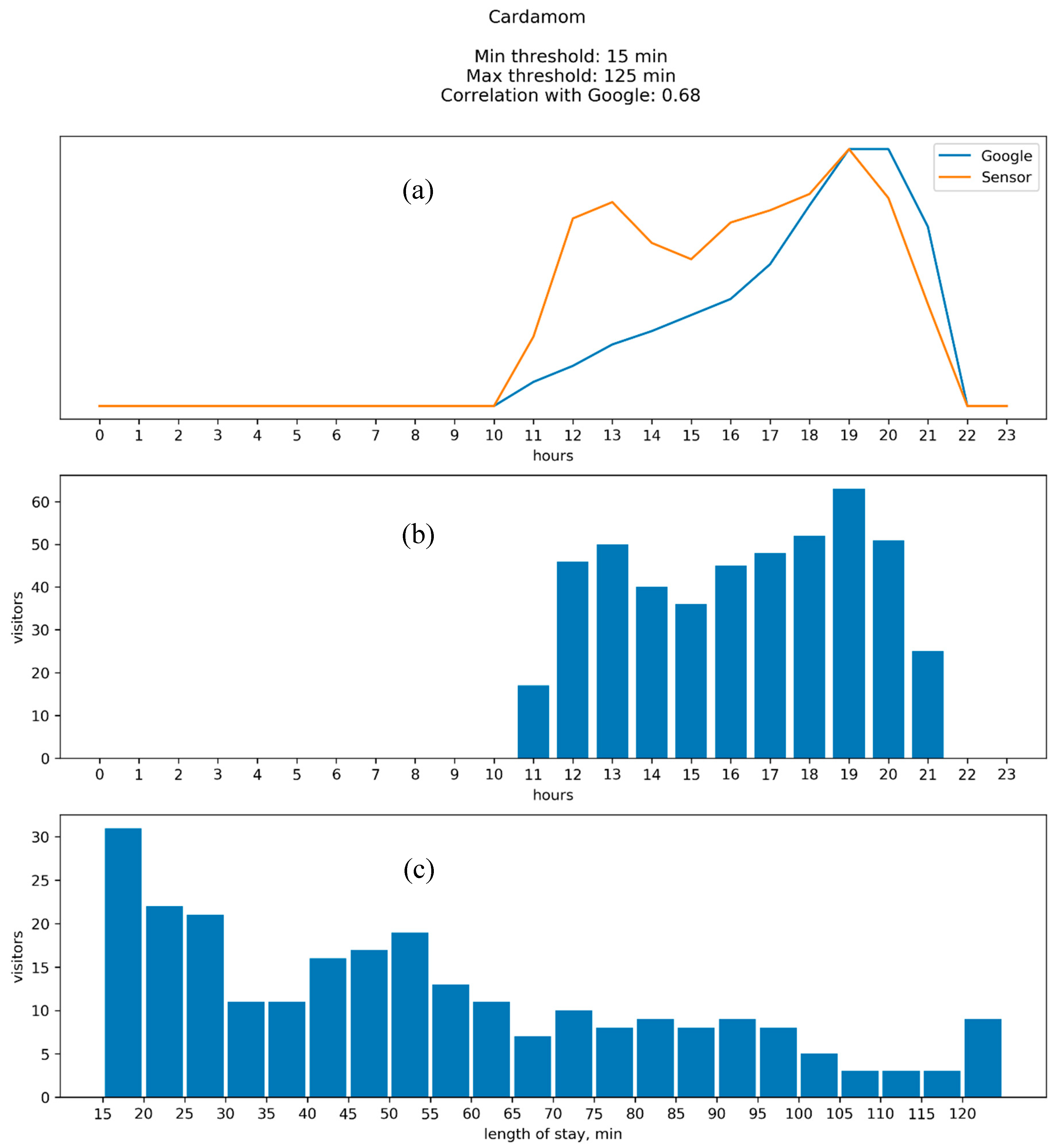
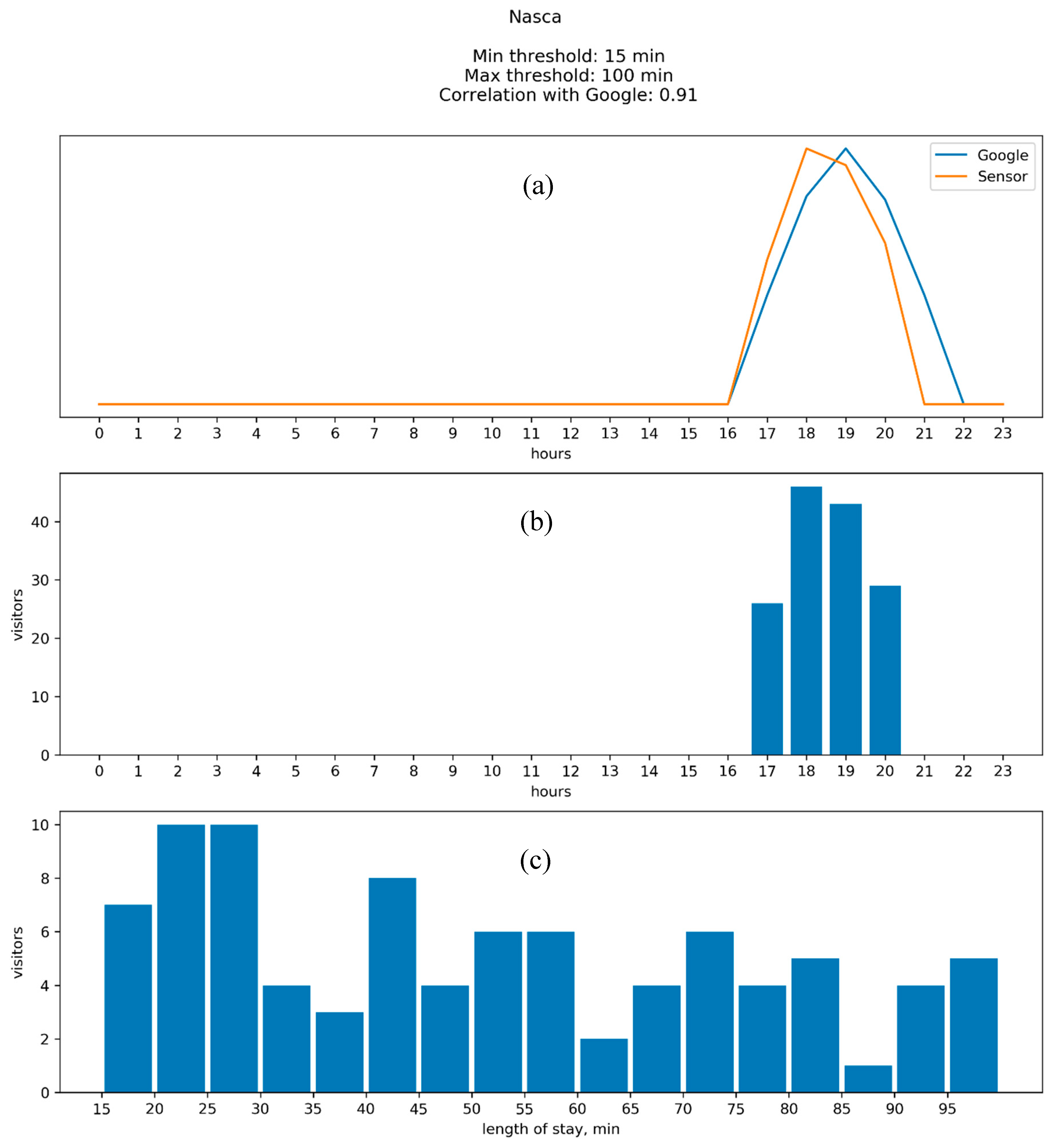
4.2. Results: Google vs. WiFi

In this section, the results of WiFi data collection and Google “Popular Times” are compared to each other. A Japanese restaurant, “Takumi”, is considered as the first case study (see Figure 13). We see that the result of WiFi data collection is broadly similar to Google “Popular Times”; nevertheless, a slight decline in the beginning of the operation is visible. This decline can be attributed to fluctuations in schedules of nearby organizations; for example, as this restaurant is close to the Technical University of Munich (TUM), changes in student activities can affect attendance. Furthermore, it is also possible to see that the number of visitors in this restaurant is quite high for this venue type. This might be a result of the impacts of other facilities located nearby. Nonetheless, the use of additional WiFi monitoring devices in the area can help to clear up this question.
Another venue, “Lo Studente”, shows an ideal correlation with Google (see Figure 14), which could be due to various factors. First of all, open architecture with several tables outside the main building can lead to appropriate signal reception by the WiFi monitor. Secondly, no big overlapping facilities exist in its vicinity.
The results of the remaining experiments are presented in Appendix B. Overall, the evaluation results have a wide range of outcomes. The majority of the venues considered have a correlation (between WiFi and Google “Popular Times”) at or higher than 0.9. However, a couple have much lower (0.68 and 0.41) correlations. The higher end of this range provides a very good proxy for the attendance of the venues. The lower end of this spectrum could still be valuable for a number of applications. The presented approach provides a cheap and scalable way to monitor venue attendance, with considerable prospects for valuable applications.

5. Concluding Remarks

With the rapid development of information and communication technologies (ICT), a large amount of spatiotemporal data is emerging, which can be used in transportation planning. For instance, the penetration of social media due to recent progress in broadband networks and mobile device technology has brought about an enhanced interest in location-based services for travel demand modeling applications and transport planning.
As a novel data source, Google “Popular Times” can give information on when a venue is mostly visited and live waiting time, as well as average visit duration, based on aggregated and undisclosed data from users who have opted to share their geotrace using their mobile devices. Such information can potentially improve real-time demand estimation for transportation planning applications. Nevertheless, up until now, “Popular Times” have not yet been widely used for this purpose. This research sets out to assess the possibility of using several services, including Google “Popular Times” and venue catalogues such as Yelp, as well as OpenStreetMap (OSM) data, for estimating venue popularity. Initially, data from the above-mentioned information sources were used to model venue popularity. We estimate venue occupancy at an hourly resolution level using two different classes of models, including linear regression with lasso regularization and gradient boosted regression (GBR). The predictions were made based on venue-related parameters (e.g., rating, comments) and locational properties (e.g., stores, hotels, attractions), showing an acceptable level of accuracy for the busiest hours of the day. We saw that the power of prediction for both classes of model increased with the transformation of the dependent variable. Since Google “Popular Times” data can merely represent relative venue attendance, a cost-effective WiFi microcontroller setup was developed and tested to measure the actual number of people attending a particular venue using WiFi device presence detection. The capability of Google “Popular Times” data in modeling venue popularity is quantified by comparing them with WiFi device presence detection. Our real-world tests in Munich, Germany, corroborated that the similarity between the results of WiFi data collection and Google “Popular Times” is relatively promising.
Following this finding, one question is which downstream analyses and inferences can be made based on this. In particular, can an estimate/prediction of attendance of people at a venue be used to infer their spending? Can it be used to assess public transport level of service or as a proxy for parking availability? Can it be used for developing anti-crowding monitoring strategies for use, among others, or mitigation of Covid-19 impacts? Could such real-time information be useful to guide consumers’ decisions about which venues to visit?
Future studies can take other factors and data sources into account which have not been involved in the present research, e.g., Twitter, Foursquare and Facebook data, along with detailed analysis of the contents of venue reviews. Moreover, a large scale WiFi data collection using a network of devices will need to be undertaken to increase the level of accuracy by diminishing the overlap of signals received from several venues located quite close to each other. Future research testing further regression and clustering techniques on data collected from different cities across the globe during long-term periods would be also interesting. In future investigations, it might be possible to use Bluetooth instead of WiFi as a sensor in the RPI zero and test several different matching algorithms to detect and track a device when it is connected to a sensor.

Author Contributions

Conceptualization, S.T., M.S. and C.A.; methodology, S.T. and C.A.; software, S.T.; writing—review and editing, S.T., M.S. and C.A.; supervision, C.A. All authors have read and agreed to the published version of the manuscript.

Funding

This research has been supported through the TUM International Graduate School of Science and Engineering-IGSSE (MO3 project).

Conflicts of Interest

The authors declare no conflict of interest.

Appendix A. Cross-Validation Method

Figure A1. Predicted vs. true values GBR example (outliers highlighted with yellow color). Horizontal axis—predicted y; vertical—true y.
Smartcities 03 00042 g0a1
Figure A2. GBR residuals example (outliers highlighted with yellow color). Horizontal axis—predicted y; vertical—normalized residuals.
Smartcities 03 00042 g0a2

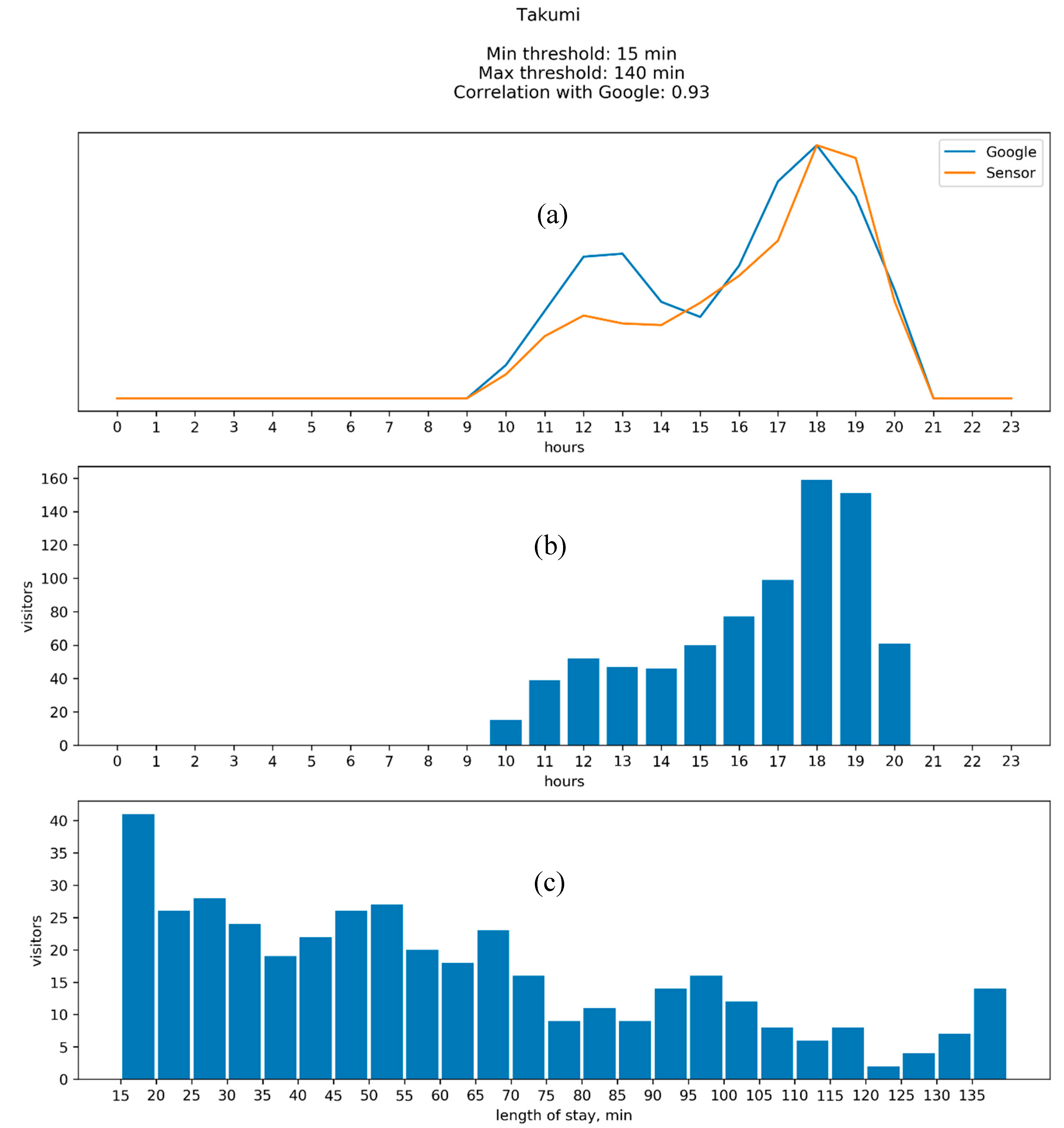
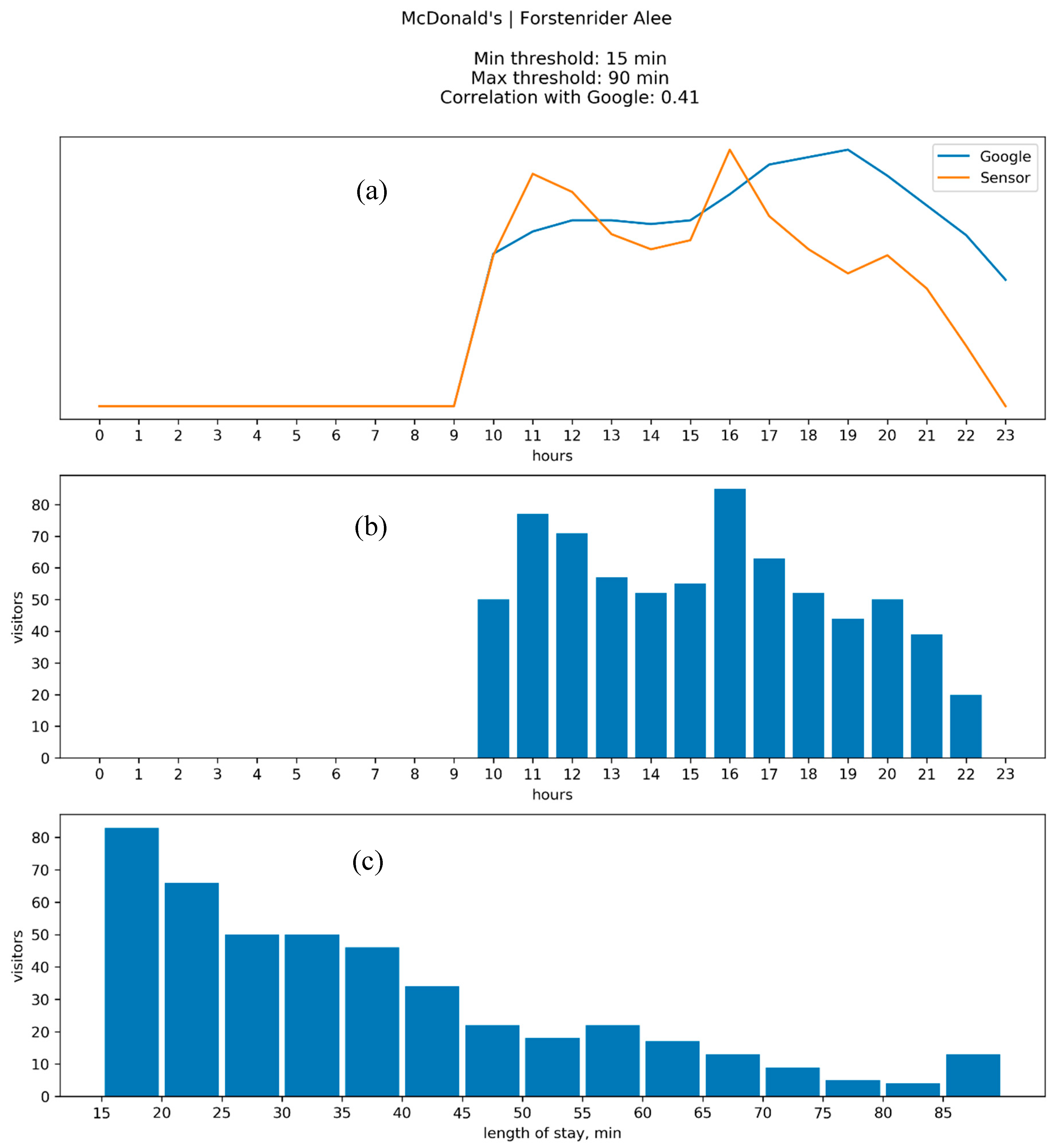
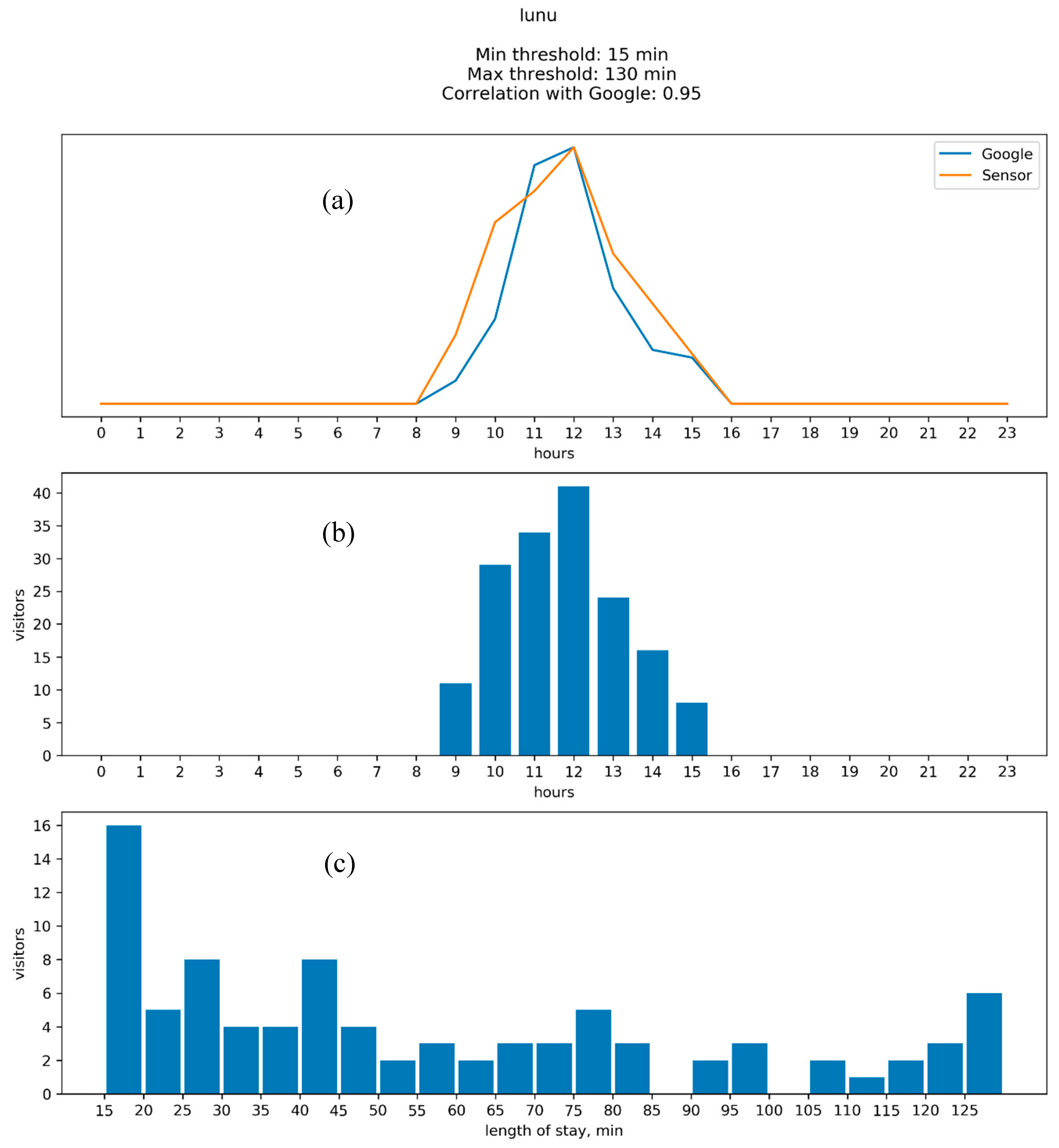
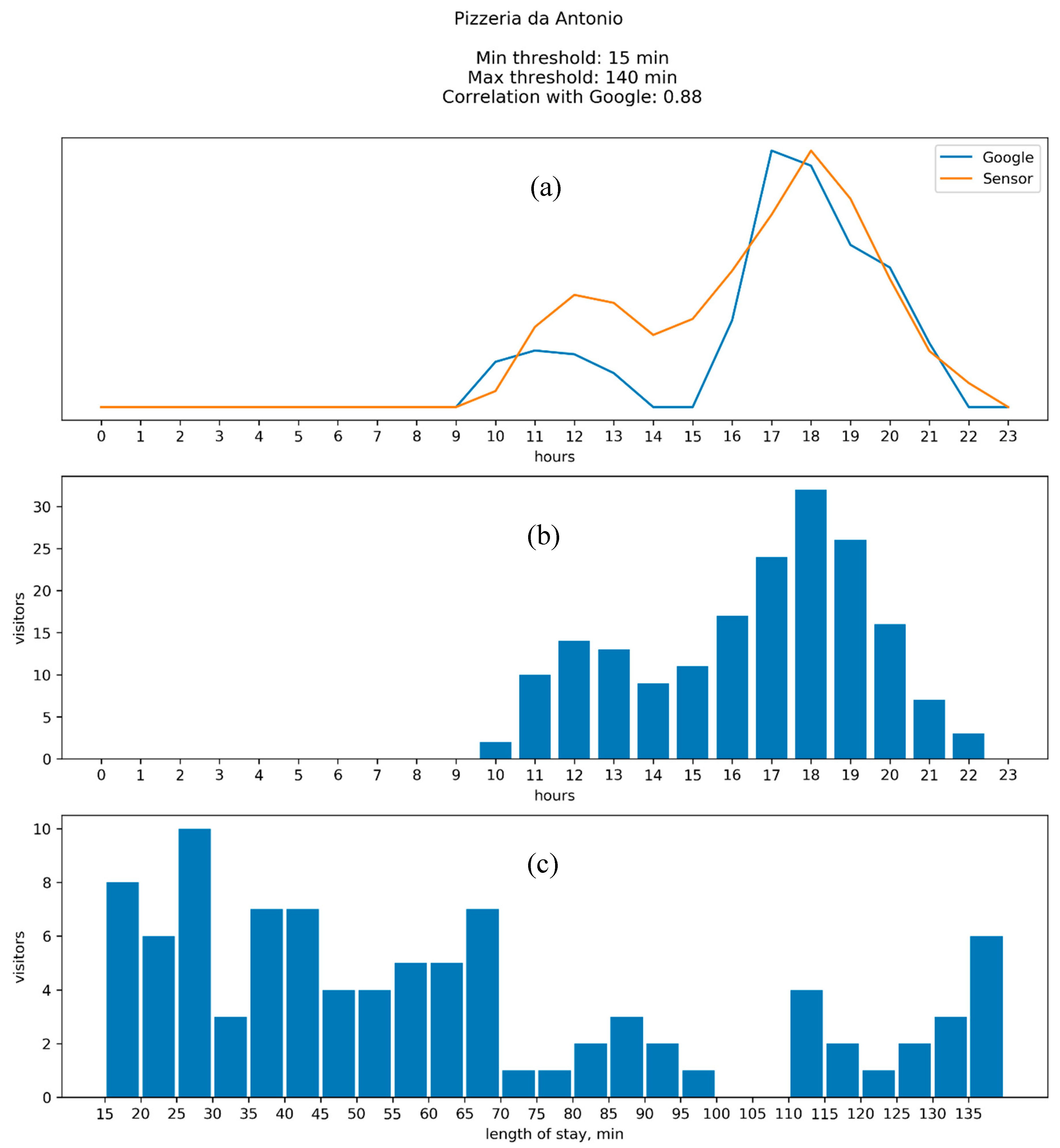
Appendix B. Comparison between the Results of WiFi Data Collection and Google “Popular Times”

Next, the experiments were performed on McDonald’s restaurant near Forstenrieder Alee. Spikes and drops were not visible on Google’s data on this venue. There was also a considerable decline in the sensor data compared to Google from 17 to 19 o’clock, which can be explained by the influence of surrounding organizations, detection problems due to building configuration and the fact that this venue has also a drive-through option, i.e., certain visitors may be filtered as passersby.
Figure A3. Venue attendance (“McDonald’s”, Forstenrieder Alee): (a) Google vs. WiFi; (b) visitors by time of day; (c) visitors’ length of stay distributions.
Smartcities 03 00042 g0a3
The “Iunu” cafeteria experienced roughly a similar pattern to Google. Regarding differences in the beginning and end of working hours, since it is located near a small park with several benches, sensors may have captured some people resting on them.
Figure A4. Venue attendance (“Iunu”): (a) Google vs. WiFi; (b) visitors by time of day; (c) visitors’ length of stay distributions.
Smartcities 03 00042 g0a4
Our experiments on “Pizzeria da Antonio” also indicate that the results of WiFi data collection and Google are acceptably much alike. A small drop in the beginning was because of the late start of data capture. A peak in the middle of the day may be a result of some overlapping venues. Nonetheless, this explanation is not robust enough with the existing data. That is, the number of visitors is relatively low; hence, even small groups of people may have affected the results.
Figure A5. Venue attendance (“Pizzeria da Antonio”): (a) Google vs. WiFi; (b) visitors by time of day; (c) visitors’ length of stay distributions.
Smartcities 03 00042 g0a5
The pattern of the cafeteria “Cardamom” was also interesting. The peak in the middle of the day in sensor data in comparison with Google “Popular Times” could be a result of an overlap of signals from several venues which are located quite close to each other. To mitigate this problem, it would be useful to install sensors near each venue and to define visitors of each exact one by analyzing signal strength as well.
Figure A6. Venue attendance (“Cardamom”): (a) Google vs. WiFi; (b) visitors by time of day; (c) visitors’ length of stay distributions.
Smartcities 03 00042 g0a6
Another example that shows a good correlation is the “Nasca” restaurant. This venue is located on a busy street between TUM and the Theresienstrasse subway station. Hence, several passersby may have been detected by the sensor at this place, especially in the beginning of the period.
Figure A7. Venue attendance (“Nasca”): (a) Google vs. WiFi; (b) visitors by time of day; (c) visitors’ length of stay distributions.
Smartcities 03 00042 g0a7

References

  1. Hu, W.; Jin, P.J. An adaptive hawkes process formulation for estimating time-of-day zonal trip arrivals with location-based social networking check-in data. Transp. Res. Part C Emerg. Technol. 2017, 79, 136–155. [Google Scholar] [CrossRef]
  2. Chaniotakis, E.; Antoniou, C.; Grau, J.M.S.; Dimitriou, L. Can Social Media data augment travel demand survey data? In Proceedings of the 2016 IEEE 19th International Conference on Intelligent Transportation Systems (ITSC), Rio de Janeiro, Brazil, 1–4 November 2016; pp. 1642–1647. [Google Scholar]
  3. Chaniotakis, E.; Antoniou, C.; Aifadopoulou, G.; Dimitriou, L. Inferring activities from social media data. Transp. Res. Rec. J. Transp. Res. Board 2017, 2666, 29–37. [Google Scholar] [CrossRef]
  4. Li, Y.; Steiner, M.; Wang, L.; Zhang, Z.-L.; Bao, J.; Steiner, M. Exploring venue popularity in foursquare. In Proceedings of the 2013 Proceedings IEEE INFOCOM, Turin, Italy, 14–19 April 2013; pp. 3357–3362. [Google Scholar]
  5. Yang, F.; Jin, P.J.; Cheng, Y.; Zhang, J.; Ran, B. Origin-destination estimation for non-commuting trips using location-based social networking data. Int. J. Sustain. Transp. 2014, 9, 551–564. [Google Scholar] [CrossRef]
  6. Scellato, S.; Noulas, A.; Lambiotte, R.; Mascolo, C. Socio-spatial properties of online location-based social networks. In Proceedings of the Fifth International AAAI Conference on Weblogs and Social Media, Barcelona, Spain, 17–21 July 2011. [Google Scholar]
  7. Muhammad, R.; Zhao, Y.; Liu, F. Spatiotemporal analysis to observe gender based check-in behavior by using social media big data: A case study of Guangzhou, China. Sustainability 2019, 11, 2822. [Google Scholar] [CrossRef] [Green Version]
  8. Popular Times and Visit Duration-Google My Business Help Google. Available online: https://www.google.com/maps (accessed on 1 January 2018).
  9. Tafidis, P.; Teixeira, J.; Bahmankhah, B.; Macedo, E.; Guarnaccia, C.; Coelho, M.C.; Bandeira, J.M. Can Google maps popular times be an alternative source of information to estimate traffic-related impacts? Transp. Res. Board 2018, 97, 1–8. [Google Scholar]
  10. Meeks, W.; Dasgupta, S. Geospatial information utility: An estimation of the relevance of geospatial information to users. Decis. Support Syst. 2004, 38, 47–63. [Google Scholar] [CrossRef]
  11. Kisilevich, S.; Keim, D.; Rokach, L. A GIS-based decision support system for hotel room rate estimation and temporal price prediction: The hotel brokers’ context. Decis. Support Syst. 2013, 54, 1119–1133. [Google Scholar] [CrossRef] [Green Version]
  12. Wang, L.; Gopal, R.; Shankar, R.; Pancras, J. On the brink: Predicting business failure with mobile location-based checkins. Decis. Support Syst. 2015, 76, 3–13. [Google Scholar] [CrossRef]
  13. Rodas, D.D. Identification of Spatio-Temporal Factors Affecting Arrivals and Departures of Shared Vehicles. Master’s Thesis, Technical University of Munich, Munich, Germany, 2017. [Google Scholar]
  14. Willing, C.; Klemmer, K.; Brandt, T.; Neumann, D. Moving in time and space–location intelligence for carsharing decision support. Decis. Support Syst. 2017, 99, 75–85. [Google Scholar] [CrossRef]
  15. Chen, Y.; Mahmassani, H.S.; Frei, A. Incorporating social media in travel and activity choice models: Conceptual framework and exploratory analysis. Int. J. Urban Sci. 2017, 22, 180–200. [Google Scholar] [CrossRef]
  16. Hasan, S.; Ukkusuri, S.V. Urban activity pattern classification using topic models from online geo-location data. Transp. Res. Part C Emerg. Technol. 2014, 44, 363–381. [Google Scholar] [CrossRef]
  17. Hasnat, M.; Hasan, S. Identifying tourists and analyzing spatial patterns of their destinations from location-based social media data. Transp. Res. Part C Emerg. Technol. 2018, 96, 38–54. [Google Scholar] [CrossRef]
  18. Llorca, C.; Ji, J.; Molloy, J.; Moeckel, R. The usage of location based big data and trip planning services for the estimation of a long-distance travel demand model. Predicting the impacts of a new high speed rail corridor. Res. Transp. Econ. 2018, 72, 27–36. [Google Scholar] [CrossRef]
  19. Yang, F.; Ding, F.; Qu, X.; Ran, B. Estimating Urban Shared-Bike Trips with Location-Based Social Networking Data. Sustainability 2019, 11, 3220. [Google Scholar] [CrossRef] [Green Version]
  20. Yang, L.; Durarte, C.M. Identifying tourist-functional relations of urban places through foursquare from Barcelona. GeoJournal 2019. [Google Scholar] [CrossRef]
  21. Liu, X.; Andris, C.; Rahimi, S. Place niche and its regional variability: Measuring spatial context patterns for points of interest with representation learning. Comput. Environ. Urban Syst. 2019, 75, 146–160. [Google Scholar] [CrossRef]
  22. Weerdenburg, D.V.; Scheider, S.; Adams, B.; Spierings, B.; Zee, E.V.D. Where to go and what to do: Extracting leisure activity potentials from Web data on urban space. Comput. Environ. Urban Syst. 2019, 73, 143–156. [Google Scholar] [CrossRef]
  23. Deveaud, R.; Albakour, M.-D.; Macdonald, C.; Ounis, I. Experiments with a venue-centric model for personalisedand time-aware venue suggestion. In Proceedings of the 24th ACM International on Conference on Information and Knowledge Management-CIKM’15, Melbourne, Australia, 19–23 October 2015; pp. 53–62. [Google Scholar]
  24. Manotumruksa, J.; MacDonald, C.; Ounis, I. Predicting contextually appropriate venues in location-based social networks. In Proceedings of the International Conference of the Cross-Language Evaluation Forum for European Languages, Évora, Portugal, 5–8 September 2016; pp. 96–109. [Google Scholar]
  25. Noulas, A.; Scellato, S.; Lathia, N.; Mascolo, C. Mining user mobility features for next place prediction in location-based services. In Proceedings of the 2012 IEEE 12th International Conference on Data Mining, Brussels, Belgium, 10 December 2012; pp. 1038–1043. [Google Scholar]
  26. Perner, P. Advances in data mining. applications and theoretical aspects. Comput. Vis. 2013, 7987, 107–121. [Google Scholar] [CrossRef]
  27. Yoshimura, Y.; Krebs, A.; Ratti, C. Noninvasive bluetooth monitoring of visitors’ length of stay at the louvre. IEEE Pervasive Comput. 2017, 16, 26–34. [Google Scholar] [CrossRef]
  28. Nunes, N.; Ribeiro, M.; Prandi, C.; Nisi, V. Beanstalk: A community based passive wi-fi tracking system for analysing tourism dynamics. In Proceedings of the ACM SIGCHI Symposium on Engineering Interactive Computing Systems, Lisbon, Portugal, 26–29 June 2017; pp. 93–98. [Google Scholar]
  29. Pang, Y.; Kashiyama, T.; Yabe, T.; Tsubouchi, K.; Sekimoto, Y. Development of people mass movement simulation framework based on reinforcement learning. Transp. Res. Part C Emerg. Technol. 2020, 117, 102706. [Google Scholar] [CrossRef]
  30. Schulz, M.; Wegemer, D.; Hollick, M. Nexmon: The c-based firmware patching framework. Res. Gate 2017. [Google Scholar] [CrossRef]
  31. IEEE Standards Association. IEEE Standard for Information Technology–Telecommunications and Information Exchange Between Systems–Local and Metropolitan Area Networks–Specific Requirements; IEEE: New York, NY, USA, 2010; IEEE Std 802 (Part 11: Wireless LAN Medium Access Control (MAC) and Physical Layer (PHY) specifications Amendment 6: Wireless. Access in Vehicular Environments). [Google Scholar]
  32. Ji, Y.; Zhao, J.; Zhang, Z.; Du, Y. Estimating bus loads and OD flows using location-stamped farebox and Wi-Fi signal data. J. Adv. Transp. 2017, 2017, 1–10. [Google Scholar] [CrossRef] [Green Version]
Figure 1. The general framework of the venue popularity modeling and measuring in the present work (authors’ elaboration).
Smartcities 03 00042 g001
Figure 2. Screenshot of Yelp (yelp.com).
Smartcities 03 00042 g002
Figure 3. Screenshot of Google Maps (google.com/maps).
Smartcities 03 00042 g003
Figure 4. Screenshot of Google “Popular Times” section (google.com/maps).
Smartcities 03 00042 g004
Figure 5. Box–Cox parameter selection (GBR, 400 m dependent zone).
Smartcities 03 00042 g005
Figure 6. Box–Cox parameter selection (multiple linear regression, 400 m dependent zone).
Smartcities 03 00042 g006
Figure 7. Most important variables within all GBR models (without transformation).
Smartcities 03 00042 g007
Figure 8. Most important variables within all GBR models (log transformation).
Smartcities 03 00042 g008
Figure 9. Most important variables within all GBR models (Box–Cox transformation).
Smartcities 03 00042 g009
Figure 10. Difference between transformed models and models without transformation (GBR).
Smartcities 03 00042 g010
Figure 11. Difference between GBR and linear models with Box–Cox transformation.
Smartcities 03 00042 g011
Figure 12. Photo of the microcontroller setup.
Smartcities 03 00042 g012
Figure 13. Venue attendance (“Takumi”): (a) Google vs. WiFi; (b) visitors by time of day; (c) visitors’ length of stay distributions.
Smartcities 03 00042 g013
Figure 14. Venue attendance (“Lo Studente”): (a) Google vs. WiFi; (b) visitors by time of day; (c) visitors’ length of stay distributions.
Smartcities 03 00042 g014
Table 1. List of primary data sources.
Yelphttps://www.yelp.com
Google Mapshttps://www.google.com/maps
Google Location APIhttps://developers.google.com/maps/documentation/geolocation/intro
Overpass APIhttps://wiki.openstreetmap.org/wiki/Overpass_API
OSM Dumphttps://www.geofabrik.de (pbf file)
Populationhttps://www.zensus2011.de (German nationwide census, 2011)
Workplaceshttps://www.muenchen.de (Munich, 2016)
Table 2. Variable descriptions.
Variable NameDescription
-Index
NameName of venue
lat_convLatitude
lon_convLongitude
Price_indexPrice level from Yelp
compound_ratingWeighted sum of ratings obtained from Yelp and Google Maps
total_reviewsSum of reviews at Yelp and Google Maps
*Type of amenity (e.g., cafe_fastfood)
*Tags attached (e.g., Caribbean)
roads_*
nodes_*
ways_*
OSM data on length of different classes of roads and number of venues within prespecified area
workplacesWorkplaces data within prespecified area
populationPopulation data within prespecified area
*Working hours
(−2 h, −1 h, current hour, +1 h, +2 h)
*Venue popularity data 24 h/7 days (e.g., (‘sun’, 1))
Table 3. List of Python libraries.
SeleniumEmulation of user activity in browser
Beautiful SoupParsing of HTML and XML documents
PandasHigh performance and easy to use data structures and data analysis tools
GeopandasExtension of pandas library for work with spatial data
OsmreadReading of OpenStreetMap XML and PBF data files
OsmnxRetrieving, constructing, analyzing and visualizing street networks
Scikit-learnTools for data mining and data analysis
TslearnTools for data mining and data analysis of time series
MatplotlibData visualization
StatsModelsEstimation and evaluation of statistical models
Table 4. Gradient boosted regression results (400 m dependent zone; median values).
No TransformationBox–Cox ( λ = 0)Box–Cox ( λ = −1.4)
Mean Squared Error (MSE)119.290.590.02
R 2 0.500.590.61
MSE (Coefficient of Variation [CV])154.160.760.03
R 2 (CV)0.340.450.47
MSE (test set)162.340.700.02
R 2 (test set)0.330.470.49
Table 5. Multiple linear regression with lasso results (400 m dependent zone; median values).
No TransformationBox–Cox ( λ = 0)Box–Cox ( λ = −0.2)
MSE141.800.720.34
R 2 0.420.460.46
MSE (CV)153.890.780.39
R 2 (CV)0.340.430.43
MSE (test set)161.830.750.38
R 2 (test set)0.320.450.45
Table 6. The price of each item used in the microcontroller setup (2018, amazon.de).
ItemCost, EUR
Raspberry Pi Zero W10
Micro SD card (16 GB)6.49
Power Bank (5000 mAh)8.99

