Model Predictive Control of a Road Junction

Abstract

This paper presents a model predictive control (MPC) approach for optimally managing the traffic light (TL) signals at a road junction. The objective is to improve queue balancing compared to traditional control strategies where TL signals are periodic. The resulting MPC optimization problem is of quadratic mixed-integer nature. The proposed approach is validated via simulations based on a real scenario.

1. Introduction

Improving traffic light (TL) control can bring significant impacts in terms of reducing traffic congestion in cities, reducing emissions, improving travel experience, etc. Intelligent TL control is an intensively studied area of research. The classic control approach, still widely used today, is to have fixed TL timings, optimized based on the statistical properties of the traffic flows to be controlled. This strategy has the merit of being extremely simple to implement, requiring also no particular sensing and computing equipment to be installed. Several improved TL control strategies have been proposed in the literature. A review of them can be found, e.g., in [1,2,3]. Advanced techniques used recently include deep reinforcement learning [4], game theory [5], evolutionary algorithm [6], fuzzy control [7], model predictive control (MPC) [8] and others. This work proposes an MPC control strategy based on quadratic mixed-integer optimization. Relevant related works in literature include [9,10], in which the authors propose an MPC framework for intelligent traffic signal control in a road network. The objective is to reduce the total number of vehicles in the network (i.e., the total traffic). The MPC algorithm in [10] is based on mixed-integer linear programming, which results in feasible solving times. Linear programming is applied in [10] since in that study the objective is to minimize the sum of the queues in the network. The aim of the present work instead is to minimize and as well to balance the queues, which is achieved with a quadratic objective function. Furthermore, compared to [10], the present paper proposes a more accurate, nonlinear queue equation, in which the outflow from a queue is a function of the outflow rate (which in turn depends on the traffic light signal and the queue length), rather than simply a fraction of the queue (compare (10) with (3) in [10]). In more recent work [11], the authors propose a model-free adaptive predictive control for phase splits of urban traffic networks. The goal is to minimize the number of vehicles in the network. The authors derive the nonlinear traffic network dynamical model and then linearize it to derive a simple MPC based signal split strategy. In [11], dynamic linearization is achieved by computing at each control step the Jacobian of the traffic network nonlinear model. In the present work instead, an effort is done to derive accurate, nonlinear queue equations which can be exactly linearized through the inclusion of additional auxiliary Boolean and continuous variables (e.g., see (10) to (15)). Reference [12] proposes a similar control strategy, also incorporating relevant rules from the US National Electrical Manufacturing Association (NEMA) standards for the sector. Reference [13] extends the above works by proposing a distributed MPC framework (based on the dual decomposition method) for urban traffic network control. The authors show that the approach significantly reduces computation times and queue lengths. A similar approach will be pursued in future works to derive a decentralized version of the present work, for application to traffic network control scenarios. Furthermore, compared to [13], the present work provides a more accurate modelling of the queue balance equation, for the same reasons discussed above. In addition, in [13] the change of the queue length depends on the cycle time (i.e., the sum of the traffic light phases duration), while in the present work the cycle time is variable and adjusted by the controller in order to best match the traffic conditions. Reference [14] proposes a multi-objective optimal MPC of signals in urban traffic networks. The optimization goals considered are: maximizing system throughput, minimizing traveling delays, maximizing intersection crossing volume, avoiding spillbacks, enhancing traffic safety. The optimal solutions are found by resorting to genetic algorithms and Pareto multi-objective optimization theory. Reference [15] proposes a distributed event-triggered MPC strategy for traffic signals control in urban traffic networks. The main goal is to minimize the total time spent by the cars in the network. Contrary to traditional MPC, in which re-optimization is periodic and time-driven, the controller proposed in [15] performs re-optimization (i.e., it computes a new control solution) only when specific conditions are met, which avoids redundant computation and communication efforts. A similar approach could be embedded in the algorithm presented here in future works.

The main goal of the present paper is to show how the usage of the proposed control algorithm can improve the performance of the road junction, as captured by a set of key performance indicators (KPIs), such as: queue balancing (the focus of the present work), minimization of the total vehicles’ waiting time, throughput of vehicles (i.e., vehicles processed over time), etc. Compared to the above-mentioned works and the general existing literature, the present work is more focused on the control of the single road junction, for which a more fine-grained mathematical modelling is introduced, which enables more accurate control and optimization of different KPIs, both driver-related (e.g., time spent at the road junction) and network related (e.g., throughput, balancing of the queues, etc.). In particular, as discussed above, this study introduces a different and more accurate nonlinear model of the queue length (which is the most important equation in this application area). The proposed queue model is nonlinear, however, it is also shown how it can be exactly linearized by introducing additional auxiliary variables. This allows keeping a linear formulation of the problem constraints, which reduces the computational complexity of the MPC problem. In addition, other detailed equations needed to realistically model the traffic light functioning logic are presented as well, such as the dynamics of the duration of the traffic light signs (8), the phases transition constraints (2)–(4) and the conflict avoiding constraints (17).

The rest of the paper is organized as follows. Section 2 presents the MPC control approach adopted in the paper. Section 3 presents the optimization problem at the basis of the proposed MPC approach: the optimization problem includes constraints to model the road junction, and a target function to capture the optimization goals. Section 4 presents simulation results based on a real scenario. Finally, in Section 5 conclusions and future works are presented.

2. MPC Control Logic

The problem is set up in discrete time, with T denoting the sampling time in seconds. L denotes the number of traffic lights and $j\in [1,2,\dots ,L]$ the generic traffic light. According to the MPC control method, at the generic current time $k=1,2,\dots$, the TLs control signals $g_{k,j}$, $y_{k,j}$, $r_{k,j}$ (respectively, green, yellow and red) to be actuated are found by solving a constrained optimization problem defined over a time window of N time steps into the future, i.e., from time k to time $k+N-1$ (the time interval $[k,k+N-1]$ is the so called prediction horizon). The optimal control problem to be solved at the generic time k is built based on the boundary conditions of the road junction, as acquired from the feedback from sensors deployed on the field or from the vehicle (considering cooperative scenarios). In particular, the main information that the MPC controller needs to measure or estimate at every k is the length of the queues. The MPC control loop is summarised in the follow.

In the next section, the mathematical formulation of the optimal control problem that is built and solved in Step 2 of Algorithm 1 is presented. The goal of the control problem is to derive the optimal TL timing, based on specific optimization criteria, and subject to a number of constraints that model the TL junction and that enforce a correct timing of the TLs.

Algorithm 1: MPC control of a road junction.

3. MPC Road Junction Optimization Problem

We derive in the following a linear mathematical model for the road junction. The model captures all the constraints that need to be respected to enforce a correct functioning of the road junction and the TLs. The model is defined over the prediction horizon $[k,k+N-1]$.

In the following, the index $j\in [1,2,\dots ,L]$ denotes a generic TL of the road junction, while the index i is used to denote a generic time step in the prediction horizon (i.e., $i\in [k,k+N-1]$).

3.1. Model of a TL

The state of a TL j at time i is given by the triple of Boolean variables $\{g_{i,j},y_{i,j},r_{i,j}\}$, green, yellow and red status, respectively. It must be:

$$g_{i,j}+y_{i,j}+r_{i,j}=1,\forall i,j.$$

(1)

The right order of the transition of the lights from green to yellow to red is enforced by the following three constraints, which avoid, respectively, the transition from green to red, from red to yellow, and from yellow to green:

$$r_{i+1,j}\le 1-g_{i,j},\forall i,j,$$

(2)

$$y_{i+1,j}\le 1-r_{i,j},\forall i,j,$$

(3)

$$g_{i+1,j}\le 1-y_{i,j},\forall i,j.$$

(4)

For example, it is seen from (2) that if it is $g_{i,j}=1$, then it must be $r_{i+1,j}=0$.

Next, for safety reasons, a minimum duration time for the yellow is set. To this end, an auxiliary variable $t_i^y$ is introduced, to indicate the duration (in number of time steps) of the current yellow cycle up to time i (the duration is zero if the sign is not yellow, greater than zero otherwise).

$$t_{i+1,j}^y=t_{i,j}^y+y_{i,j}-t_{i,j}^y{y}_{i,j}^{\uparrow },\forall i\in [k,k+N-2],j,$$

(5)

where $y_{i,j}^{\uparrow }$ is a Boolean variable equal to one when and only when the state transits from green to yellow. This behaviour for $y_{i,j}^{\uparrow }$ is achieved via the inclusion of the following constraints:

$$y_{i+1,j}-y_{i,j}\le (1+ϵ)y_{i+1,j}^{\uparrow }\le y_{i+1,j}-y_{i,j}+1,\forall i\in [k,k+N-2],j,$$

(6)

with $ϵ$ an arbitrary small positive constant. In fact, when there is a transition from green to yellow, i.e., when $y_{i+1,j}-y_{i,j}=1$, (6) forces $y_{i+1,j}^{\uparrow }$ to one. On the other hand, when $y_{i+1,j}-y_{i,j}=0$ (i.e., when the yellow sign does not vary) or when $y_{i+1,j}-y_{i,j}=-1$ (i.e., the sign goes from yellow to red), then (6) forces $y_{i+1,j}^{\uparrow }$ to zero, which is exactly the behaviour sought for $y_{i+1,j}^{\uparrow }$.

As explained, e.g., in [16], the nonlinear term $t_{i,j}^y{y}_{i,j}^{\uparrow }$ in (5), which is the product of a continuous variable and a Boolean variable, can be equivalently written in linear form by including an auxiliary variable ${\widehat{t}}_{i,j}^y$ and the following auxiliary constraints:

$$\left\{\begin{array}{c}0\le {\widehat{t}}_{i,j}^y\le t_{i,j}^{y,max}{y}_{i,j}^{\uparrow }\hfill \\ t_{i,j}^y-(1-y_{i,j}^{\uparrow })t_{i,j}^{y,max}\le {\widehat{t}}_{i,j}^y\le t_{i,j}^y,\forall i,j.\hfill \end{array}\right.$$

(7)

It can be verified indeed that, with the above constraints it is ${\widehat{t}}_{i,j}^y=t_{i,j}^y$ when $y_{i,j}^{\uparrow }=1$, and ${\widehat{t}}_{i,j}^y=0$ when $y_{i,j}^{\uparrow }=0$ (i.e., ${\widehat{t}}_{i,j}^y=t_{i,j}^y{y}_{i,j}^{\uparrow }$, as sought). Hence (5) is rewritten simply as:

$$t_{i+1,j}^y=t_{i,j}^y+y_{i,j}-{\widehat{t}}_{i,j}^y,\forall i\in [k,k+N-2],j,$$

(8)

from which it is seen that, when $y_{i,j}=1$, the duration of the current yellow cycle is increased by one, and when $y_{i,j}^{\uparrow }=1$, (i.e., the sign switches from green to yellow) $t_{i,j}^y$ is reset to zero.

Finally, the following constraints ensure that a minimum duration of the yellow sign is respected:

$$1-\frac{t_{i,j}^y}{t_{i,j}^{y,min}}\le y_{i,j},\forall i,j,$$

(9)

where $t_{i,j}^{y,min}$ denotes the minimum duration of the yellow sign. In fact, as long as $t_{i,j}^y\le t_{i,j}^{y,min}$, variable $y_{i,j}$ is forced by (9) to one (notice also from (5) that, since $y_{i+1,j}^{\uparrow }$ is reset when the sign switches from green to yellow, it is always $t_{i,j}^y\ge t_{i,j}^{y,min}$ when the sign is not yellow).

3.2. Model of the Queue at a TL

Number of Vehicles in Queue

Let $n_{i,j}\ge 0$ denote the number of vehicles in queue at time i at the TL j. Let $v_{i,j}^{in}$ and $v_{i,j}^{out}$ denote, respectively, the rate of vehicles (vehicles per seconds) entering the queue and exiting the queue at time i. The following approximated dynamics of the queue is derived:

$$n_{i+1,j}=n_{i,j}+T(v_{i,j}^{in}-v_{i,j}^{out}{g}_{i,j}),\forall i\in [k,k+N-2],j.$$

(10)

In practice, $v_{i,j}^{out}$ and $v_{i,j}^{in}$ are time varying (they depend on the traffic conditions) and need to be estimated based on measurements of the real time traffic flow (e.g., by using conventional vehicle detectors for signal operation, vehicle-to-infrastructure technology, etc. (see, e.g., [17,18]). Note that the two rates are equal when there is no queue and the TL is green:

$$v_{i,j}^{out}=v_{i,j}^{in}\mathrm{if}{n}_{i,j}=0\mathrm{and}{g}_{i,j}=1,\forall i,j.$$

(11)

On the other hand, when $n_{i,j}\ge 0$ and the TL is green, $v_{i,j}^{out}$ will be equal to an “escape rate” which will depend on the characteristics of the vehicles, the road (e.g., it will be higher for straight roads, compared to closed curves), etc. This rate as well can be estimated based on measurements.

To model the above behaviour related to $v_{i,j}^{out}$, a Boolean variable, ${\overline{n}}_{i,j}$, is introduced to indicate if $n_{i,j}$ is zero (in which case it is ${\overline{n}}_{i,j}=0$ as well) or greater than zero (in which case it is ${\overline{n}}_{i,j}=1$). This is easily achieved by introducing the following constraints:

$$n_{i,j}\le M{\overline{n}}_{i,j},{\overline{n}}_{i,j}\le M{n}_{i,j},\forall i,j,$$

(12)

where M is a large positive number (larger than the maximum value that $n_{i,j}$ can take).

Therefore, when ${\overline{n}}_{i,j}=0$ (i.e., there is no queue) and $g_{i,j}=1$ it is $v_{i,j}^{out}=v_{i,j}^{in}$, while when ${\overline{n}}_{i,j}=1$ and $g_{i,j}=1$ it is $v_{i,j}^{out}=v_{i,j}^{esc}$, where $v_{i,j}^{esc}$ is the above-introduced escape rate of vehicles at the TL.

Next, two auxiliary continuous variables are introduced to capture the two above “and” products: ${\widehat{g}}_{i,j}:={\overline{n}}_{i,j}{g}_{i,j}$ and ${\check{g}}_{i,j}:=(1-{\overline{n}}_{i,j})g_{i,j}$. It is easily verified that the desired behaviour for ${\check{g}}_{i,j}$ and ${\widehat{g}}_{i,j}$ is obtained with the following constraints (see, e.g., [19]):

$${\widehat{g}}_{i,j}:={\overline{n}}_{i,j}{g}_{i,j}\mathrm{is}\mathrm{equivalent}\mathrm{to}\left\{\begin{array}{c}{\widehat{g}}_{i,j}\le {\overline{n}}_{i,j},\hfill \\ {\widehat{g}}_{i,j}\le g_{i,j},\hfill \\ {\widehat{g}}_{i,j}\ge {\overline{n}}_{i,j}+g_{i,j}-1,\forall i,j,\hfill \end{array}\right.$$

(13)

$${\check{g}}_{i,j}:=(1-{\overline{n}}_{i,j})g_{i,j}\mathrm{is}\mathrm{equivalent}\mathrm{to}\left\{\begin{array}{c}{\check{g}}_{i,j}\le 1-{\overline{n}}_{i,j},\hfill \\ {\check{g}}_{i,j}\le g_{i,j},\hfill \\ {\check{g}}_{i,j}\ge -{\overline{n}}_{i,j}+g_{i,j},\forall i,j.\hfill \end{array}\right.$$

(14)

Hence (10) can be rewritten as:

$$n_{i+1,j}=n_{i,j}+T[v_{i,j}^{in}-v_{i,j}^{in}{\check{g}}_{i,j}-v_{i,j}^{esc}{\widehat{g}}_{i,j}],\forall i\in [k,k+N-2],j.$$

(15)

Finally, it is necessary to add a last continue and non-negative auxiliary variable to (15) in order to prevent that $n_{i,j}$ takes negative values:

$$n_{i+1,j}=n_{i,j}+T[v_{i,j}^{in}-v_{i,j}^{in}{\check{g}}_{i,j}-v_{i,j}^{esc}{\widehat{g}}_{i,j}]+s_{i,j},\forall i\in [k,k+N-2],j.$$

(16)

In other terms, $s_{i,j}$ acts as a feasibility slack variable that prevents that infeasibility arises due to $n_{i+1,j}$ becoming negative in specific conditions, e.g., when $n_{i,j}=1$, $v_{i,j}^{in}-v_{i,j}^{esc}\le -1$ vehicles/second and $T\ge 1$ second: this would result in infeasibility, because $n_{i+1,j}$ as computed by (15) would be negative. A dedicated term will be included in the objective function to ensure that $s_{i,j}$ is greater than zero only when needed (i.e., only to prevent infeasibility). More sophisticated modelling choices for $v_{i,j}^{out}$ are possible. For example, $v_{i,j}^{out}$ could be taken as an increasing function of the current duration of the green sign.

Starting from $n_{i,j}$, other interesting variables can be derived. For example, the approximate length of the queues (in meters), as $l_{i,j}=n_{i,j}l$, where l denotes the average space occupied in queue by a vehicle. Including this variable allows, e.g., including constraints on the maximum length admissible for a given queue, for example to minimize the possibility that a queue stretches to, and blocks, another traffic junction. Another quantity that can be derived from $n_{i,j}$ is an estimate of the waiting time $d_{i,j}$ for a vehicle entering queue j at time i, which can be approximated via the Little law [20] as $d_{i,j}=n_{i,j}/v_{i,j}^{out},\forall i,j$, where $v_{i,j}^{out}$ should be the average escape velocity. The Little law states that the waiting time in a queue is given by the number of items in the queue (vehicles) over the average exit rate (vehicles/seconds). The average vehicle exit rate can be a moving average of the observed exit rate. Future works will focus on a more accurate estimation of the waiting time for every vehicle in the queue. Finally, another interesting variable is the total amount of vehicles going through the TL at the generic time interval i, which can be computed as $p_{i,j}=T(v_{i,j}^{in}{\check{g}}_{i,j}+v_{i,j}^{esc}{\widehat{g}}_{i,j})$. This can be seen as the number of vehicles “processed” by the algorithm at lane j at time i.

3.3. Conflict Avoiding Constraints

A set of lanes ${\mathcal{C}}_i$ with $|{\mathcal{C}}_i|>1$ is called “conflicting” if any two lanes in the set intersect (i.e., vehicles flowing in any two lanes could potentially collide). For example, there are three conflicting sets in the junction in Figure 1: ${\mathcal{C}}_1=\{1,3\}$, ${\mathcal{C}}_2=\{1,2,4\}$ and ${\mathcal{C}}_3=\{2,5\}$. Denote with $\mathcal{C}$ the set of all conflicting sets. The following constraint states that at maximum one TL per conflicting set can be green or yellow at any time.

$$\sum _{j\in {\mathcal{C}}_i}(g_{i,j}+y_{i,j})\le 1\forall i\in [k,k+N-1],{\mathcal{C}}_i\in \mathcal{C}$$

(17)

3.4. Objective Function

Optimization is focuses at balancing the queues at the TLs. The objective function to be minimized is:

$$J_N=\sum _{i=0}^{N-1}\sum _{j=1}^L\left({\alpha }_j{n}_{i,j}^2+M{s}_{i,j}^2\right),$$

(18)

where ${\alpha }_j$ is a positive weight and M a large positive number.

The term ${\alpha }_j{n}_{i,j}^2$ is to minimize/balance the length of the queues at the road junction. The term $M{s}_{i,j}^2$ is to minimize the slack variable of constraint (16).

3.5. Overall MPC Optimization Problem

The overall optimization problem (i.e., the one build and solved at step 2 of Algorithm 1) is:

$$\mathrm{argmin}\left\{J_N=\sum _{i=0}^{N-1}\sum _{j=1}^L\left({\alpha }_j{n}_{i,j}^2+M{s}_{i,j}^2\right)\right\},$$

(19)

subject to:

$$g_{i,j},y_{i,j},r_{i,j},y_{i,j}^{\uparrow },{\overline{n}}_{i,j}\in \{0,1\},\forall i,j.$$

(20)

$${\check{g}}_{i,j},{\widehat{g}}_{i,j},n_{i,j}\ge 0,s_{i,j}\ge 0,{\widehat{t}}_{i,j}^y,t_{i,j}^y\in \mathbb{R},\forall i,j.$$

(21)

$$g_{i,j}+y_{i,j}+r_{i,j}=1,\forall i,j.$$

(22)

$$r_{i+1,j}\le 1-g_{i,j},\forall i,j,$$

(23)

$$y_{i+1,j}\le 1-r_{i,j},\forall i,j,$$

(24)

$$g_{i+1,j}\le 1-y_{i,j},\forall i,j.$$

(25)

$$y_{i+1,j}-y_{i,j}\le (1+ϵ)y_{i+1,j}^{\uparrow }\le y_{i+1,j}-y_{i,j}+1,\forall i\in [k,k+N-2],j,$$

(26)

$$\left\{\begin{array}{c}0\le {\widehat{t}}_{i,j}^y\le t_{i,j}^{y,max}{y}_{i,j}^{\uparrow }\hfill \\ t_{i,j}^y-(1-y_{i,j}^{\uparrow })t_{i,j}^{y,max}\le {\widehat{t}}_{i,j}^y\le t_{i,j}^y,\forall i,j.\hfill \end{array}\right.$$

(27)

$$t_{i+1,j}^y=t_{i,j}^y+y_{i,j}-{\widehat{t}}_{i,j}^y,\forall i\in [k,k+N-2],j,$$

(28)

$$1-\frac{t_{i,j}^y}{t_{i,j}^{y,min}}\le y_{i,j},\forall i,j,$$

(29)

$$n_{i,j}\le M{\overline{n}}_{i,j},{\overline{n}}_{i,j}\le M{n}_{i,j},\forall i,j,$$

(30)

$$\left\{\begin{array}{c}{\widehat{g}}_{i,j}\le {\overline{n}}_{i,j},\hfill \\ {\widehat{g}}_{i,j}\le g_{i,j},\hfill \\ {\widehat{g}}_{i,j}\ge {\overline{n}}_{i,j}+g_{i,j}-1,,\forall i,j,\hfill \end{array}\right.$$

(31)

$$\left\{\begin{array}{c}{\check{g}}_{i,j}\le 1-{\overline{n}}_{i,j},\hfill \\ {\check{g}}_{i,j}\le g_{i,j},\hfill \\ {\check{g}}_{i,j}\ge -{\overline{n}}_{i,j}+g_{i,j},\forall i,j.\hfill \end{array}\right.$$

(32)

$$n_{i+1,j}=n_{i,j}+T[v_{i,j}^{in}-v_{i,j}^{in}{\check{g}}_{i,j}-v_{i,j}^{esc}{\widehat{g}}_{i,j}]+s_{i,j},\forall i\in [k,k+N-2],j.$$

(33)

$$\sum _{j\in {\mathcal{C}}_i}(g_{i,j}+y_{i,j})\le 1\forall i\in [k,k+N-1],{\mathcal{C}}_i\in \mathcal{C}$$

(34)

The above is a mixed-integer quadratic programming problem (quadratic objective and linear constraints), for which nowadays efficient solution algorithms and solver packages (both commercial and free) are available (see, e.g., [21,22]).

3.6. MPC Optimality and Stability

As in all MPC applications, the greater N is (i.e., the used MPC prediction horizon), the closer the MPC performance is to the performance that would be achieved via solving an infinite-horizon optimization problem (which however cannot be solved in practice, as it includes an infinite number of variables, and also assumes in the present the knowledge of all the future relevant parameters and signals entering the problem, such as future arrival rates, etc.). In other terms, large values of N could improve performance, but they would also increase the complexity of each MPC iteration (because the number of variables increases) and introduce more uncertainty in the problem. In this paper, $N=15$ has been chosen, as a value which results in small computation times and very good performance.

Dealing with stability, the fact that the number of vehicles in the queues remains bounded over time (i.e., queue stability) depends mainly on the arrival and departure rates. For example, above given arrival rates, queues might become unstable no matter the control strategy applied, simply because there are too many vehicles arriving, and the traffic junction cannot process enough of them to avoid that queues grow unbounded. In the simulations presented below, realistic traffic rates have been used, in line with the real observed ones. These rates do not result in stability problems neither when using the traditional control approach (now implemented at the traffic junction), nor when implementing the proposed MPC approach. One of the future works regards the simulation of the proposed approach using a much more accurate simulation environment (e.g., Anylogic and SUMO tools). This will allow studying when and how instability phenomena arise (i.e., which are the limit arrival rates after which instability arises). Furthermore, another interesting future work will regard the theoretical investigation of stability when the system is controlled with MPC. This is not an easy task as the MPC problem includes mixed real and integer (Boolean) variables. The analysis could be carried out starting from recent theoretical contributions like [23].

4. Validation by Simulation

In this section, a first validation of the proposed TL control system is given on a real case study. The aim is to demonstrate the performance improvement that the algorithm can bring compared to the currently adopted traditional control strategy, in which the TLs’ timings are fixed and periodic. In the following, we demonstrate the ability of the controller to balance the length of the queue at the TLs.

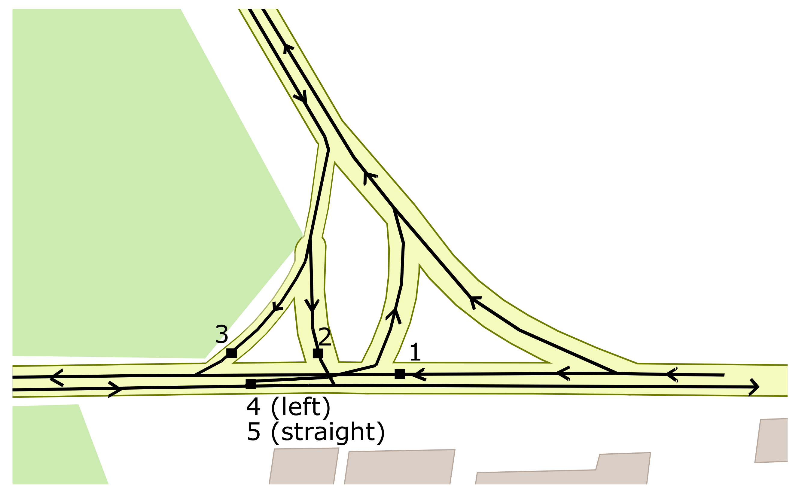
4.1. Case Study, Simulation Scenario and Setup

We consider a real road junction in Rome, Italy (Figure 1). The current TL control cycle implemented at the road junction is as follows:

• TLs 1 and 5 are green for 40 s;
• TL 1 is yellow and TL 5 is green for 5 s;
• TLs 5 and 4 are green for 15 s;
• TLs 5 and 4 are yellow for 5 s;
• TLs 2 and 3 are green for 25 s;
• TLs 2 and 3 are yellow for 5 s, then a new cycle starts.

We simulate three hours of traffic: with low, medium and high vehicle arrival rates, respectively. The vehicle arrival rates follow a Poisson distribution. The average arrival rates ${\lambda }_i$ for the different TL are reported in

Table 1. Car arrival rates at the TLs.

Traffic Intensity	${\mathit{\lambda }}_1$	${\mathit{\lambda }}_2$	${\mathit{\lambda }}_3$	${\mathit{\lambda }}_4$	${\mathit{\lambda }}_5$
Low	0.13	0.086	0.086	0.05	0.2
Medium	0.52	0.35	0.35	0.2	0.8
High	0.975	0.645	0.645	0.375	1.5

(${\lambda }_i$ is the expected number of vehicles arriving at the 5 TLs every T seconds). They reflect a realistic distribution of traffic load on the 5 roads constituting the junction.

Simulations have been performed using the Julia programming language (https://julialang.org/), version 1.3.1 [24]. The quadratic mixed-integer optimization problem constituting the MPC iteration has been modeled using the Julia library JuMP [25] and solved with the Gurobi solver (http://www.gurobi.com/). The simulations have been performed on a Window 10 machine, 64 bit, equipped with an Intel I7-5500U CPU, 2.40 GHz and 8 GB RAM. A sampling time T of 5 seconds, and a value of $N=15$ have been chosen.

4.2. Queue Balancing

A sequence of vehicle arrivals in time at the different TLs is generated according to the arrival rates reported in Table 1. The sequence of vehicles arrivals is shown in Figure 2.

The results of the simulations are reported in Figure 3, Figure 4 and Figure 5. The figures report, respectively, the comparison of the queue lengths at the five TLs, resulting from traditional control (gray line) and MPC control (black line), for the three hours of simulations.

The average queue lengths at the different TLs for the 3 h of test are reported in

Table 2. Average queue length at the TLs. Out of the brackets the values from proposed control, in brackets the ones from traditional control.

Average Queue Length	${\mathit{TL}}_1$	${\mathit{TL}}_2$	${\mathit{TL}}_3$	${\mathit{TL}}_4$	${\mathit{TL}}_5$
Hour 1 (low traffic)	0.47 (0.35)	0.62 (0.58)	0.68 (0.58)	0.37 (0.42)	0.58 (0.34)
Hour 2 (medium)	1.47 (2.34)	1.32 (2.35)	1.02 (2.17)	1.02 (1.60)	1.95 (1.80)
Hour 3 (high)	5.29 (10.44)	7.72 (8.46)	2.54 (7.51)	3.43 (8.60)	6.96 (7.23)

(in brackets the values resulting from traditional control).

By analysing the figures and the table, it can be seen that the proposed MPC controller brings significant improvements under medium and high arrival rates, while the algorithm is not effective under low rates, where simpler reactive strategies are preferable. Notice from Figure 5 how the proposed algorithm manages to reduce and flatten the highest peaks of the queue curves, especially for TLs 1, 3 and 4.

Finally, the solving times for the 2160 MPC iterations (i.e., 3 h of simulation with a sampling time of 5 s) are reported in Figure 6. Solving times are compatible with the sampling time T used.

5. Conclusions

This paper has presented a model predictive control (MPC) approach to the management of a road junction. The MPC algorithm controls the timing of the traffic lights (TLs) governing the road junction. The resulting optimization problem is a quadratic mixed-integer one and the resulting solving times are compatible with real implementation. The results have shown the effectiveness of the algorithm in balancing the queues at the road junction, compared to a classic control strategy where the timing of the TLs are fixed.

In future works, the proposed algorithm will be extended to make it able to more accurately account for the evolution of the cumulative and single vehicles’ waiting times at the TLs, so that waiting times can be better traded off with the balancing of the queue lengths. Another line of research regards the derivation of distributed variants of the proposed MPC algorithm, to tackle the case of multi-junction road networks. Finally, the resulting algorithms will be validated using more advanced and realistic simulation tools (such as Anylogic [26] or SUMO (“Simulation of Urban MObility”) [27]).

References

1. Smith, M.J.; Iryo, T.; Mounce, R.; Rinaldi, M.; Viti, F. Traffic control which maximises network throughput: Some simple examples. Transp. Res. Part C Emerg. Technol. 2019, 107, 211–228. [Google Scholar] [CrossRef]
2. Chow, A.H.; Sha, R.; Li, S. Centralised and decentralised signal timing optimisation approaches for network traffic control. Transp. Res. Part C Emerg. Technol. 2019, 113, 108–123. [Google Scholar] [CrossRef]
3. Małecki, K.; Pietruszka, P.; Iwan, S. Comparative analysis of selected algorithms in the process of optimization of traffic lights. In Asian Conference on Intelligent Information and Database Systems; Springer: Cham, Switzerland, 2017; pp. 497–506. [Google Scholar]
4. Liang, X.; Du, X.; Wang, G.; Han, Z. A deep reinforcement learning network for traffic light cycle control. IEEE Trans. Veh. Technol. 2019, 68, 1243–1253. [Google Scholar] [CrossRef] [Green Version]
5. Bui, K.H.N.; Jung, J.E.; Camacho, D. Game theoretic approach on Real-time decision making for IoT-based traffic light control. Concurr. Comput. Pract. Exp. 2017, 29, e4077. [Google Scholar] [CrossRef]
6. Leal, S.S.; de Almeida, P.E.M.; Chung, E. Active control for traffic lights in regions and corridors: An approach based on evolutionary computation. Transp. Res. Procedia 2017, 25, 1769–1780. [Google Scholar] [CrossRef]
7. Garg, H.; Kaushal, E.G. Traffic Lights Control System for Indian Cities Using WSN and Fuzzy Control. Traffic 2017, 4, 56–65. [Google Scholar]
8. Ye, B.L.; Wu, W.; Ruan, K.; Li, L.; Chen, T.; Gao, H.; Chen, Y. A survey of model predictive control methods for traffic signal control. IEEE/CAA J. Autom. Sin. 2019, 6, 623–640. [Google Scholar] [CrossRef]
9. Kamal, M.; Imura, J.; Hayakawa, T.; Ohata, A.; Aihara, K. Traffic Signal Control in an MPC Framework Using Mixed Integer Programming. IFAC Proc. Vol. 2013, 46, 645–650. [Google Scholar] [CrossRef]
10. Kamal, M.A.S.; Imura, J.i.; Hayakawa, T.; Ohata, A.; Aihara, K. Traffic signal control of a road network using MILP in the MPC framework. Int. J. Intell. Transp. Syst. Res. 2015, 13, 107–118. [Google Scholar] [CrossRef]
11. Jin, S.; Hou, Z.; Chi, R.; Bu, X. Model free adaptive predictive control approach for phase splits of urban traffic network. In Proceedings of the 2016 Chinese Control and Decision Conference (CCDC), Yinchuan, China, 28–30 May 2016; pp. 5750–5754. [Google Scholar]
12. Wang, Q.; Abbas, M. Optimal urban traffic model predictive control for NEMA standards. Transp. Res. Rec. 2019, 2673, 413–424. [Google Scholar] [CrossRef]
13. Eini, R.; Abdelwahed, S. Distributed Model Predictive Control for Intelligent Traffic System. In Proceedings of the 2019 International Conference on Internet of Things (iThings) and IEEE Green Computing and Communications (GreenCom) and IEEE Cyber, Physical and Social Computing (CPSCom) and IEEE Smart Data (SmartData), Atlanta, GA, USA, 14–17 July 2019; pp. 909–915. [Google Scholar]
14. Li, X.; Sun, J.Q. Multi-objective optimal predictive control of signals in urban traffic network. J. Intell. Transp. Syst. 2019, 23, 370–388. [Google Scholar] [CrossRef]
15. Wu, N.; Li, D.; Xi, Y.; de Schutter, B. Distributed Event-Triggered Model Predictive Control for Urban Traffic Lights. IEEE Trans. Intell. Transp. Syst. 2020, 1–11. [Google Scholar] [CrossRef]
16. Glover, F. Improved linear integer programming formulations of nonlinear integer problems. Manag. Sci. 1975, 22, 455–460. [Google Scholar] [CrossRef] [Green Version]
17. Zheng, J.; Liu, H.X. Estimating traffic volumes for signalized intersections using connected vehicle data. Transp. Res. Part C Emerg. Technol. 2017, 79, 347–362. [Google Scholar] [CrossRef] [Green Version]
18. Han, E.; Lee, H.P.; Park, S.; So, J.J.; Yun, I. Optimal signal control algorithm for signalized intersections under a V2I communication environment. J. Adv. Transp. 2019, 2019. [Google Scholar] [CrossRef]
19. Bemporad, A.; Morari, M. Control of systems integrating logic, dynamics, and constraints. Automatica 1999, 35, 407–427. [Google Scholar] [CrossRef]
20. Little, J.D.; Graves, S.C. Little’s law. In Building Intuition: Insights from Basic Operations Management Models and Principles; Springer: Berlin/Heidelberg, Germany, 2008; pp. 81–100. [Google Scholar]
21. Stellato, B.; Naik, V.V.; Bemporad, A.; Goulart, P.; Boyd, S. Embedded mixed-integer quadratic optimization using the OSQP solver. In Proceedings of the 2018 European Control Conference (ECC), Limassol, Cyprus, 12–15 June 2018; pp. 1536–1541. [Google Scholar]
22. Sahinidis, N.V. Mixed-Integer Nonlinear Programming 2018; Springer: Berlin/Heidelberg, Germany, 2019. [Google Scholar]
23. Simon, D.; Löfberg, J. Stability analysis of model predictive controllers using Mixed Integer Linear Programming. In Proceedings of the 2016 IEEE 55th Conference on Decision and Control (CDC), Las Vegas, NV, USA, 12–14 December 2016; pp. 7270–7275. [Google Scholar]
24. Bezanson, J.; Edelman, A.; Karpinski, S.; Shah, V. Julia: A Fresh Approach to Numerical Computing. SIAM Rev. 2017, 59, 65–98. [Google Scholar] [CrossRef] [Green Version]
25. Dunning, I.; Huchette, J.; Lubin, M. JuMP: A Modeling Language for Mathematical Optimization. SIAM Rev. 2017, 59, 295–320. [Google Scholar] [CrossRef]
26. Shamlitskiy, Y.I.; Mironenko, S.; Kovbasa, N.; Bezrukova, N.; Tynchenko, V.; Kukartsev, V. Evaluation of the effectiveness of traffic control algorithms based on a simulation model in the AnyLogic. Phys. Conf. Ser. 2019, 1353, 012101. [Google Scholar] [CrossRef] [Green Version]
27. Lopez, P.A.; Behrisch, M.; Bieker-Walz, L.; Erdmann, J.; Flötteröd, Y.P.; Hilbrich, R.; Lücken, L.; Rummel, J.; Wagner, P.; Wießner, E. Microscopic Traffic Simulation using SUMO. In Proceedings of the 21st IEEE International Conference on Intelligent Transportation Systems, Maui, HI, USA, 4–7 November 2018. [Google Scholar]
Figure 1. Example of a road junction. The black squares indicate TLs (for graphic convenience, one square only is placed for TLs 4 and 5).
Smartcities 03 00041 g001
Figure 2. Vehicles arrivals at the TLs (number of vehicles arriving at every time step).
Smartcities 03 00041 g002
Figure 3. Queue lengths at the five TLs (i.e., n 1 to n 5 ), under low vehicle arrival rates (traditional control in gray line, proposed MPC control in black line).
Smartcities 03 00041 g003
Figure 4. Queue lengths at the five TLs (i.e., n 1 to n 5 ), under medium vehicle arrival rates (traditional control in gray line, proposed MPC control in black line).
Smartcities 03 00041 g004
Figure 5. Queue lengths at the five TLs (i.e., n 1 to n 5 ), under high vehicle arrival rates (traditional control in gray line, proposed MPC control in black line).
Smartcities 03 00041 g005
Figure 6. Solving time of the MPC iterations.
Smartcities 03 00041 g006