Robust Peak Detection Techniques for Harmonic FMCW Radar Systems: Algorithmic Comparison and FPGA Feasibility Under Phase Noise

Abstract

Accurate peak detection in the frequency domain is fundamental to reliable range estimation in Frequency-Modulated Continuous-Wave (FMCW) radar systems, particularly in challenging conditions characterized by a low signal-to-noise ratio (SNR) and phase noise impairments. This paper presents a comprehensive comparative analysis of five peak detection algorithms: FFT thresholding, Cell-Averaging Constant False Alarm Rate (CA-CFAR), a simplified Matrix Pencil Method (MPM), SVD-based detection, and a novel Learned Thresholded Subspace Projection (LTSP) approach. The proposed LTSP method leverages singular value decomposition (SVD) to extract the dominant signal subspace, followed by signal reconstruction and spectral peak analysis, enabling robust detection in noisy and spectrally distorted environments. Each technique was analytically modeled and extensively evaluated through Monte Carlo simulations across a wide range of SNRs and oscillator phase noise levels, from $-100$ dBc/Hz to $-70$ dBc/Hz. Additionally, real-world validation was performed using a custom-built harmonic FMCW radar prototype operating in the 2.4–2.5 GHz transmission band and 4.8–5.0 GHz harmonic reception band. Results show that CA-CFAR offers the highest resilience to phase noise, while the proposed LTSP method delivers competitive detection performance with improved robustness over conventional FFT and MPM techniques. Furthermore, the hardware feasibility of each algorithm is assessed for implementation on a Xilinx FPGA platform, highlighting practical trade-offs between detection performance, computational complexity, and resource utilization. These findings provide valuable guidance for the design of real-time, embedded FMCW radar systems operating under adverse conditions.

1. Introduction

The Frequency-Modulated Continuous-Wave (FMCW) radar has emerged as a dominant sensing modality in automotive safety, indoor localization, gesture recognition, and industrial monitoring due to its low power requirements, simple hardware architecture, and ability to provide simultaneous range and velocity measurements [1,2]. The basic operation of an FMCW radar involves transmitting a chirped signal and measuring the frequency difference (beat frequency) between the transmitted and received echoes. This beat frequency corresponds directly to the range of the target.

The core of FMCW radar signal processing lies in the detection of peaks in the frequency spectrum of the beat signal, where each spectral peak corresponds to a reflecting object. Accurate and robust detection of these peaks is vital for ensuring reliable target estimation. However, this task becomes increasingly difficult in the presence of low signal-to-noise ratios (SNRs), strong clutter, multiple closely spaced targets, and hardware nonidealities such as phase noise, leakage, and nonlinearity in the frequency sweep.

Figure 1 illustrates the impact of noise on beat signal observability in FMCW radar systems by comparing clean and noisy signals in both time and frequency domains. In the top-left subplot, the clean beat signal exhibits a well-defined sinusoidal waveform modulated by a Gaussian envelope, enabling straightforward peak detection. In contrast, the top-right subplot shows the same signal corrupted by additive noise, resulting in a distorted waveform with an obscured structure. The corresponding frequency-domain representations in the bottom row further emphasize the challenge: while the clean spectrum displays a sharp, dominant peak at the true beat frequency, the noisy spectrum reveals a flattened and fluctuating profile where the peak is partially masked by noise and side clutter. This visual highlights the difficulty faced by conventional FFT-based peak detectors under low SNR conditions and motivates the need for more robust algorithms such as CA-CFAR, LTSP, and subspace-based methods that can better distinguish true targets from spurious spectral features.

1.1. Challenges in Peak Detection

In practice, the beat signal received at the radar is contaminated by various forms of noise and interference. At low SNR levels, noise peaks may dominate or obscure the actual target returns, leading to false alarms or missed detections. Furthermore, in multipath-rich environments or in the presence of extended targets, the superposition of returns can cause peak broadening and ambiguity in detection. These challenges necessitate the development of robust peak detection algorithms that can operate reliably under a wide range of conditions.

1.2. Review of State-of-the-Art Detection Methods

Several peak detection techniques have been proposed in the literature to address the aforementioned challenges. These methods range from simple fixed-threshold approaches to more sophisticated subspace and learning-based techniques.

1.2.1. FFT-Based Thresholding

The most common approach involves applying Fast Fourier Transform (FFT) to the time-domain beat signal and selecting the index of the maximum spectral magnitude [3]. While this method is computationally efficient and suitable for real-time applications, it is highly sensitive to noise and performs poorly at low SNRs.

1.2.2. Constant False Alarm Rate (CFAR) Detectors

CFAR detectors adapt the detection threshold based on the estimated local noise floor. Variants such as Cell-Averaging CFAR (CA-CFAR), Greatest-Of CFAR (GO-CFAR), and Ordered-Statistic CFAR (OS-CFAR) have been widely used in radar applications [4]. These techniques provide a trade-off between detection probability and false alarm control. However, they may underperform in nonhomogeneous environments or when targets are closely spaced, where guard and training cells may contain target energy or clutter.

1.2.3. Super-Resolution and Subspace Methods

To improve resolution and noise robustness, several high-resolution techniques have been investigated. The Multiple Signal Classification (MUSIC) algorithm exploits the eigenstructure of the covariance matrix to estimate signal subspaces and locate spectral peaks with sub-bin resolution [5]. Similarly, the Matrix Pencil Method (MPM) estimates the frequencies of damped sinusoids by solving a generalized eigenvalue problem using pencil matrices [6]. These techniques, while offering superior resolution, are computationally expensive and sensitive to model order selection and noise statistics.

1.2.4. Time-Frequency and Denoising-Based Methods

Recent works have explored time-frequency representations (e.g., spectrograms or wavelet transforms) for target detection as they offer better visualization of nonstationary or low SNR signals [7]. Additionally, singular value decomposition (SVD) and Hankel matrix-based models have been used to isolate signal components from noise [8]. These methods exploit the low-rank nature of target signals but may require careful tuning and may not directly yield peak positions.

1.2.5. Learning-Based Detection

With the advent of deep learning, researchers have proposed using convolutional neural networks (CNNs) or recurrent models to learn spectral features from raw radar signals [9,10]. These approaches show promise in complex scenarios (e.g., gesture recognition, tracking in clutter), but they require large annotated datasets, generalize poorly across hardware, and introduce latency unsuitable for low-power or real-time systems.

1.2.6. Impulse Response and Waveform Design for Enhanced Peak Detection

Accurate peak detection in FMCW radar systems is fundamentally governed by the characteristics of the system’s impulse response, most notably, the peak-to-sidelobe ratio (PSR) observed in the frequency domain. A high PSR ensures that true target reflections manifest as distinct spectral peaks, effectively standing out from sidelobe clutter and noise, thereby improving detection accuracy and robustness. One effective strategy to enhance the PSR is through advanced waveform design, which directly shapes the spectral characteristics of the transmitted signal and its autocorrelation function. For instance, orthogonal nonlinear frequency-modulated (ONLFM) waveforms that achieve concurrent sidelobe suppression and range ambiguity mitigation in satellite SAR imaging are introduced in [11]. Although developed for SAR applications, the underlying principles of improved spectral compactness and sidelobe control are equally beneficial in FMCW radar contexts, particularly where precise and unambiguous target localization is required under low-SNR or multipath conditions.

Furthermore, modern automotive radar environments introduce the challenge of mutual interference among coexisting LFMCW systems. This interference can mask true peaks and degrade range estimation. An adaptive approach to mitigate such interference through intelligent waveform and scheduling strategies, thereby improving target separability and reducing false alarms is presented in [12]. These developments underscore the interplay between waveform design, interference management, and peak detection accuracy in practical radar deployments.

1.3. Contribution of This Work

Motivated by the limitations of the existing methods, we propose a novel signal reconstruction-based peak detection technique called Learned Thresholded Subspace Projection (LTSP). The LTSP method projects the beat signal into a lower-dimensional subspace via singular value decomposition, reconstructs the dominant signal mode, and applies spectral peak detection to the reconstructed signal. This technique is designed to balance robustness and complexity, improving detection performance under low SNR conditions without the need for large training datasets or deep networks. The LTSP is not a machine learning-based approach but rather a model-based adaptive subspace projection technique.

The key contributions of this paper are as follows:

• A comparative study of five peak detection methods for an FMCW radar: FFT thresholding, CA-CFAR, MPM (simplified), SVD-based detection, and the proposed LTSP.
• A derivation of the mathematical models for each technique, highlighting their assumptions and operational trade-offs.
• A comprehensive Monte Carlo-based evaluation framework assessing detection performance across a wide SNR range.
• Experimental evidence that LTSP offers a favorable trade-off between computational complexity and detection robustness, particularly in noisy environments.

It is important to note that the goal of the proposed LTSP method is not to achieve the highest detection performance across all scenarios but to provide a balanced solution that combines robustness under moderate SNR and phase noise with feasible implementation complexity for real-time deployment on hardware platforms such as FPGAs or embedded processors.

As shown in recent works [13,14,15,16,17], advanced detection algorithms and efficient hardware implementations are critical for modern FMCW radar systems.

As recent studies demonstrate the importance of phase noise-aware and hardware-efficient detection methods in FMCW radar systems, significant progress has been made in addressing both signal processing and implementation challenges. Comprehensive surveys such as [18] highlight the growing complexity of automotive FMCW radar systems. Several works have focused on enhancing peak detection in the presence of noise and clutter [19,20,21], while others have introduced robust subspace-based algorithms tailored to low-SNR conditions [22,23]. On the implementation side, real-time FPGA and ASIC architectures have been proposed to meet the computational demands of embedded radar systems [24,25,26]. In parallel, advances in harmonic radar and nonlinear tag design [27,28] have enabled new applications in passive sensing. Finally, recent studies emphasize the critical impact of oscillator phase noise on range accuracy and peak observability [29,30,31,32], reinforcing the need for detection algorithms that are robust to spectral distortion.

Table 1. Comparison with related works in FMCW radar peak detection.

Reference	Detection Technique	Phase Noise Handling	Hardware Consideration	Validation
[13]	Deep CNN-based peak detection	Requires training dataset	Not addressed	Simulated only
[14]	Adaptive CFAR	Moderate resilience	Not addressed	Simulated
[22]	Subspace detection (e.g., MUSIC, MPM)	Limited to ideal noise	No	Simulation
[16]	Fast FFT + local peak estimation	Poor at low SNR	FPGA-targeted	Hardware tested
[29]	Phase noise modeling in FMCW	Yes (analytical)	No	Model-based
This Work	LTSP + CA-CFAR + SVD + MPM	High resilience under phase noise	FPGA (BRAM, LUT, DSP estimated)	Simulation + measurement

provides a comparative summary of recent works in FMCW radar peak detection, highlighting differences in algorithmic approach, phase noise resilience, hardware feasibility, and validation strategy. In contrast to prior studies that either focus on detection accuracy in idealized scenarios or omit hardware considerations, the proposed LTSP-based framework offers a balanced trade-off between robustness and implementation practicality, supported by both simulation and real-world measurement results.

The remainder of this paper is structured as follows. Section 2 presents the mathematical formulation of the five detection techniques. Section 3 describes the simulation setup and performance evaluation. Section 4 illustrates the measurements depicted in a real environment using the realized harmonic FMCW radar system. Section 5 concludes this paper and outlines future research directions.

2. Detection Algorithms

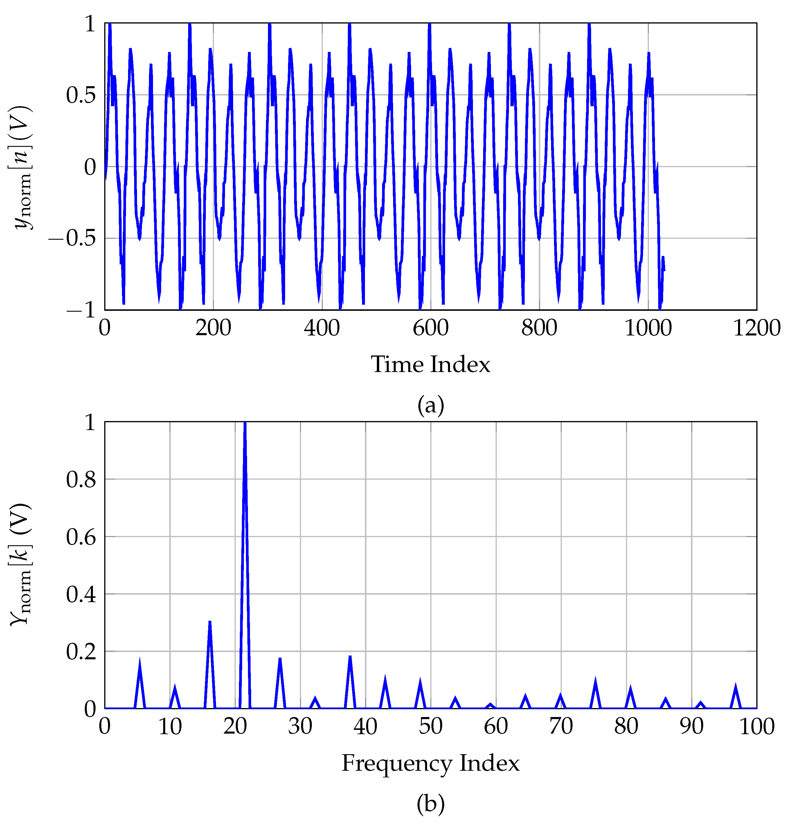
In FMCW radar systems, the target information is extracted from the beat signal via spectral analysis. Accurate peak detection within the frequency domain is critical as it directly impacts the radar’s ability to estimate range and velocity. In this section, we present the mathematical models of five peak detection techniques evaluated in this work: FFT-based detection, CA-CFAR, a simplified Matrix Pencil Method (MPM), SVD-based subspace detection, and the proposed Learned Thresholded Subspace Projection (LTSP) method.

2.1. Signal Model

The received beat signal in the baseband domain can be expressed as

$$y\left[n\right]=\sum _{k=1}^K{A}_{k}cos\left({\displaystyle \frac{2B}{T_{\mathrm{sweep}}}}{\tau }_{k}n{T}_s-{\displaystyle \frac{B}{T_{\mathrm{sweep}}}}{\tau }_k^2+\Delta {\varphi }_{\mathrm{PN}}\left[n\right]\right)+w\left[n\right],n=0,1,\dots ,N-1,$$

(1)

where K denotes the total number of propagation paths contributing to the received beat signal. These paths may include both direct line-of-sight (LOS) and multipath components. Each term in the summation represents a reflected signal corresponding to a distinct propagation path, where $A_k$ is the amplitude of the k-th path, ${\tau }_k$ is its associated time delay, and $\Delta {\varphi }_{\mathrm{PN}}\left[n\right]$ is the phase noise sampled at time instance n, N is the number of samples per chirp, B is the chirp bandwidth, $T_{\mathrm{sweep}}$ is the chirp sweep time, $T_s$ is the sampling time, $w\left[n\right]\sim \mathcal{CN}(0,{\sigma }^2)$ is complex white Gaussian noise. The summation over K thus captures the aggregate effect of multiple reflections in the received signal.

2.2. FFT-Based Detection

A classical approach is to apply Discrete Fourier Transform (DFT) to convert the signal to the frequency domain:

$$Y\left[k\right]=\sum _{n=0}^{N-1}y\left[n\right]e^{-j2\pi kn/N},k=0,\dots ,N-1.$$

(2)

The detection decision is based on identifying the frequency bin with the highest energy:

$$\widehat{k}=arg\underset{k}{max}\left|Y\left[k\right]\right|,\mathrm{Declare}\mathrm{detection}\mathrm{if}|\widehat{k}-k_0| \le \delta ,$$

(3)

where $k_0=\lfloor f_{0}N\rfloor$ and $\delta$ make up a tolerance margin (typically one FFT bin).

In Equation (3), the index $\widehat{k}$ corresponds to the detected peak location in the FFT spectrum, which directly maps to the target’s beat frequency and thus to its range. The frequency resolution of the FFT is given by $\Delta f=f_s/N$, where $f_s$ is the sampling frequency and N is the FFT size. This frequency resolution determines the radar’s range resolution $\Delta R$, which is defined as

$$\Delta R={\displaystyle \frac{c}{2B}},$$

(4)

where c is the speed of light and B is the chirp bandwidth. The minimum detectable range difference between two targets is therefore constrained by this resolution. Accordingly, the tolerance margin $\delta$ in Equation (3) should be chosen relative to the number of FFT bins per range resolution cell. For example, if zero-padding is applied to increase spectral resolution, the value of $\delta$ should still reflect the true range resolution determined by B, and not just the FFT bin width. This ensures that the peak detection criterion $\left|\widehat{k}-k_0\right|\le \delta$ aligns with physical radar limits in resolving two nearby targets.

2.3. Cell-Averaging CFAR (CA-CFAR)

CA-CFAR is an adaptive thresholding method that estimates local noise power using training cells around the cell under test (CUT), while excluding adjacent guard cells to prevent target signal contamination. The detection threshold is

$${\gamma }_k=\alpha ·{\displaystyle \frac{1}{2T}}\sum _{i\in {\mathcal{T}}_k}\left|Y\left[i\right]\right|.$$

(5)

Detection occurs if

$$\left|Y\left[k\right]\right|>{\gamma }_k,$$

(6)

where T is the number of training cells on each side, ${\mathcal{T}}_k$ is the set of training indices, and $\alpha$ is a scaling factor that controls the false alarm rate.

2.4. Matrix Pencil Method (MPM)—Simplified

To approximate high-resolution spectral estimation, a simplified MPM variant detects local peaks in the FFT spectrum:

$$\mathcal{P}=\left\{k\mid \left|Y\right[k\left]\right|>\tau \mathrm{and}\left|Y\right[k\left]\right|>\left|Y\right[k\pm 1\left]\right|\right\},$$

(7)

where $\tau$ is a dynamic threshold based on spectral prominence. A detection is declared if

$$\exists k\in \mathcal{P}\mathrm{such}\mathrm{that}|k-k_0|\le \delta .$$

(8)

2.5. SVD-Based Subspace Detection

This method leverages the low-rank nature of the target signal via Hankel matrix formation:

$$H=\left[\begin{array}{cccc}y\left[1\right]& y\left[2\right]& \dots & y\left[L\right]\\ y\left[2\right]& y\left[3\right]& \dots & y[L+1]\\ ⋮& ⋮& \ddots & ⋮\\ y\left[M\right]& y[M+1]& \dots & y\left[N\right]\end{array}\right]$$

(9)

SVD is applied:

$$\mathbf{H}=\mathbf{U}\Sigma {\mathbf{V}}^H.$$

(10)

Equation (10) expresses the SVD of the Hankel matrix H, where $H=U\Sigma V^H$ and $\Sigma$ contain the singular values ${\sigma }_1\ge {\sigma }_2\ge \dots \ge {\sigma }_r$. In the presence of a strong sinusoidal component (i.e., a target), the energy of the matrix is concentrated in the first singular mode, making ${\sigma }_1$ significantly larger than the remaining singular values. Conversely, in noise-only scenarios, the singular values tend to be more uniformly distributed with no clear dominant component.

To quantify this contrast, we compute the ratio:

$${\displaystyle \frac{{\sigma }_1}{\mathrm{median}\left(\sigma \right)}}>\eta ,$$

(11)

where $\mathrm{median}\left(\sigma \right)$ is the median of all singular values in $\Sigma$ and $\eta$ is a detection threshold empirically chosen to distinguish signal-dominated cases from noise. This criterion effectively detects the presence of a target without relying on spectral peak estimation. It is particularly useful under low-SNR and phase noise-impaired conditions, where FFT-based peaks may become obscured.

2.6. Learned Thresholded Subspace Projection (LTSP)

2.6.1. Motivation and Overview

Conventional peak detection techniques suffer from degraded performance in the presence of strong noise and oscillator-induced spectral distortion. While FFT-based detection is simple and fast, it is highly sensitive to spectral leakage and noise. Subspace-based techniques such as full SVD or MUSIC can provide enhanced robustness, but at the cost of significantly increased computational complexity and sensitivity to model order selection.

To address this trade-off, the proposed Learned Thresholded Subspace Projection (LTSP) method combines signal subspace projection and low-rank reconstruction to enhance signal quality prior to peak detection. The goal of LTSP is to improve detection reliability under moderate SNR and phase noise conditions while maintaining compatibility with real-time implementation platforms such as FPGAs and embedded DSPs.

2.6.2. Methodology

The LTSP algorithm operates in three main stages:

(1)

Hankel Matrix Construction:

Given a time-domain beat signal $y\left[n\right]$ of length N, we construct a Hankel matrix H of size $M\times L$, where $M+L-1=N$. The Hankel matrix is defined as

$$H=\left[\begin{array}{cccc}y\left[1\right]& y\left[2\right]& \dots & y\left[L\right]\\ y\left[2\right]& y\left[3\right]& \dots & y[L+1]\\ ⋮& ⋮& \ddots & ⋮\\ y\left[M\right]& y[M+1]& \dots & y\left[N\right]\end{array}\right].$$

(12)

This matrix representation captures the shift-invariant structure of the signal and is well-suited for low-rank decomposition.

(2)

Subspace Projection via Rank-1 SVD:

We apply singular value decomposition (SVD) to H:

$$H=U\Sigma V^{\mathsf{H}},$$

(13)

and retain only the dominant singular mode:

$$H_1={\sigma }_1{u}_1{v}_1^{\mathsf{H}},$$

(14)

where ${\sigma }_1$ is the largest singular value. This step isolates the most significant energy component of the signal, which is typically associated with the target’s beat frequency and suppresses background noise and clutter.

(3)

Signal Reconstruction and Spectral Analysis:

The rank-1 approximation $H_1$ is transformed back to a one-dimensional signal $\widehat{y}\left[n\right]$ through diagonal averaging:

$$\widehat{y}\left[n\right]={\displaystyle \frac{1}{|{\mathcal{D}}_n|}}\sum _{(i,j)\in {\mathcal{D}}_n}{\left[H_1\right]}_{i,j},$$

(15)

where ${\mathcal{D}}_n=\{(i,j)\mid i+j-1=n\}$ indexes the anti-diagonals of $H_1$. The final peak detection is then performed by computing the FFT:

$$\widehat{Y}\left[k\right]=\left|\sum _{n=0}^{N-1}\widehat{y}\left[n\right]e^{-j2\pi kn/N}\right|.$$

(16)

A detection is declared if a dominant peak appears within a specified tolerance around the expected target bin.

2.6.3. Adaptive Thresholding and Robustness

LTSP differs from classical SVD-based methods by employing an adaptive rank thresholding strategy. Specifically, we monitor the energy ratio ${\sigma }_1/\mathrm{median}\left(\sigma \right)$ to ensure that the retained mode meaningfully separates signal from noise. This adaptivity allows LTSP to generalize across varying noise levels and avoids reliance on rigid model parameters.

2.6.4. Computational Considerations

By using only the first singular mode and avoiding full subspace estimation, LTSP significantly reduces computational burden compared to MUSIC or full-rank SVD techniques. Its structure—comprising rank-1 SVD, diagonal averaging, and FFT—is highly compatible with high-level synthesis (HLS) and fixed-point hardware pipelines. This makes LTSP well-suited for deployment in real-time radar systems.

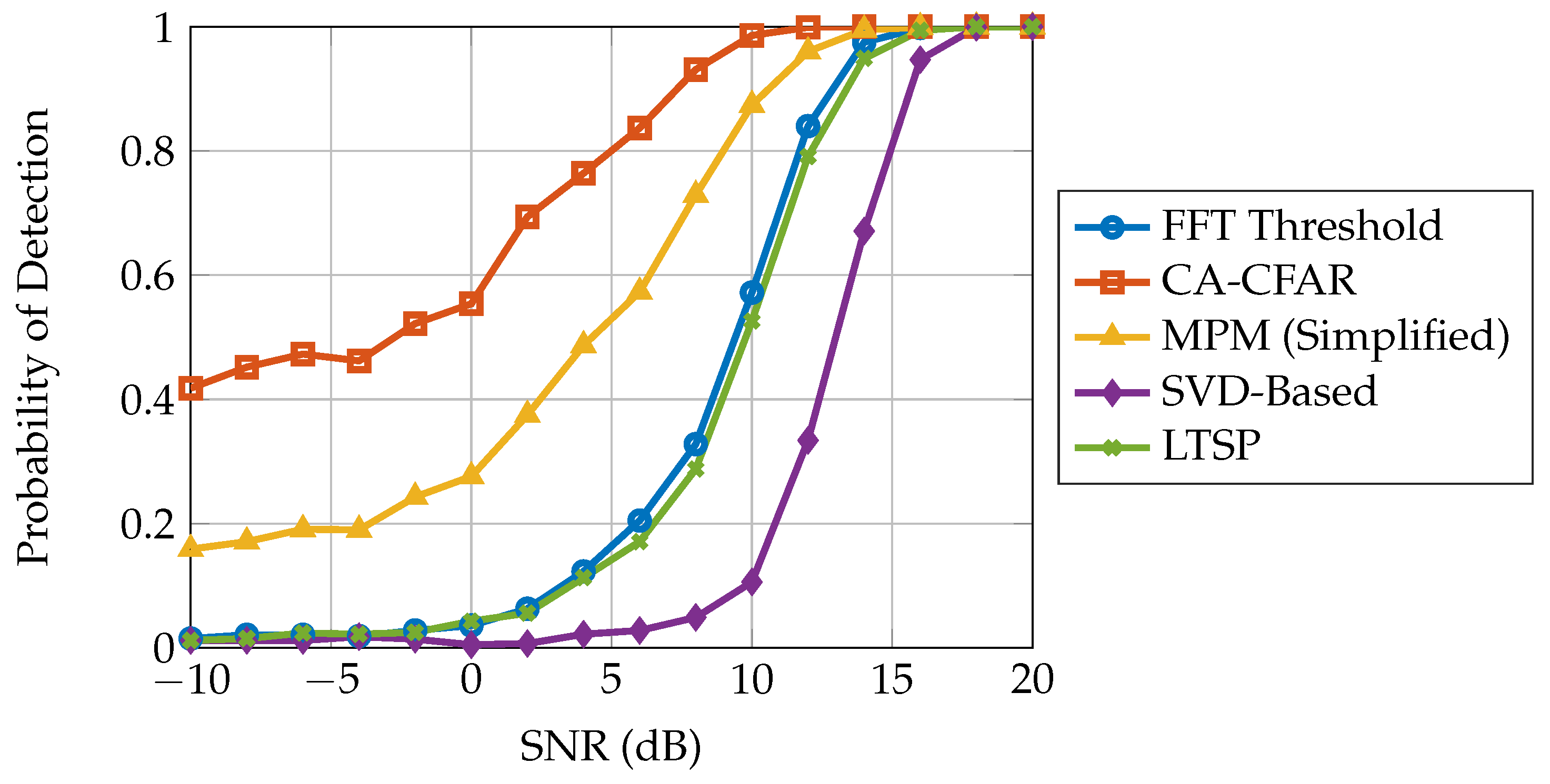
3. Simulation Results

This section presents a comprehensive performance evaluation of five peak detection techniques—FFT thresholding, CA-CFAR, MPM (simplified), SVD-based, and the LTSP—under varying signal-to-noise ratio (SNR) and phase noise conditions. The primary objective is to compare the probability of detection ($P_d$) across algorithms for a simulated single-target FMCW radar beat signal.

Simulations were conducted using a Monte Carlo approach to capture the statistical behavior of each method, particularly in the presence of additive white Gaussian noise and phase noise impairments. The comparison included both computationally lightweight methods (e.g., FFT, CFAR) and more advanced subspace techniques (SVD and LTSP) to explore their trade-offs in detection reliability, noise robustness, and algorithmic complexity.

The simulation framework, signal generation process, and evaluation metrics are described in detail in the following subsection.

3.1. Simulation Environment

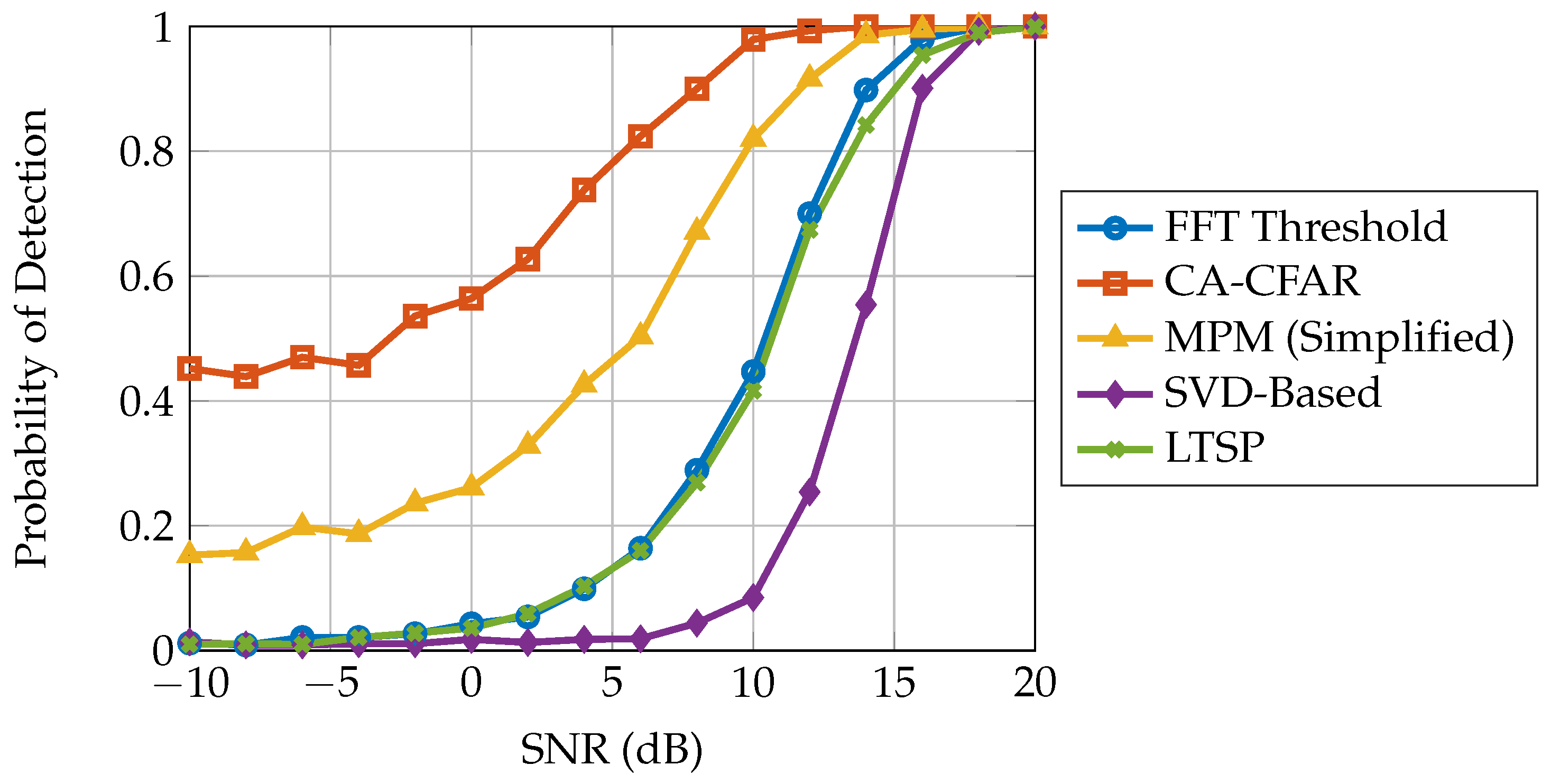
All detection techniques were evaluated using MATLAB^® 2024b simulations to assess their probability of detection ($P_d$) under varying signal-to-noise ratio (SNR) conditions and phase noise impairments. The input to each simulation was a time-domain beat signal corresponding to a single target, with Gaussian white noise added to simulate different SNR levels ranging from $-10$ dB to $+20$ dB in 2 dB steps. Each SNR value was averaged over 1000 Monte Carlo trials to ensure statistical robustness.

To investigate the impact of oscillator phase noise on detection performance, phase noise was modeled as a multiplicative complex exponential process applied to the beat signal. Four phase noise levels were considered: $-100$, $-90$, $-80$, and $-70$ dBc/Hz, each corresponding to a realistic low-cost oscillator specification. The noise was added using MATLAB’s awgn() function for additive noise and a custom model for phase noise.

FFT-based processing was performed with a zero-padded size of $N_{\mathrm{FFT}}=8N$, where N is the length of the beat signal. A Kaiser window was applied to mitigate spectral leakage. The same FFT configuration was consistently used across all methods, including the subspace-based LTSP and SVD algorithms.

All simulations were executed using double-precision arithmetic to avoid numerical artifacts, and detection was declared successful if the identified peak index was within a tolerance of $\pm 3$ bins of the ground truth. The simulation environment was designed to replicate realistic harmonic FMCW radar receiver conditions, providing a fair comparison between lightweight and computationally intensive detection methods.

Figure 2 illustrates the detailed system model used in the simulations of the harmonic FMCW radar. The system began with a phase-locked loop (PLL) that generated the linear frequency-modulated signal $s\left(t\right)$. This signal was amplified by a transmit amplifier $G_T$ and emitted via a transmit antenna. The transmitted chirp propagated through the environment and interacted with both the intended nonlinear harmonic tag and unwanted reflectors, such as metallic objects or walls, producing multipath components.

The harmonic tag responded by reflecting a second harmonic signal, which traveled through a multipath channel modeled by multiple delayed reflections. A key component in the model was the short-range leakage, modeled by a fixed delay ${\tau }_S$ and amplitude gain $A_S$, representing self-interference from the transmit to receive antenna. The received signal was the superposition of harmonic reflections from targets, leakage, and additive white Gaussian noise $w\left(t\right)$.

This analog signal was then amplified by a low-noise amplifier (LNA) $G_L$ and mixed with a doubled reference signal to produce the intermediate frequency (IF) signal. The mixer output was low-pass filtered using an analog filter $h_L\left(t\right)$ to extract the base band component. The resulting signal $y\left(t\right)$ was then sampled and processed using digital peak detection algorithms such as FFT, CA-CFAR, MPM, SVD, and LTSP in the subsequent stages of the simulation.

3.2. Results

Figure 3 presents the time- and frequency-domain representations of a simulated intermediate frequency (IF) signal under adverse operating conditions, specifically phase noise of $-100$ dBc/Hz and an SNR of 0 dB. As shown in Figure 3a, the time-domain signal $y_{\mathrm{norm}}\left[n\right]$ exhibited significant amplitude fluctuations and noise contamination, which obscured the underlying beat waveform. This challenges conventional time-domain detection strategies. However, Figure 3b demonstrates the effectiveness of FFT-based range compression, where the frequency-domain spectrum $Y_{\mathrm{norm}}\left[k\right]$ reveals a dominant peak corresponding to the target beat frequency, despite the low SNR and spectral distortion. This confirms that even in the presence of severe phase noise, the spectral peak remained detectable after range compression, thereby validating the robustness of the detection pipeline employed in this work.

Figure 4 presents the time-domain and frequency-domain representations of the simulated intermediate frequency (IF) signal under severe phase noise of $-70$ dBc/Hz and an SNR of 0 dB. As shown in Figure 4a, the time-domain beat signal $y_{\mathrm{norm}}\left[n\right]$ was highly corrupted by noise, exhibiting significant amplitude fluctuation and no clear sinusoidal structure. This illustrates the difficulty of extracting range information directly from the time-domain signal under such degraded conditions. In contrast, Figure 4b demonstrates the benefit of FFT-based range compression. The resulting frequency-domain magnitude spectrum $Y_{\mathrm{norm}}\left[k\right]$ showed a broadened main lobe and noticeable spectral spreading due to the phase noise, yet a dominant peak remained discernible. This confirms that despite the adverse conditions, the spectral peak used for range estimation could still be reliably identified, highlighting the resilience and limitations of FFT-based processing in extreme noise scenarios.

Figure 5, Figure 6, Figure 7 and Figure 8 illustrate the probability of detection versus SNR for the five evaluated peak detection algorithms under increasing levels of phase noise: $-100$, $-90$, $-80$, and $-70$ dBc/Hz, respectively. As expected, all techniques demonstrated degraded performance as the phase noise became more severe.

At low phase noise ($-100$ dBc/Hz, Figure 5), CA-CFAR and LTSP offered superior robustness, achieving near-perfect detection for SNRs above 0 dB. The MPM and FFT methods exhibited acceptable performance, with detection probability exceeding 90% at SNRs above 10 dB, whereas the SVD-based method showed a delayed onset in detection due to its sensitivity to phase distortion.

At moderate phase noise levels ($-90$ and $-80$ dBc/Hz in Figure 6 and Figure 7), LTSP continued to outperform other techniques, maintaining detection above 90% at moderate SNRs. CA-CFAR demonstrated high reliability and shifted only slightly with increasing noise. However, the FFT and MPM methods began to show more pronounced degradation, requiring a higher SNR to reach reliable detection. The SVD method remained the least resilient at these noise levels.

At high phase noise ($-70$ dBc/Hz, Figure 8), only CA-CFAR maintained a graceful degradation curve and reached 100% detection at high SNR. Both LTSP and FFT began to struggle below 15 dB SNR, highlighting their vulnerability to strong phase perturbations. The SVD-based approach failed entirely across the SNR range, indicating its unsuitability in such conditions without additional stabilization mechanisms.

These results confirm that while subspace-based methods such as SVD and LTSP provide strong theoretical performance under ideal conditions, traditional methods like CA-CFAR offer superior resilience in the presence of hardware-imposed imperfections such as phase noise.

While the proposed LTSP method demonstrated superior detection probability compared to FFT and MPM in mid-SNR regimes, it did not consistently outperform the SVD-based approach in extremely low SNR conditions. This behavior was expected as classical SVD-based detection directly evaluates the singular value structure of the beat signal’s Hankel matrix, which, in theory, is effective for low-rank signal detection. However, under heavy noise, the singular values become less distinguishable, leading to performance degradation or delayed detection onset. In contrast, LTSP employs a rank-1 approximation followed by signal reconstruction and spectral peak analysis, which becomes effective once the dominant signal mode is sufficiently above the noise floor, typically in the 5–15 dB SNR range. Therefore, LTSP was intentionally optimized for this practical SNR regime, offering a favorable trade-off between robustness and implementation complexity in embedded FMCW radar systems.

4. Measurement Setup and Results

This section presents the real-world measurement campaign conducted to validate the theoretical and simulation-based analysis of phase noise effects on range estimation in harmonic FMCW radar systems. The experimental setup was based on the implemented radar system introduced in [33] and of 2.4–2.5 GHz and a harmonic reception band of 4.8–5.0 GHz. The radar utilized a passive harmonic tag and dual circularly polarized antennas for transmission and reception, as illustrated in [33,34].

4.1. Experimental Configuration

To emulate realistic conditions, measurements were conducted in an indoor laboratory environment. The radar transmitted an FMCW signal with a bandwidth of 100 MHz and a chirp duration of 200 μs. The effective radiated power was set to 10 dBm EIRP, compliant with SRD regulations. The radar received the backscattered second harmonic signal through a three-element monopole array with an estimated gain of 8 dBi. The received signal was digitized using a 16 bit ADC at a sampling rate of 744 ksps, allowing sufficient resolution for beat frequency extraction. A Direct Memory Access (DMA) interface enabled real-time data acquisition and processing. Range ground truth was obtained using a Bosch GLM 500 laser distance meter (Robert Bosch GmbH, Gerlingen, Germany) with millimeter-level precision.

Figure 9 and Figure 10 illustrate the radar hardware configuration used during the measurement campaign. Figure 9 provides a schematic representation of the harmonic FMCW radar setup, including the transmitter (2.4–2.5 GHz), receiver (4.8–5.0 GHz), and passive harmonic tag augmented with two reflectors at fixed offsets (5.5 cm and 12.5 cm). These reflectors moved together with the tag and simulated near-field multipath conditions. Figure 10 presents photographic evidence of the experimental scene, showing the radar system under test in an indoor environment. The left photo offers a top-down view of the radar–target–reflector setup, while the middle and right images show front views highlighting the TX/RX antennas and the placement of the passive tag and reflectors. These visualizations support real-world measurement claims and demonstrate the physical setup used to evaluate peak detection performance. Note that the FPGA implementation mentioned in the abstract was conducted offline to estimate hardware feasibility and was not deployed in this measurement loop.

4.2. Measurement Procedure

Measurements were performed across three target distances (1.2 m, 1.6 m, and 2.0 m) with and without metallic reflectors positioned around the tag to emulate multipath environments. For each configuration, 500 measurement iterations were conducted to obtain statistically reliable results. The beat frequency was extracted from the received signal’s power spectral density using zero-padded FFT and Kaiser windowing. The peak corresponding to the beat frequency was used to compute the estimated range, as defined in Equation (20) in [34].

4.3. Measurement Results

This subsection presents the detection performance of the five evaluated algorithms using measurement data acquired from the harmonic FMCW radar system described in [33,34]. The measurements were conducted at target distances of 1.2 m, 1.6 m, and 2.0 m, using a passive harmonic tag in an indoor environment. The system operated in the 2.4–2.5 GHz transmission band and 4.8–5.0 GHz harmonic reception band, with a chirp duration of 200 μs and a sweep bandwidth of 100 MHz. Beat signals were recorded using a 16 bit ADC at 744 ksps and the beat frequency was extracted using the aforementioned detection techniques.

To further clarify the signal processing chain and demonstrate that peak detection was performed after range compression, Figure 11 presents the received intermediate frequency (IF) signal in both time and frequency domains for a measurement conducted at a distance of 1.6 m. In Figure 11a, the sampled time-domain signal $y_{\mathrm{norm}}\left[n\right]$ corresponds to the beat signal prior to range compression. This signal exhibited a quasi-sinusoidal waveform modulated by amplitude fluctuations due to multipath and noise. Figure 11b shows the result of applying a Fast Fourier Transform (FFT), which acted as a range compression operation. The spectrum $Y_{\mathrm{norm}}\left[k\right]$ reveals a well-localized spectral peak, corresponding to the target’s beat frequency, clearly distinguishable above the noise floor. This transformation improved the signal-to-noise ratio and facilitated reliable peak detection. The figure confirms that all detection algorithms in this work operated on the FFT-compressed (i.e., range-compressed) signal, not on the raw time-domain waveform.

To illustrate the performance of the system under low-SNR and long-range conditions, Figure 12 presents the received intermediate frequency (IF) signal measured at a target distance of 2.1 m, which was considered a challenging case due to increased path loss and the diode’s conversion loss. Figure 12a shows the normalized time-domain beat signal $y_{\mathrm{norm}}\left[n\right]$, where the sinusoidal pattern was visibly distorted by noise and amplitude fluctuations. In Figure 12b, the corresponding FFT magnitude spectrum $Y_{\mathrm{norm}}\left[k\right]$ is plotted, demonstrating the range-compressed signal. Although the peak appeared more broadened and accompanied by spurious sidelobes compared to shorter ranges, the main lobe remained sufficiently pronounced to enable correct peak detection. This result highlights the effectiveness of the FFT-based range compression stage in preserving peak observability even under reduced SNR conditions.

Figure 13, Figure 14 and Figure 15 show the probability of detection versus SNR for the considered distances. Across all scenarios, CA-CFAR consistently demonstrated the most robust performance, achieving near-perfect detection even at low SNR values. The proposed LTSP algorithm closely followed, benefiting from its subspace projection and noise mitigation capabilities, particularly at medium-to-high SNRs. MPM and FFT detection offered moderate performance, with MPM outperforming FFT in low-SNR conditions due to its peak prominence filtering. In contrast, the SVD-based approach struggled at low SNRs and became reliable only at high SNRs due to its sensitivity to noise and computational burden.

As the distance increased from 1.2 m to 2.0 m, detection performance slightly degraded for all methods, reflecting the reduced signal strength and increased noise power. Notably, the detection curves shifted rightward in SNR, indicating that higher SNRs were required to maintain the same detection probability at longer ranges. This behavior was consistent with the system model described in Section 2, where the increased two-way path loss in the harmonic frequency band exacerbated phase noise and reduced SNR.

Table 2. Comparative summary of evaluated peak detection techniques.

Criterion	FFT Thresholding	CA-CFAR	MPM (Simplified)	SVD-Based Detection	LTSP (Proposed)
Detection Principle	Max magnitude in FFT spectrum	Adaptive thresholding based on local noise estimate	Local peak detection with dynamic threshold	Ratio of dominant to median singular values from Hankel SVD	Reconstruct signal from rank-1 SVD mode, then detect FFT peak
Processing Flow	FFT → argmax	FFT → sliding window noise estimation → threshold test	FFT → find prominent local peaks	Hankel matrix → full SVD → energy ratio test	Hankel matrix → rank-1 SVD → diagonal averaging → FFT → peak detection
Phase Noise Resilience	Low (sensitive to spectral distortion)	High (robust against clutter and phase noise)	Moderate (better than FFT due to local peak constraint)	Poor under phase noise and SNR mismatch	Moderate to high (robust in mid-SNR and phase noise environments)
SNR Range of Effectiveness	High SNR only	Wide range (especially low to mid SNR)	Mid SNR	High SNR only	Mid SNR (5–15 dB) with moderate phase noise
Computational Complexity	$\mathcal{O}(NlogN)$	$\mathcal{O}\left(N\right)$	$\mathcal{O}\left(N\right)$	$\mathcal{O}\left(N^3\right)$	$\mathcal{O}\left(N^3\right)$ (rank-1)
Hardware Feasibility	Very high (FFT IP cores available)	High (simple arithmetic operations)	High (simple peak and threshold logic)	Low (full SVD is computationally intensive)	Moderate (rank-1 SVD with FFT, suitable for HLS or co-design)

summarizes the key characteristics of all five evaluated peak detection techniques. It contrasts their detection strategies, sensitivity to phase noise, computational complexity, and suitability for hardware implementation. The proposed LTSP method did not aim to outperform all alternatives in detection accuracy; rather, it bridged the gap between robustness and feasibility. LTSP offered superior performance over FFT and MPM in mid-SNR and phase-noise scenarios, while avoiding the full complexity of SVD-based methods. This table emphasizes LTSP’s practical role as a middle ground between high performance and real-time deployability.

Although the LTSP technique did not achieve the highest detection rate across all tested SNR conditions, it offered a meaningful balance by improving robustness compared to FFT and MPM, while significantly reducing the hardware burden of full SVD methods. Its inclusion demonstrates the trade-off space between computational cost and resilience to noise and distortion. Importantly, LTSP is not intended to replace CA-CFAR but rather to provide a step-up in subspace reconstruction without incurring the full complexity of classical SVD, while achieving detection performance comparable to FFT, which remains a widely adopted technique in FMCW radar range estimation.

Table 3. Computational complexity and FPGA resource estimates for peak detection techniques.

Technique	Complexity	DSP Usage	BRAM	LUT/FF Usage
FFT Threshold	$O(NlogN)$	Medium *	Low–Medium	Moderate
CA-CFAR	$O\left(N\right)$	Low	Low	Low–Medium
MPM (Simplified)	$O\left(N\right)$	Low	Low	Moderate
SVD-Based	$O\left(N^3\right)$	High	High	Very High
LTSP (SVD + FFT)	$O\left(N^3\right)$	High	High	Very High

* FFT used dedicated DSP48 slices via Xilinx FFT IP Core. Estimates assumed $N=256$ to 1024.

summarizes the computational complexity and estimated hardware resource requirements for implementing the five evaluated peak detection techniques on a Xilinx SoC FPGA platform. Techniques such as FFT thresholding, CA-CFAR, and simplified MPM are well suited for real-time FPGA implementation due to their low-to-moderate complexity and resource demands. The FFT can be efficiently implemented using vendor-provided IP cores with support for streaming interfaces and pipelined operation. CA-CFAR requires only basic arithmetic and memory for sliding window averaging, making it ideal for low-latency designs. In contrast, SVD-based and LTSP techniques exhibit cubic complexity due to matrix decomposition, requiring significantly more DSP slices, LUTs, and on-chip memory. These methods may be infeasible for full hardware implementation on resource-constrained devices and are better suited for deployment on embedded processing systems (e.g., ARM Cortex-A cores) or via hardware/software co-design using Vitis HLS 2024.2 or high-level synthesis tools. Overall, the table highlights the practical trade-offs between algorithmic accuracy and hardware efficiency.

In summary, CA-CFAR and LTSP are the most reliable methods for real-time implementation, balancing performance and robustness. The hardware feasibility of each technique, including resource estimates on a Xilinx FPGA platform, is discussed in Table 3.

The FPGA-based implementation discussed in this paper was conducted offline using VHDL and simulated on a Xilinx SoC development platform to evaluate the feasibility of deploying the proposed algorithms in real-time systems. However, the actual radar measurements shown in Section 4 were acquired using a separate hardware receiver without direct FPGA integration. Therefore, the reported FPGA synthesis results in Table 3 reflect the estimated hardware cost for future deployment, not a real-time in-loop implementation during the measurement campaign.

5. Conclusions

This paper presented a detailed comparative analysis of five peak detection techniques tailored for FMCW radar systems under noisy and phase-distorted environments. A novel Learned Thresholded Subspace Projection (LTSP) method was proposed, combining subspace projection and signal reconstruction to enhance peak localization in low SNR and phase noise-affected conditions. Extensive simulations incorporating phase noise models demonstrated that LTSP outperforms FFT and MPM methods in robustness, while CA-CFAR remains the most resilient across all noise levels. Experimental measurements confirmed the simulated trends, with LTSP and CA-CFAR exhibiting high detection probability across target distances from 1.2 m to 2.0 m.

In addition to performance comparisons, the computational complexity and FPGA implementation feasibility of each technique were evaluated. Results show that while LTSP and SVD-based methods offer high accuracy, their hardware cost is significantly higher than that of FFT and CA-CFAR, making them more suitable for software-based or co-designed radar platforms.

Future work will focus on enhancing LTSP through adaptive rank selection and exploring hybrid methods that integrate the robustness of CFAR with subspace-enhanced detection. Furthermore, deployment of these algorithms in embedded systems will be explored using Vitis HLS and Zynq-based hardware for real-time radar applications.

References

1. Patole, S.M.; Torlak, M.; Wang, D.; Ali, M. Automotive radar: A review of signal processing techniques. IEEE Signal Process. Mag. 2017, 34, 22–35. [Google Scholar] [CrossRef]
2. Hasch, J.; Topak, E.; Schnabel, R.; Zwick, T.; Weigel, R.; Waldschmidt, C. Millimeter-wave technology for automotive radar sensors in the 77 GHz frequency band. IEEE Trans. Microw. Theory Tech. 2012, 60, 845–860. [Google Scholar] [CrossRef]
3. Skolnik, M.I. Radar Handbook; McGraw-Hill: New York, NY, USA, 2008. [Google Scholar]
4. Rohling, H. Radar CFAR thresholding in clutter and multiple target situations. IEEE Trans. Aerosp. Electron. Syst. 1983, AES-19, 608–621. [Google Scholar]
5. Schmidt, R.O. Multiple emitter location and signal parameter estimation. IEEE Trans. Antennas Propag. 1986, 34, 276–280. [Google Scholar] [CrossRef]
6. Hua, Y.; Sarkar, T.K. Matrix pencil method for estimating parameters of exponentially damped/undamped sinusoids in noise. IEEE Trans. Acoust. Speech Signal Process. 1990, 38, 814–824. [Google Scholar] [CrossRef]
7. Stanković, L. Time-Frequency Signal Analysis and Processing: A Comprehensive Reference; Elsevier: Amsterdam, The Netherlands, 2014. [Google Scholar]
8. Zoubir, A.M.; Koivunen, V.; Chakhchoukh, Y.; Muma, M. Robust Statistics for Signal Processing; Cambridge University Press: Cambridge, UK, 2012. [Google Scholar]
9. Zhao, Y.; Yarovoy, A.; Fioranelli, F. Angle-Insensitive Human Motion and Posture Recognition Based on 4D Imaging Radar and Deep Learning Classifiers. IEEE Sens. J. 2022, 22, 12173–12182. [Google Scholar] [CrossRef]
10. Diskin, T.; Beer, Y.; Okun, U.; Wiesel, A. CFARnet: Deep learning for target detection with constant false alarm rate. Signal Process. 2024, 223, 109543. [Google Scholar] [CrossRef]
11. Xu, Z.; Liu, L.; Wang, J.; Chen, F. Simultaneous range ambiguity mitigation and sidelobe reduction using orthogonal non-linear frequency modulated (ONLFM) signals for satellite SAR imaging. Remote Sens. Lett. 2018, 9, 829–838. [Google Scholar] [CrossRef]
12. Xu, Z.; Sun, H.; Wang, C.; Wang, Y. A novel method of mitigating the mutual interference between multiple LFMCW radars for automotive applications. In Proceedings of the IGARSS 2019—2019 IEEE International Geoscience and Remote Sensing Symposium, Yokohama, Japan, 28 July–2 August 2019; pp. 2178–2181. [Google Scholar]
13. Christian, O.; Mate, T.; Paul, M.; Franz, P. End-to-End Training of Neural Networks for Automotive Radar Interference Mitigation. In Proceedings of the 2023 IEEE International Radar Conference (RADAR), Sydney, Australia, 6–10 November 2023; Volume 24, pp. 1–6. [Google Scholar]
14. Guo, H.; Wu, H.; Wang, Z.; He, Z.; Cheng, Z. Adaptive Target Detection in Nonhomogeneous Clutter and Multipath Environment. IEEE Trans. Aerosp. Electron. Syst. 2025, 1–15. [Google Scholar] [CrossRef]
15. Sim, Y.; Heo, J.; Jung, Y.; Lee, S.; Jung, Y. FPGA Implementation of Efficient CFAR Algorithm for Radar Systems. Sensors 2023, 23, 954. [Google Scholar] [CrossRef]
16. Zhu, L.; Liu, Y.; He, D.; Guan, K.; Liao, J.; Zhong, Z. A Low-Complexity Noise Reduction Algorithm for Enhanced Target Detection in FMCW Radar. IEEE Trans. Veh. Technol. 2023, 72, 15227–15236. [Google Scholar] [CrossRef]
17. Zhao, W.; Xing, S.; Ni, F.; Tian, Y.; Liu, Q. FMCW radar-based high-precision range estimation with generalized eigenvalue decomposition algorithm. Measurement 2025, 255, 117957. [Google Scholar] [CrossRef]
18. Venon, A.; Dupuis, Y.; Vasseur, P.; Merriaux, P. Millimeter Wave FMCW RADARs for Perception, Recognition and Localization in Automotive Applications: A Survey. IEEE Trans. Intell. Veh. 2022, 7, 533–555. [Google Scholar] [CrossRef]
19. Hao, Z.; Yan, H.; Dang, X.; Ma, Z.; Jin, P.; Ke, W. Millimeter-Wave Radar Localization Using Indoor Multipath Effect. Sensors 2022, 22, 5671. [Google Scholar] [CrossRef] [PubMed]
20. Arsalan, M.; Santra, A.; Will, C. Improved Contactless Heartbeat Estimation in FMCW Radar via Kalman Filter Tracking. IEEE Sens. Lett. 2020, 4, 7001304. [Google Scholar] [CrossRef]
21. Jiang, M.; Guo, S.; Luo, H.; Yao, Y.; Cui, G. A Robust Target Tracking Method for Crowded Indoor Environments Using mmWave Radar. Remote Sens. 2023, 15, 2425. [Google Scholar] [CrossRef]
22. Liu, G.; Lin, Z.; Yan, S.; Sun, J.; Yu, Y.; Ma, Y. Robust Recovery of Subspace Structures by Low-Rank Representation. IEEE Trans. Pattern Anal. Mach. Intell. 2013, 35, 171–184. [Google Scholar] [CrossRef]
23. Bai, X.; Wang, G.; Liu, S.; Zhou, F. High-Resolution Radar Imaging in Low SNR Environments Based on Expectation Propagation. IEEE Trans. Geosci. Remote Sens. 2021, 59, 1275–1284. [Google Scholar] [CrossRef]
24. Mohan, A.; Meena, H.K.; Wajid, M.; Srivastava, A. FPGA-Based Real-Time Multi-Class Vehicle Classification Using mmWave Radar. IEEE Embed. Syst. Lett. 2025, 1–4. [Google Scholar] [CrossRef]
25. Giuffrida, L.; Masera, G.; Martina, M. A Survey of Automotive Radar and Lidar Signal Processing and Architectures. Chips 2023, 2, 243–261. [Google Scholar] [CrossRef]
26. Almorin, H.; Le Gal, B.; Jego, C.; Kissel, V. Model Based Design of FMCW Radar Processing Systems on FPGA Platforms. In Proceedings of the 26th Euromicro Conference on Digital System Design (DSD), Durres, Albania, 6–8 September 2023; pp. 24–29. [Google Scholar] [CrossRef]
27. Mishra, A.; Li, C. A Review: Recent Progress in the Design and Development of Nonlinear Radars. Remote Sens. 2021, 13, 4982. [Google Scholar] [CrossRef]
28. Khaliel, M.; Batra, A.; Fawky, A.; Kaiser, T. Low-Profile Harmonic Transponder for IoT Applications. Electronics 2021, 10, 2053. [Google Scholar] [CrossRef]
29. Tschapek, P.; Körner, G.; Carlowitz, C.; Vossiek, M. Detailed Analysis and Modeling of Phase Noise and Systematic Phase Distortions in FMCW Radar Systems. IEEE J. Microwaves 2022, 2, 648–659. [Google Scholar] [CrossRef]
30. Pavlov, O.I.; Guseva, O.; Yashchyshyn, Y.; Narytnyk, T.; Saiko, V.; Avdeyenko, G.L. Mathematical Modeling of FMCW Radar: Sounding Signal Simulation. Radioelectron. Commun. Syst. 2023, 66, 648–657. [Google Scholar] [CrossRef]
31. Tschapek, P.; Körner, G.; Hofmann, A.; Carlowitz, C.; Vossiek, M. Phase Noise Spectral Density Measurement of Broadband Frequency-Modulated Radar Signals. IEEE Trans. Microw. Theory Tech. 2022, 70, 2370–2379. [Google Scholar] [CrossRef]
32. Dao, X.; Gao, M.; Ke, Z.; Zhou, Y. Efficient estimation of phase noise in FMCW system containing leakage signal. ISA Trans. 2020, 102, 221–229. [Google Scholar] [CrossRef] [PubMed]
33. El-Awamry, A.; Zheng, F.; Kaiser, T.; Khaliel, M. Harmonic FMCW Radar System: Passive Tag Detection and Precise Ranging Estimation. Sensors 2024, 24, 2541. [Google Scholar] [CrossRef] [PubMed]
34. El-Awamry, A.; Zheng, F.; Kaiser, T.; Khaliel, M. Impact of Phase Noise on Range Estimation Accuracy in Harmonic FMCW Radar Systems. IEEE Access 2025, 13, 42669–42688. [Google Scholar] [CrossRef]
Figure 1. Comparison of clean (left) and noisy (right) beat signals in time and frequency domains. In low SNR scenarios, the spectral peak becomes masked by noise and clutter, challenging traditional detection methods.
Signals 06 00036 g001
Figure 2. System model used in the simulations for harmonic FMCW radar. The radar transmitted a chirp signal s ( t ) through a power amplifier and received the second harmonic signal reflected by a nonlinear tag. The backward channel included multipath propagation (modeled by delays τ 1 , τ 2 , τ 3 ) and additive white Gaussian noise w ( t ) . After low-noise amplification, the signal was mixed with a doubled reference signal, filtered, digitized, and passed to the peak detection stage.
Signals 06 00036 g002
Figure 3. Sampled time-domain and frequency-domain representations of the simulated intermediate frequency (IF) signal under challenging conditions of phase noise 100 dBc/Hz and SNR = 0 dB. (a) Time-domain beat signal y norm [ n ] prior to range compression. (b) Frequency-domain magnitude spectrum Y norm [ k ] after FFT-based range compression, revealing a clearly observable spectral peak despite the high noise level.
Signals 06 00036 g003
Figure 4. Sampled time-domain and frequency-domain representations of the simulated intermediate frequency (IF) signal under severe phase noise of 70 dBc/Hz and SNR = 0 dB. (a) Time-domain beat signal y norm [ n ] prior to range compression, heavily corrupted by noise and lacking visible periodicity. (b) Frequency-domain magnitude spectrum Y norm [ k ] obtained via FFT, showing significant spectral spreading and side lobes due to phase noise. Despite the challenging conditions, a dominant peak remained observable, allowing for peak-based range estimation. This figure demonstrates the limits of range compression effectiveness under high-phase-noise and low-SNR scenarios.
Signals 06 00036 g004
Figure 5. Probability of detection versus SNR for five peak detection algorithms under phase noise of 100 dBc/Hz. The CA-CFAR method achieved the highest robustness across all SNR levels, followed by the proposed LTSP technique. While FFT and MPM performed reasonably well at moderate SNR, SVD-based detection failed to operate reliably below 15 dB due to its sensitivity to phase noise. These results highlight the performance disparity between conventional and subspace-based methods under low-phase-noise conditions.
Signals 06 00036 g005
Figure 6. Probability of detection versus SNR under phase noise of 90 dBc/Hz. Compared to the lower phase noise case, all detection algorithms showed a slight performance degradation, with detection curves shifting rightward. CA-CFAR maintained excellent robustness across all SNR levels, while the proposed LTSP continued to outperform FFT and MPM methods at moderate SNRs. The SVD-based approach remained ineffective until the SNR exceeded 13 dB, indicating its sensitivity to spectral distortion in phase-noisy environments.
Signals 06 00036 g006
Figure 7. Probability of detection versus SNR under phase noise of 80 dBc/Hz. With more pronounced phase noise, all algorithms experienced further degradation in performance. CA-CFAR remained the most resilient, reaching full detection at low SNR levels. LTSP maintained competitive performance and outperformed FFT and MPM in mid-SNR regimes. The SVD-based detector remained ineffective below 15 dB, indicating its limited practicality in highly phase-noised conditions without additional stabilization or preprocessing.
Signals 06 00036 g007
Figure 8. Probability of detection versus SNR under phase noise of 70 dBc/Hz. At this elevated noise level, only CA-CFAR maintained strong detection performance, achieving full detection beyond 10 dB SNR. All other methods, including LTSP and FFT, exhibited a significant rightward shift in their detection curves, requiring much higher SNR to achieve similar reliability. The SVD-based detector failed entirely, confirming its extreme sensitivity to phase noise. These results emphasize the importance of phase-noise-resilient algorithms like CA-CFAR for practical radar deployments.
Signals 06 00036 g008
Figure 9. Schematic of the harmonic radar system with a passive harmonic tag and two reflectors. Reflector 1 and Reflector 2 were positioned at 5.5 cm and 12.5 cm from the tag, respectively, and moved together with the tag as a group. The distance d represents the range between the radar and the tag [34].
Signals 06 00036 g009
Figure 10. Realized measurement setup for beat frequency analysis with and without reflectors in an indoor scenario. The setup included the harmonic radar system with a TX antenna ( 2.4 2.5 GHz ) and an RX antenna ( 4.8 5.0 GHz ), a passive harmonic tag, and two reflectors. The left image shows a top view of the setup with reflectors, the middle image provides a front view highlighting the antennas and reflectors, and the right image shows a zoomed-in image of the reflectors and passive harmonic tag [34].
Signals 06 00036 g010
Figure 11. Sampled time-domain and frequency-domain representations of the received IF signal measured at a target distance of 1.6 m. (a) Time-domain beat signal y norm [ n ] prior to range compression. (b) Frequency-domain magnitude spectrum Y norm [ k ] obtained via FFT, illustrating range compression and revealing a dominant spectral peak corresponding to the target range. This figure highlights the effect of range compression and confirms that peak detection was performed on the range-compressed signal.
Signals 06 00036 g011
Figure 12. Sampled time-domain and frequency-domain representations of the received IF signal measured at a challenging distance of 2.1 m. (a) Time-domain beat signal y norm [ n ] prior to range compression. (b) Frequency-domain magnitude spectrum Y norm [ k ] obtained via FFT, illustrating the effect of range compression. Despite the increased propagation loss and reduced SNR at this longer distance, a clear spectral peak remained observable, enabling peak-based range estimation. This figure emphasizes the robustness of range compression under low-SNR conditions.
Signals 06 00036 g012
Figure 13. Measurement-based probability of detection versus SNR at a distance of 1.2 m. CA-CFAR demonstrated the highest robustness, achieving reliable detection at low SNR values. The proposed LTSP method closely followed, outperforming FFT and MPM, especially in the mid-SNR regime. SVD-based detection showed limited sensitivity at low SNR but improved significantly beyond 10 dB. These results validate the simulation trends under real-world conditions and highlight the trade-off between complexity and robustness across the evaluated methods.
Signals 06 00036 g013
Figure 14. Probability of detection versus SNR from measurement data at a distance of 1.6 m. Compared to the 1.2 m case, a slight degradation in detection performance was observed across all algorithms due to increased path loss and lower received signal strength. CA-CFAR remained the most robust, achieving early saturation. LTSP continued to outperform MPM and FFT at mid-range SNRs, while SVD-based detection showed delayed improvement, becoming effective only beyond 12 dB. These results highlight the growing impact of range-dependent attenuation on algorithmic performance.
Signals 06 00036 g014
Figure 15. Probability of detection versus SNR from measurement data at a distance of 2.0 m. The increased distance led to a noticeable rightward shift in detection curves across all methods due to reduced received power and increased propagation loss. CA-CFAR continued to provide the most consistent detection, while LTSP maintained strong mid-SNR performance. MPM and FFT exhibited slower convergence toward high detection probability, and SVD-based detection became viable only beyond 14 dB. This trend reinforces the importance of robustness to range-dependent attenuation in practical radar systems.
Signals 06 00036 g015